Article

Thick Cloud Removal in Multi-Temporal Remote Sensing Images via Frequency Spectrum-Modulated Tensor Completion

1
Aerospace Information Research Institute, Chinese Academy of Sciences, Beijing 100094, China
2
Key Laboratory of Technology in Geo-Spatial Information Processing and Application System, Chinese Academy of Sciences, Beijing 100190, China
3
School of Electronic, Electrical and Communication Engineering, University of Chinese Academy of Sciences, Beijing 100049, China
*
Author to whom correspondence should be addressed.
Remote Sens. 2023, 15(5), 1230; https://doi.org/10.3390/rs15051230
Submission received: 4 January 2023 / Revised: 9 February 2023 / Accepted: 21 February 2023 / Published: 23 February 2023
(This article belongs to the Special Issue Recent Trends for Image Restoration Techniques Used in Remote Sensing)

Abstract

:
Clouds often contaminate remote sensing images, which leads to missing land feature information and subsequent application degradation. Low-rank tensor completion has shown great potential in the reconstruction of multi-temporal remote sensing images. However, existing methods ignore different low-rank properties in the spatial and temporal dimensions, such that they cannot utilize spatial and temporal information adequately. In this paper, we propose a new frequency spectrum-modulated tensor completion method (FMTC). First, remote sensing images are rearranged as third-order spatial–temporal tensors for each band. Then, Fourier transform (FT) is introduced in the temporal dimension of the rearranged tensor to generate a spatial–frequential tensor. In view of the fact that land features represent low-frequency components and fickle clouds represent high-frequency components in the time domain, we chose adaptive weights for the completion of different low-rank spatial matrixes, according to the frequency spectrum. Then, Invert Fourier Transform (IFT) was implemented. Through this method, the joint low-rank spatial–temporal constraint was achieved. The simulated data experiments demonstrate that FMTC is applicable on different land-cover types and different missing sizes. With real data experiments, we have validated the effectiveness and stability of FMTC for time-series remote sensing image reconstruction. Compared with other algorithms, the performance of FMTC is better in quantitative and qualitative terms, especially when considering the spectral accuracy and temporal continuity.

1. Introduction

Satellite remote sensing images have been widely used in many fields, such as geography, ecology and environment monitoring [1,2], and have become one of the most important means of obtaining information on the Earth’s surface. However, satellite remote sensing images are prone to contamination by clouds, which causes great difficulties in target detection [3,4], identification, feature classification [5,6] and other applications [7,8]. For this reason, remote sensing image inpainting has become an active research area [9]. Many methods have been proposed to deal with the reconstruction of missing areas due to cloud contamination. Depending on the information used, these methods can be classified into three categories: spatial-based, spectral-based and temporal-based.
The principle of spatial-based methods is to fill in the missing areas in remote sensing images by propagating surrounding similar structures and texture information. These methods include image interpolation [10,11], propagated methods [12], compressive sensing methods [13], group-based methods [14] and variation-based methods [15,16]. However, the spatial-based methods can only be used to reconstruct small missing areas. When the area contaminated by clouds is large, these methods are not applicable.
The spectral-based methods aim to reconstruct the missing areas of remote sensing images using the correlation between different bands or different sensors’ images, especially for multispectral images. Among these methods, Aqua MODIS band 6 inpainting is the most typical. For instance, Rakwatin et al. [17] reconstructed the missing data in MODIS band 6 based on the correlation between band 6 and band 7. Roy et al. [18] used information observed by MODIS to predict Landsat ETM images. Since the infrared band can be used to obtain information on the land under thin clouds, Li et al. [19] used the data of the infrared band to reconstruct the cloud-contaminated area of a visual image. In addition, homomorphic filtering [20] and haze-optimized transform (HOT) [21] have been used to deal with thin cloud-contaminated image reconstruction. Since almost no optical band can penetrate the thick clouds, these methods work less well when images are contaminated by thick clouds.
The temporal-based methods use information from time-series remote sensing images in the same regions to reconstruct missing areas [22]. Melgani et al. [23] reconstructed the missing regions via an unsupervised contextual prediction process, which uses local spectral–temporal relations at different times. Similarly, Zhang et al. [24] and Lin et al. [25] reconstructed contaminated areas via the correlation of information from other temporal images. In addition, the multi-temporal dictionary learning algorithm was also used for image reconstruction [26]. These methods only consider information from the temporal dimension, and fail to take advantage of information in other dimensions, such that the reconstructed results will be limited by the availability of cloud-free areas.
To better utilize the information from the spatial, spectral and temporal dimensions for image reconstruction, many studies have used the low-rank tensor completion method [27]. For example, considering the contribution of the spatial, spectral and temporal information in each dimension, Ng et al. [28] proposed an adaptive weighted tensor completion method. Ji et al. [29] proposed a non-local low-rank tensor completion method, which introduced the non-convex approximation of tensor rank and rearranged the fourth-order tensor in groups. Chen et al. [30] considered spatial–spectral total variance regularized low-rank sparsity decomposition for cloud and shadow removal. Chu et al. [31] designed a novel spatial–temporal adaptive tensor completion method to reconstruct the data of cloud-prone regions. Duan et al. [32] proposed a tensor optimization model based on temporal smoothness and sparse representation (TSSTO) for thick cloud and cloud shadow removal in remote sensing images. Lin et al. [33] proposed a robust thick cloud/shadow removal (RTCR) method using coupled tensor factorization to meet the problem arising from an inaccurate mask, and thus reconstruct the multi-temporal information. Low-rank tensor approximation (LRTA) is an emerging technique [34], having gained much attention in the hyperspectral imagery (HSI) restoration community. Liu et al. [35] proposed a multigraph-based low-rank tensor-approximation method for HSI restoration, which integrated geometry-related information into LRTA to constrain a smooth solution of the restored HSIs.
Almost all existing tensor completion methods require the following two steps. First, singular-value threshold decomposition is performed for each mode of the tensor. Second, all tensors are weight-summed. However, for multi-temporal remote sensing images, the low-rank properties in the spatial dimension are different from those in the temporal dimension, which makes the selection of weight difficult. Therefore, in existing tensor completion methods used for remote sensing images, the temporal and spatial information is not utilized reasonably and effectively, which results in reconstructed images that are unclear or have spectral inaccuracy. In order to effectively utilize different low-rank properties in spatial and temporal dimensions, here, we propose a new frequency spectrum-modulated low-rank tensor completion method (FMTC).
FMTC treats time-series remote sensing images as the fourth-order tensor, and considers different low-rank processing approaches in the spatial and temporal dimensions. For the frequency spectrum of time-series remote sensing images, the temporal continuity, correlation and periodicity of land features are reflected in the low-frequency part, while clouds and noise influence the high-frequency part. On this basis, remote sensing images are rearranged as third-order spatial–temporal tensors in each band. The Fourier transform is introduced in the temporal dimension of the spatial–temporal tensor, which is converted to the spatial–frequential tensor. Low-pass filtering and the adaptive weights for each spatial matrix are performed via low-rank processing. After that, IFT is implemented. Through this method, joint spatial–temporal low-rank information is derived for reconstructing the missing areas. The main contributions of this paper can be listed as follows:
  • Different orthogonal decompositions are performed on spatial and temporal dimensions of the tensor. The spatial–temporal tensor for each band is transformed to a spatial–frequential tensor by FT. Singular-value decomposition is performed in low-rank matrix completion in the spatial dimension. Through the frequency spectrum-modulating spatial matrix, joint spatial–temporal low-rank information is achieved, and the effects of different spatial–temporal low-rank properties are avoided. Meanwhile, using the property of conjugated symmetry of FT can also reduce the computation cost during the iteration.
  • Gaussian low-pass filtering is applied in the frequency spectrum, and spatial low-rank adaptive weights are calculated according to the frequency characteristics of the time domain. Thus, the difficulty in selecting appropriate weights is solved. This scheme can maintain the low-frequency land features and weaken the high-frequency noise caused by clouds.
The rest of this paper is organized as follows: Section 2 introduces the basic idea, the model of tensor completion and the algorithm of this paper. Section 3 shows the results and analysis of simulated and real data experiments. Section 4 gives the conclusion.

2. Methodology

2.1. Spatial–Temporal Low-Rank Tensor Rearrangement

For multi-temporal remote sensing images obtained by satellites with high revisiting frequency, land features slowly change or are invariant over a period of time. Clouds break the temporal continuity of land features. Meanwhile, information on a region contaminated by thick clouds is lost in all bands. Therefore, more effective information for the reconstruction of images is given in the temporal dimension.
The original multi-temporal remote sensing images can be represented as Y m × n × b × t , where m and n are the spatial sizes of the image, b is the number of bands, and t is the number of time-series images. In order to make use of the information in the temporal dimension, Y is rearranged, as shown in Figure 1. The data of each band are expressed as a spatial–temporal third-order tensor, and the number of tensors is b . In this paper, we handle the spatial–temporal tensor for each band separately. For convenience, we denote the spatial–temporal tensor as X m × n × t . The initial spatial–temporal tensor is denoted as X 0 . Ω m × n × t is the cloud mask tensor of X 0 , where Ω i j k = 1 marks clear pixels and Ω i j k = 0 marks the pixels contaminated by clouds, and ( i , j , k ) are the discrete indices of ( m , n , t ) .
Due to the correlation and continuity of remote sensing data in the spatial and temporal dimensions, the rearranged spatial–temporal tensor X m × n × t has low-rank properties. The following low-rank tensor completion model [36] can be applied to reconstruct images,
min X : rank ( X )     s . t . : X Ω = T Ω ,
where X , T m × n × t , T Ω is the spatial–temporal tensor, including pixels that are not obscured by clouds. Instead of rank ( X ) of the trace norm, the optimization problem is changed to the following form [27]:
min X :   X *   s . t . : X Ω = T Ω ,
where X * is the trace norm of X . The unconstrained version of the problem [27] can be written as
min X : ρ 2 X Ω T Ω F 2 + X * .
where ρ is a pre-set constant, and X Ω T Ω F 2 is the Frobenius norm of the tensor. In the form of the solution of Equation (3), the “shrinkage” operator D ω ( X ) [37] is introduced into the low-rank processing of X , where ω is the weight used in the calculation of the trace norm for each mode. It is difficult for the spatial–temporal tensor to select appropriate weights for different spatial–temporal low-rank properties. FMTC is proposed to solve the problem.

2.2. Frequency Spectrum-Modulated Tensor Completion

Fourier transform is a method for projecting time-domain signals onto a set of orthogonal trigonometric bases. It is especially suitable for periodic data decomposition and processing. FMTC uses the frequency spectrum in the temporal dimension to adaptively determine the low-rank weight of each spatial slice matrix, which preserves the low-frequency components of the land features in the temporal dimension and limits the high-frequency noise caused by clouds. Then, we can achieve the joint spatial–temporal low-rank constraint.
First, we perform the Fourier transform on the temporal dimension of the rearranged tensor X m × n × t to generate a spatial–frequential tensor,
X ^ = fft ( X , [ ] , 3 ) .
where [] denotes the transform length, which is the default value in matlab.
Then, for the spatial slice matrix X ^ i m × n   of the spatial–frequential tensor X ^ , i = 1 , , t , the singular-value decomposition is performed:
X ^ i = U ¯ * S ¯ * V ¯ * .
where U ¯ , S ¯ , V ¯ are the matrices of X ^ i ’s singular-value decomposition [38].
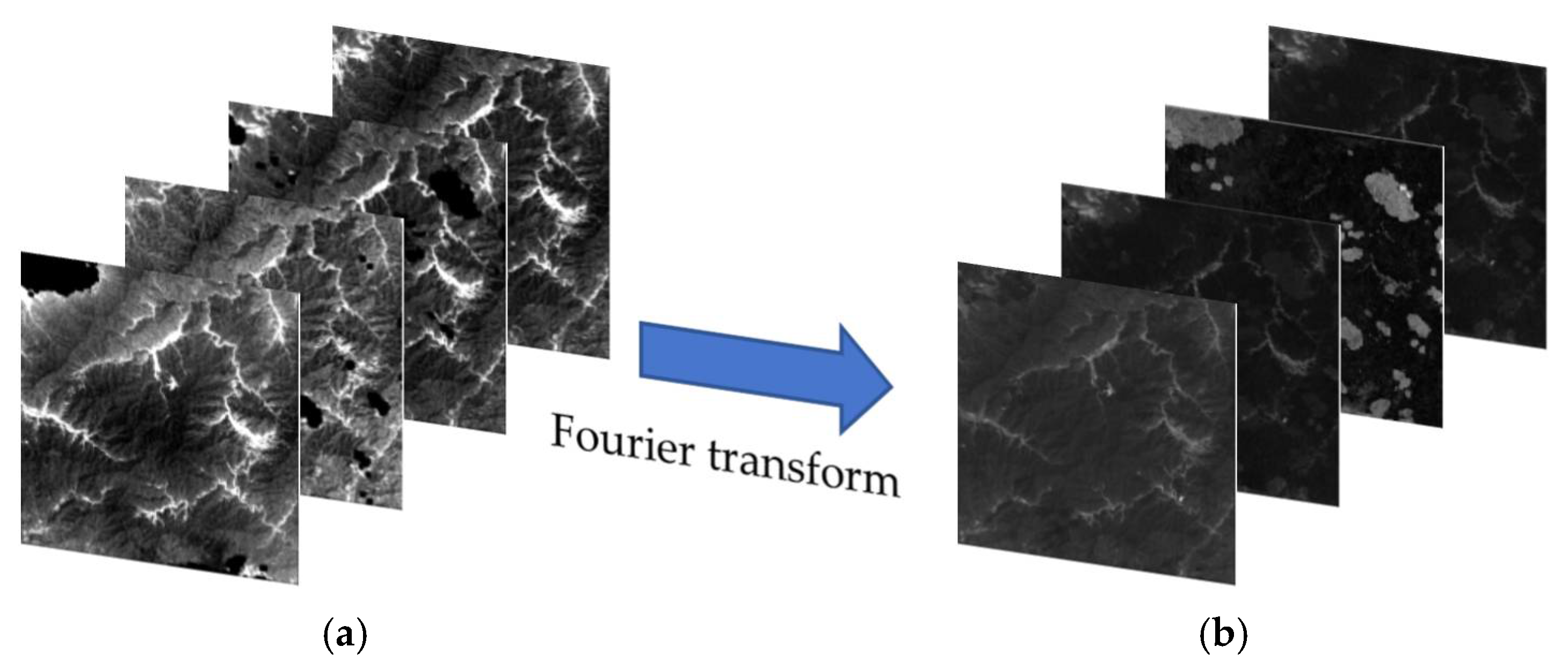
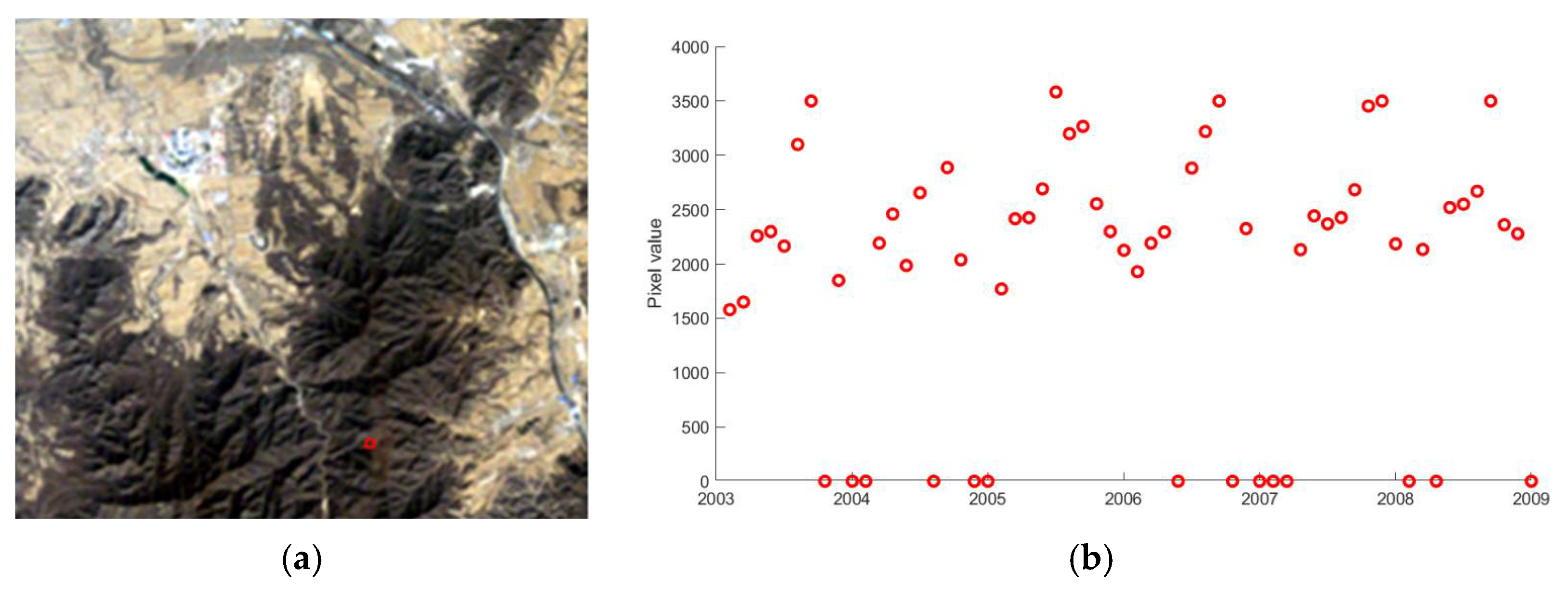
Examples of a rearranged spatial–temporal tensor and the spatial–frequential tensor are shown in Figure 2. The low-frequency part represents slowly changing or constant land features, shown in the first two images in Figure 2b, and the high-frequency part represents significantly changed land features, clouds and noise, as shown in the last two images in Figure 2b. Figure 3b shows the time-series scatter plot of the near-infrared band from 2003 to 2008 for one pixel of Figure 3a, where the value 0 represents contamination by clouds or data invalidation. After removing the influence of clouds, the periodicity of land features that changes with seasons can be seen in the long-term image sequences. Figure 4 shows the Fourier transform spectrum curve of Figure 3. The maximum value represents zero frequency. The two large values denoted by red dots in the low-frequency part are caused by the periodic variation of land features. Noise and clouds appear in the high-frequency part.
According to frequency spectrum characteristics of the spatial–frequential tensor, we proposed the following operations for X ^ . First, in order to maintain the low-frequency land features and weaken the high-frequency noise caused by clouds, a Gaussian low-pass filter is applied to X ^ in the frequency spectrum. Second, spatial adaptive weights determined by the frequency spectrum are performed to achieve the joint spatial–temporal low-rank constraint.
According to the properties of Fourier transform, there is a conjugate symmetry in the frequency domain of X ^ . The Gaussian filter is designed as follows:
f ( i ) = e ( i 1 ) 2 2 σ 2 ,
where i = 1 , , t + 1 2 , f ( i + 1 ) = f ( t i + 1 ) , and σ is a pre-set constant.
We define each spatial matrix of X ^ as X ^ i , i = 1 , , t . Due to X ^ i representing different frequency parts, when the same threshold is applied to perform the spatial low-rank processing of X ^ i , it will cause the loss of land feature information. In order to maintain land feature information in the image reconstruction, we choose the adaptive weight ω i for X ^ i according to the importance of the information from X ^ 1 to X ^ t .
X ^ i is defined as the normalized mean value k i as follows:
k i = m i i = 1 t m i ,
where m i denotes the mean value of X ^ i . A larger k i means more important information is contained in X ^ i , and a smaller ω i should be used in the low-rank processing. The adaptive weight ω i of each spatial matrix is defined as follows:
ω i = 1 k i 2 ρ i = 1 t 1 k i 2 .
where ρ is a pre-set constant.

2.3. Model Optimization

We define the augmented Lagrangian equation as follows:
L ρ ( M , X , B ) = M * + B , M X + ρ 2 M X F 2 .
where M , B and X are updated by the alternating direction method of multipliers (ADMM) [39]. M has a close-form solution:
M k + 1 = ifft ( D ω i ( f ( i ) fft ( X k + B k ρ ) ) ) .
where k is the iteration time. ifft ( ) is the Inverse Fast Fourier Transform. The adaptive weight ω i is determined by Equation (8). For X , it is updated as follows:
X k + 1 = { M k + 1 1 ρ B k   if   Ω i j k = 0 ; X ( 0 )                                     if   Ω i j k = 1 .
For B , it is updated as follows:
B k + 1 = B k ρ ( M k + 1 X k + 1 ) .
In this paper, the initial ρ is set to 10 4 . Later, to accelerate convergence, ρ will be iteratively increased by ρ k + 1 = t ρ k , t [ 1.1 , 1.2 ] . The solution process of FMTC is shown in Algorithm 1.
Algorithm 1 Optimization of the FMTC method
Input: Original remote sensing data Y , parameter ρ .
Initialize:  M 0 = B 0 = 0 ,   max   iteration   times   K = 200 .
for i = 0 to b do
    Obtain the rearranged spatial–temporal tensor X 0 for each band.
    for k = 0 to K do
        Update M by Equation (10);
        Update X by Equation (11);
        Update B by Equation (12);
    end for;
    repeat until convergence;
end for;
Output: Reconstructed image data X .

3. Experimental Results

3.1. Experimental Data

In this part, Landsat Collection 1 L1TP data from 2003 to 2018 in Beijing have been selected as the experiment data, as shown in Table 1. The experiment data include five simulated datasets and two real datasets based on different land-cover types and cloud areas, respectively. In order to demonstrate the effectiveness of FMTC, five algorithms are selected for comparison, including HaLRTC [27], AWTC [28], NL-LRTC [29], TVLRSD [30] and ST-Tensor [31].

3.2. Evaluation Indicators

In the simulated experiments, the Peak Signal-to-Noise Ratio (PSNR) [40], Structural Similarity (SSIM) [41] and Spectral Angle Mapper (SAM) [42] are chosen to evaluate the reconstructed images from the spatial and spectral perspectives.
The PSNR is calculated as follows:
PSNR = 10 log 10 ( M A X 2 MSE ) = 20 log 10 ( M A X MSE ) ;
MSE = 1 m n i = 0 m 1 j = 0 n 1 I ( i , j ) K ( i , j ) 2 .
where M A X is the maximum pixel value of the original image, and I ( i , j ) and K ( i , j ) denote the ( i , j ) th pixel values of the original image and the reconstructed image, respectively. m and n are the spatial sizes of those images.
The SSIM is calculated as follows:
SSIM ( x , y ) = ( 2 μ x μ y + c 1 ) ( 2 σ x y + c 2 ) ( μ x 2 + μ y 2 + c 1 ) ( σ x 2 + σ y 2 + c 2 ) .
where μ x and μ y represent the mean values of the original image and the reconstructed image, respectively. σ x and σ y represent the standard deviations. σ x y represents the covariance.
The SAM is calculated as follows:
SAM = arccos ( ( x 1 y 1 + + x n y n ) / ( x 1 2 + + x n 2 y 1 2 + + y n 2 ) ) .
where ( x 1 , , x n ) and ( y 1 , , y n ) denote the original image and reconstructed image of the spectral vectors.
In the real data experiments, the above evaluation indicators cannot be used because there was no reference image. Therefore, the information entropy (IE) [43] and the average gradient (AG) [44] are used to evaluate the reconstructed image. In addition, the effectiveness of the algorithm can be evaluated by the consistency of spatial images, the clarity of feature targets and the continuity of the time-series curve.
Information entropy of the reconstructed image is calculated as follows:
IE = t G p t log 2 p t .
where p t is the probability of value t . G is the maximum pixel value of the reconstructed image.
The average gradient of the reconstructed image is calculated as follows:
AG = 1 ( m 1 ) ( n 1 ) × i = 1 m 1 j = 1 n 1 ( K ( i , j ) K ( i + 1 , j ) ) 2 + ( K ( i , j ) K ( i , j + 1 ) ) 2 2 .

3.3. Simulated Data Experiments

In the simulated experiments, the effect of clouds is simulated by masking a random area on the cloud-free images. In order to demonstrate the effectiveness of FMTC on different land-cover types and missing areas, two simulated experiments were conducted. One is based on datasets 1–4 with four land-cover types, the other is based on dataset 5 with different sizes of missing areas. The information of the datasets is shown in Table 2.

3.3.1. The Experiment Based on Different Land-Cover Types

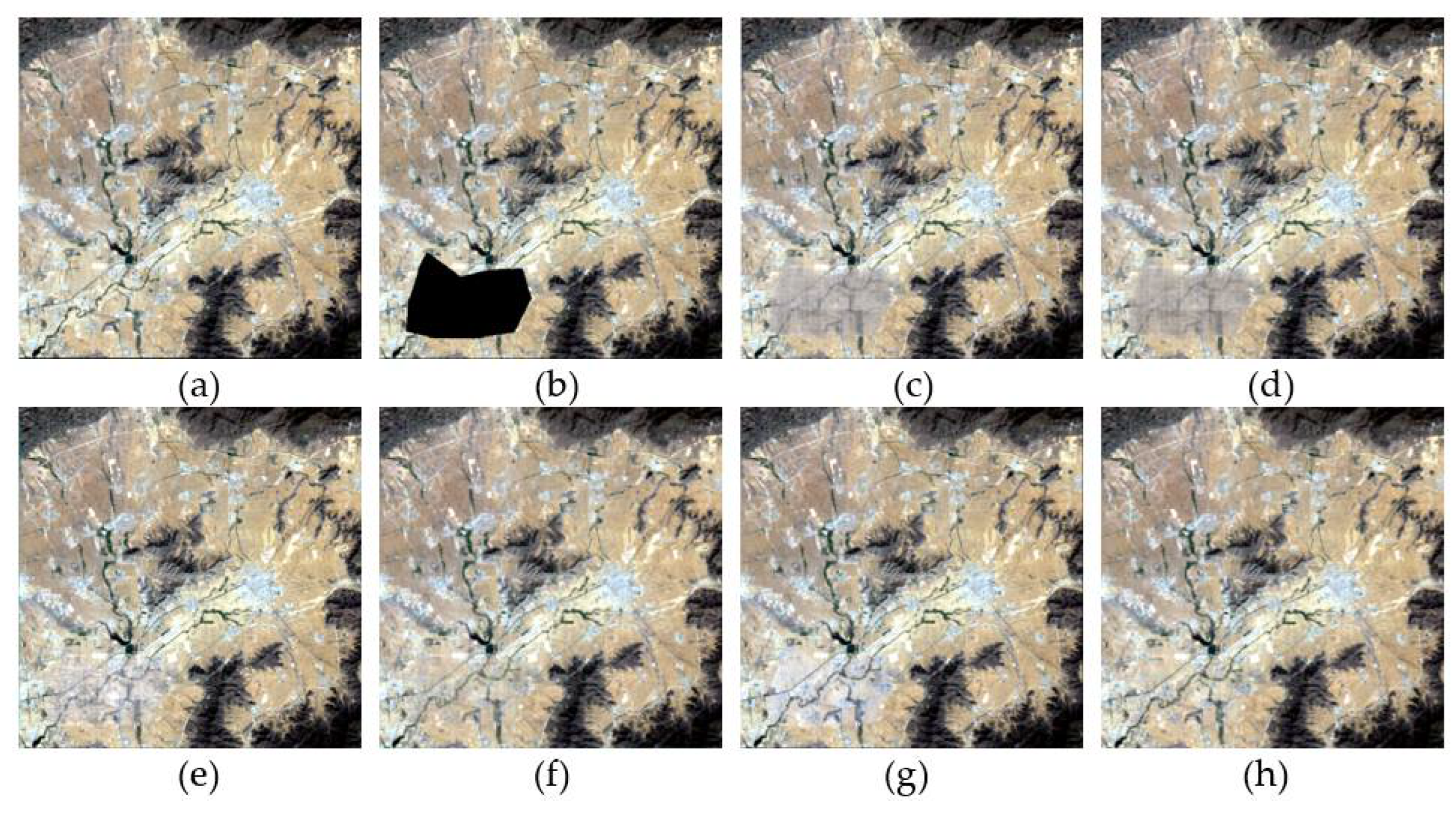
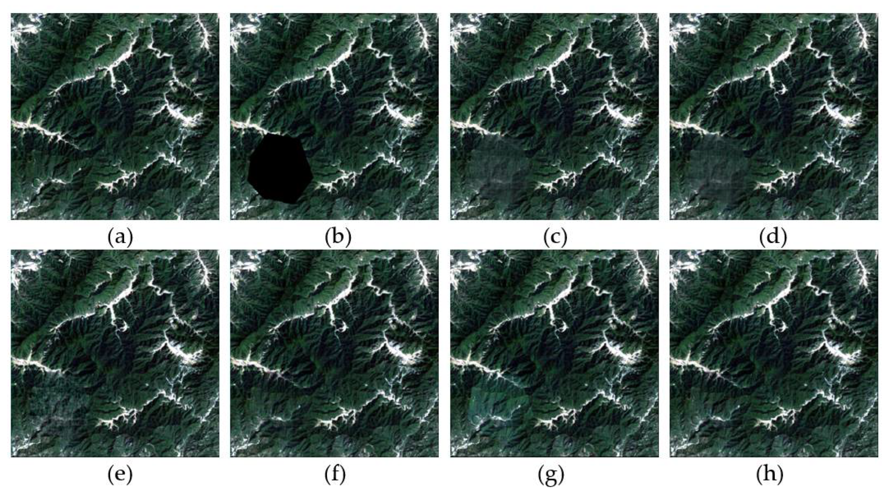
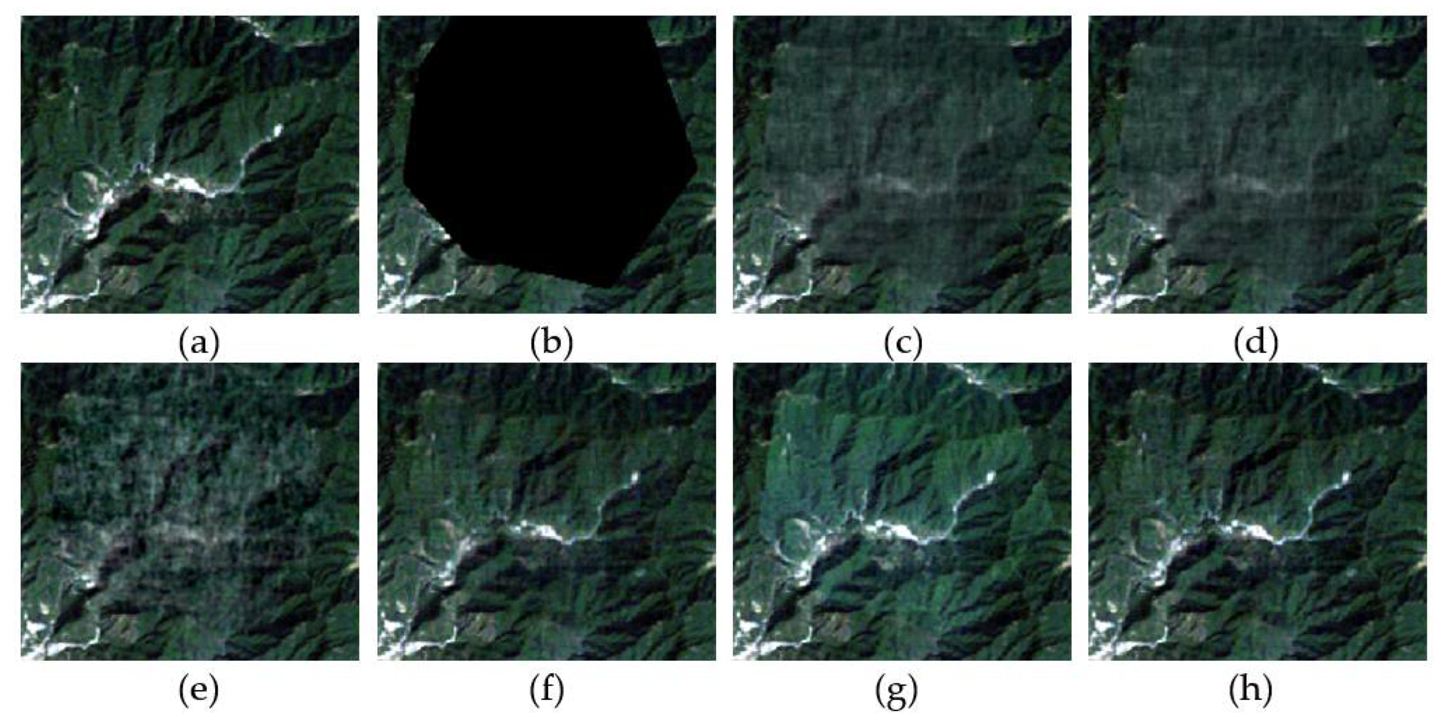
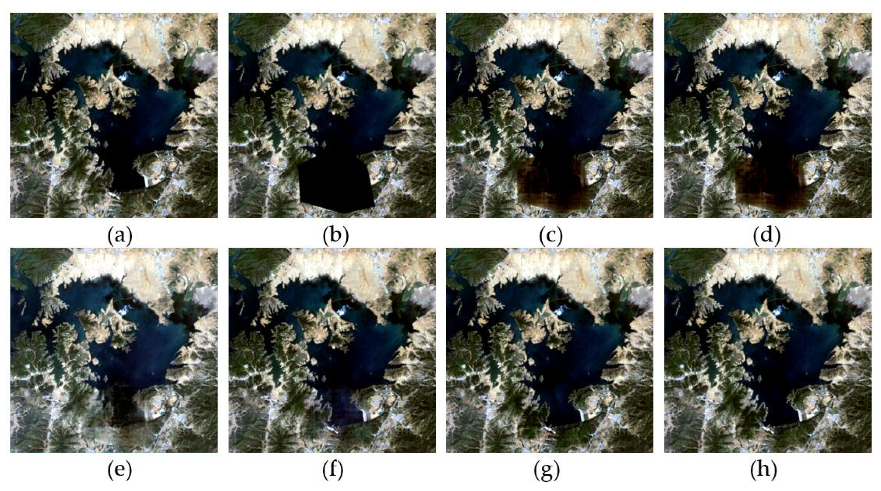
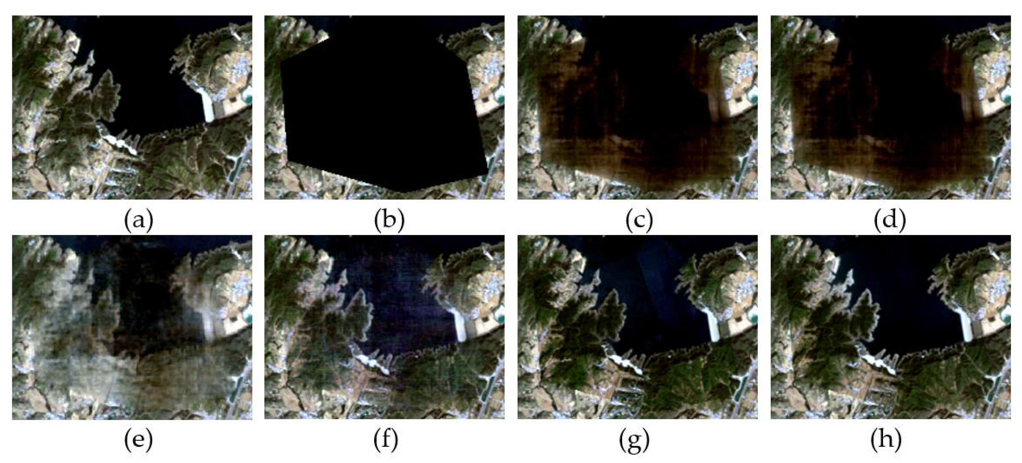
In this part, Landsat-5 datasets for four different regions in Beijing from 2003 to 2011 were selected, as shown in Table 2. The experiment results are shown in Figure 5, Figure 6, Figure 7, Figure 8, Figure 9, Figure 10, Figure 11 and Figure 12. Figure 5a, Figure 7a, Figure 9a and Figure 11a are true-color composition images (red—band 3, green—band 2, and blue—band 1). The simulated data have been generated from random missing areas where the pixel values were set to 0, as shown in Figure 5b, Figure 7b, Figure 9b and Figure 11b. Visual comparisons of FMTC with other algorithms are shown in Figure 5c–h, Figure 7c–h, Figure 9c–h and Figure 11c–h. Figure 6, Figure 8, Figure 10 and Figure 12 show enhanced details of the images.
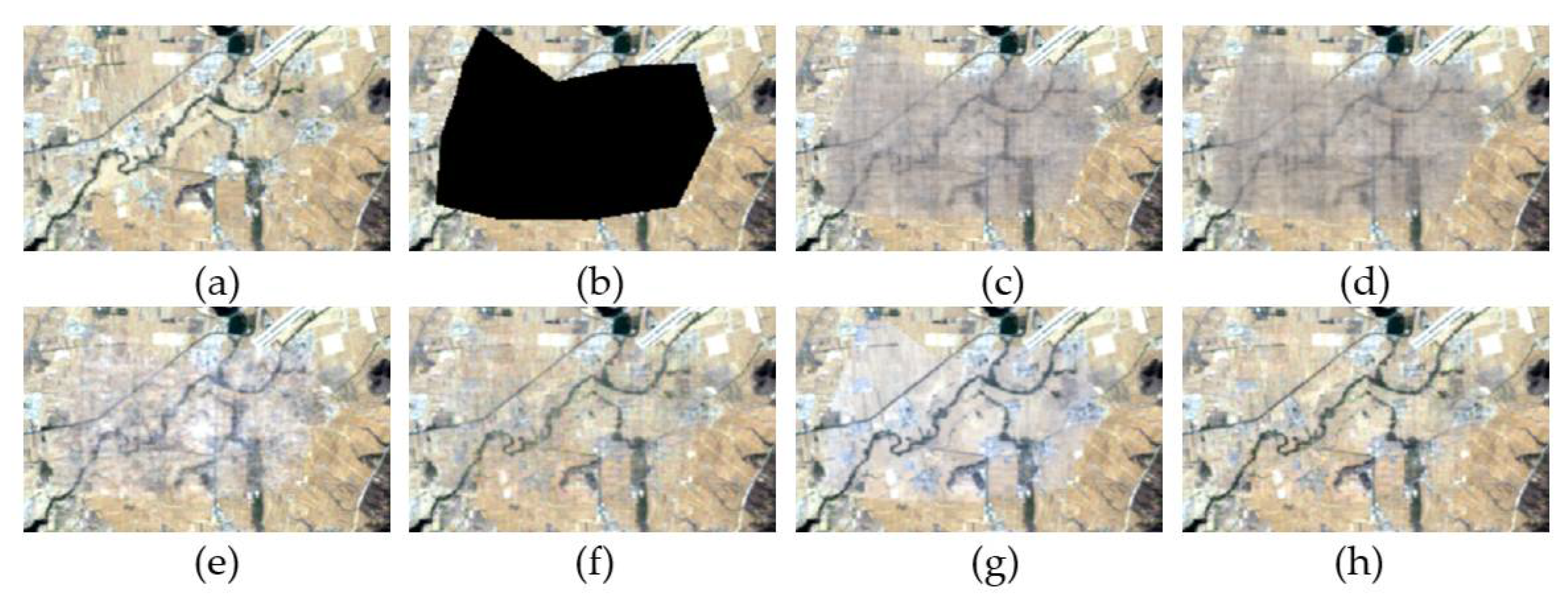
According to the enhanced detail shown in Figure 5, Figure 7, Figure 9 and Figure 11, we can see that the reconstructed results of HaLRTC and AWTC are blurry for four land-cover types because these algorithms only utilize the low-rank information derived from experimental data. The results of NL-LRTC are better than those of the first two algorithms, but still a bit fuzzy, which is due to the inappropriate choice of weights for the different modes of the tensor. TVLRSD can reconstruct the basic structure and details of the images, but the reconstructed details are still not clear. This may be because the matrix decomposition denoising the image and removing clouds makes images smooth and vague, but the details are not reconstructed. Although ST-Tensor maintains much of the detail of the images, the color of the reconstructed areas is inconsistent with that of the surroundings, due to the inappropriate choice of weights in the rearranged spatial–temporal tensor. In contrast, FMTC is able to ensure spatial detail as well as spectral consistency.
A quantitative comparison for the six algorithms applied to four land-cover types is shown in Table 3. HaLRTC, AWTC and NL-LRTC obtained poor results for all quantitative indicators. The results of TVLRSD and ST-Tensor are better than those of the above three algorithms. Generally speaking, FMTC can achieve much better results than the other five algorithms. Although the PSNR and SSIM of ST-Tensor seem to perform a little better than FMTC on impervious land, the SAM of ST-Tensor is significantly less effective than FMTC. In addition, FMTC shows outstanding performance on the three other land-cover types for each indicator. It can be seen that the results of the quantitative evaluation are consistent with visual examination. It is worth mentioning that FMTC is far less time-consuming than the other five algorithms.

3.3.2. The Experiment with Different Missing Sizes

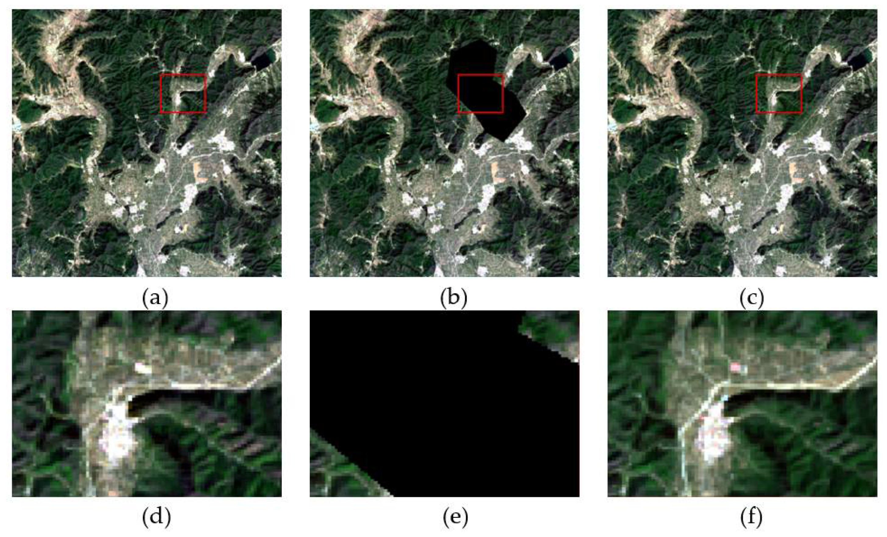
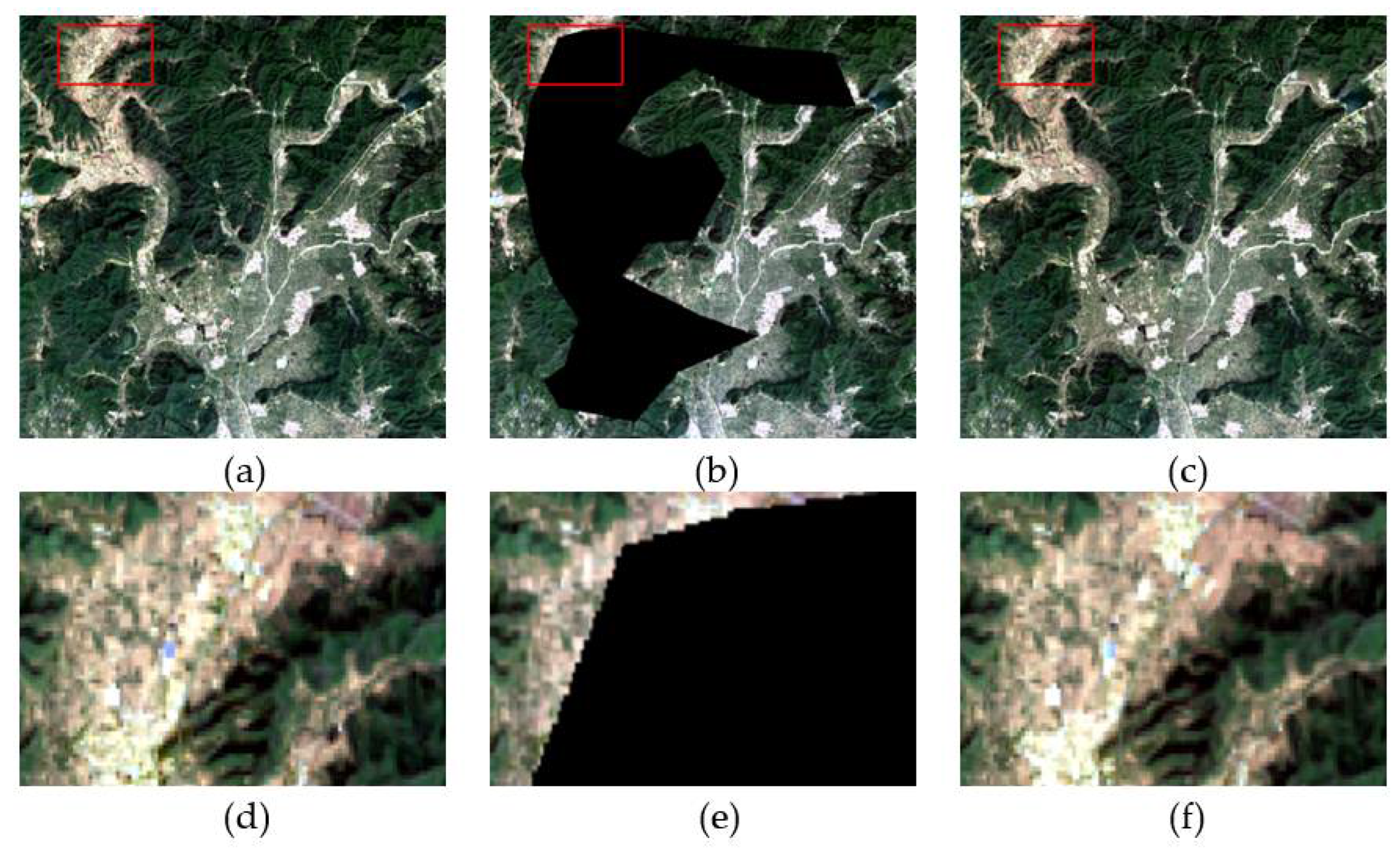
In this simulated experiment, dataset 5 was used to demonstrate the effectiveness of FMTC on different missing sizes. The proportions of the missing area are 6.01%, 19.26% and 32.48%, respectively. Figure 13, Figure 14 and Figure 15 are visual presentations of the results for three missing sizes, respectively. Figure 13a, Figure 14a and Figure 15a show true-color composition images (red—band 4, green—band 3, and blue—band 2). Simulated cloudy images are shown in Figure 13b, Figure 14b and Figure 15b. Figure 13c, Figure 14c and Figure 15c show the reconstructed images. Figure 13d–f, Figure 14d–f and Figure 15d–f show, in enhanced detail, the areas in the red boxes from Figure 13a–c, Figure 14a–c and Figure 15a–c, respectively.
Visually, the reconstructed results are consistent with the surroundings, and the proportion of the missing size reaches 32.48%. According to the areas with enhanced detail, the results of reconstruction approach the original images. In Figure 13d, a white road is depicted. In Figure 13f, the white road is reconstructed completely, owing to the time-series information utilized by FMTC. The above results demonstrate the effectiveness of using FMTC with different missing area sizes.
A quantitative comparison of the six algorithms with different missing sizes is shown in Table 4. As the proportion of missing size increases, the PSNR and SSIM of the first three algorithms decrease significantly, while the SAM increases. In contrast, the latter three algorithms are less sensitive to changes in missing sizes. Among all the algorithms, FMTC performs the best in most of the evaluation indicators. For different missing sizes, FMTC can obtain satisfactory results.

3.4. Real Data Experiments

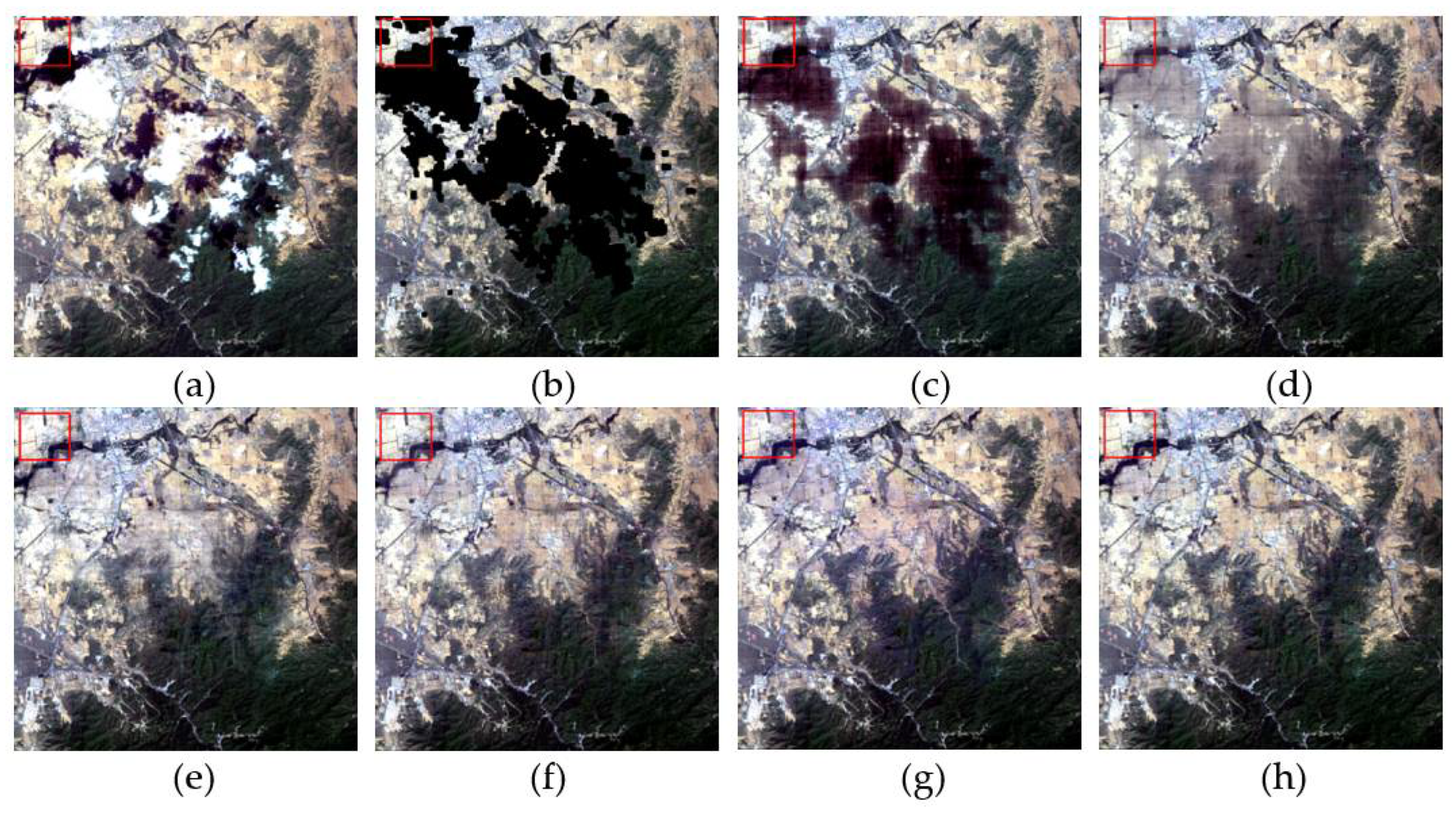
In experiments with real data, two datasets were selected, as shown in Table 5. For the real data, we used a Landsat quality assessment to mask clouds and cloud shadows. In order to demonstrate the effectiveness of applying FMTC on different data sources, two real data experiments were conducted.

3.4.1. Real Data Experiment 1

In this part, dataset 6 from Landsat-5 for the first real data experiment was selected. The main land cover type is impervious, and the others are vegetation and soil. Figure 16a shows the true-color composition image. Figure 16b shows the masked image. Visual comparisons of FMTC with other algorithms are shown in Figure 16c–h. Figure 17a–h show enhanced details of the areas in the red boxes.
The results of this experiment are similar to those of the simulated data experiment. The reconstructed results of HaLRTC and AWTC are not satisfactory and cannot meet the basic demands of reconstruction. The reconstructed details of TVLRSD and NL-LRTC are not clear, and the result of ST-Tensor is inconsistent with its surroundings. FMTC can not only clarify the reconstructed details, but it also ensures the consistency of the spectrum.
A quantitative comparison is shown in Table 6. The IE and AG of FMTC are better than those of other algorithms, indicating that the reconstructed details are richer and clearer. Figure 18 shows the time-series curves of six algorithms applied to one pixel from 2004 to 2006. The value 0 represents that the pixel was contaminated by cloud on that day. The curves of HaLRTC, AWTC and NL-LRTC display values of 0, leading to unsatisfactory results. The curves of TVLRSD and ST-Tensor are better than those of the first three algorithms, while they still show abrupt changes for the cloudy pixels. The curve of FMTC looks more continuous than those of all other algorithms. It can thus better characterize the temporal continuity and periodicity of land features.

3.4.2. Real Data Experiment 2

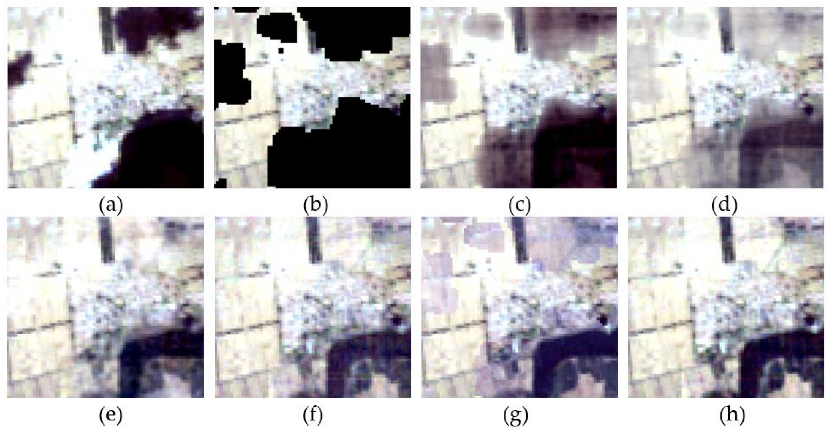
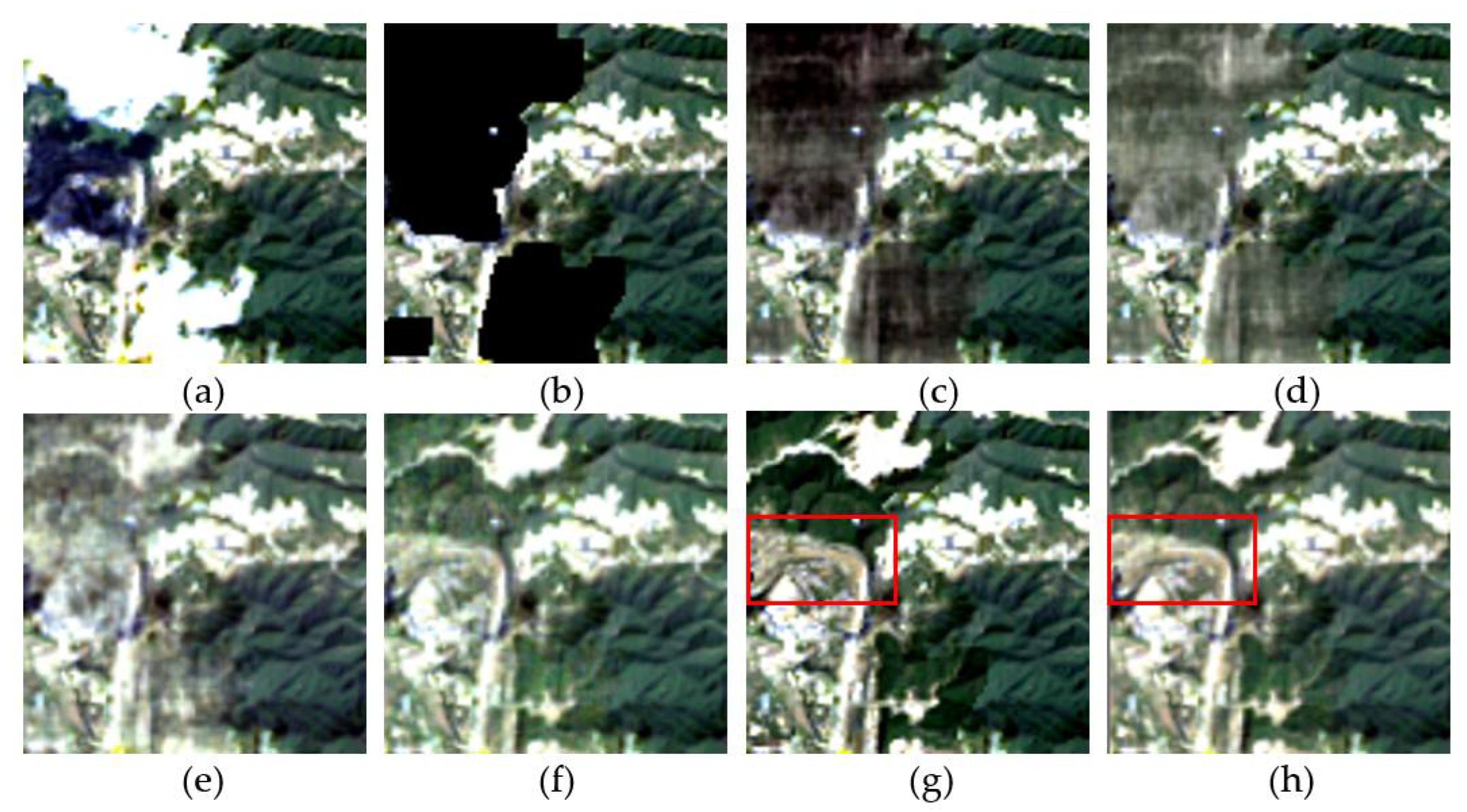
In this part, dataset 7 from Landsat-8 was selected for use in the second real data experiment. The main land cover type is vegetation, and the others are impervious and soil. Figure 19a is the original image. Figure 19b is the masked image. Visual comparisons of FMTC with other algorithms are shown in Figure 19c–h. Figure 20a–h show enhanced details of the areas in the red boxes.
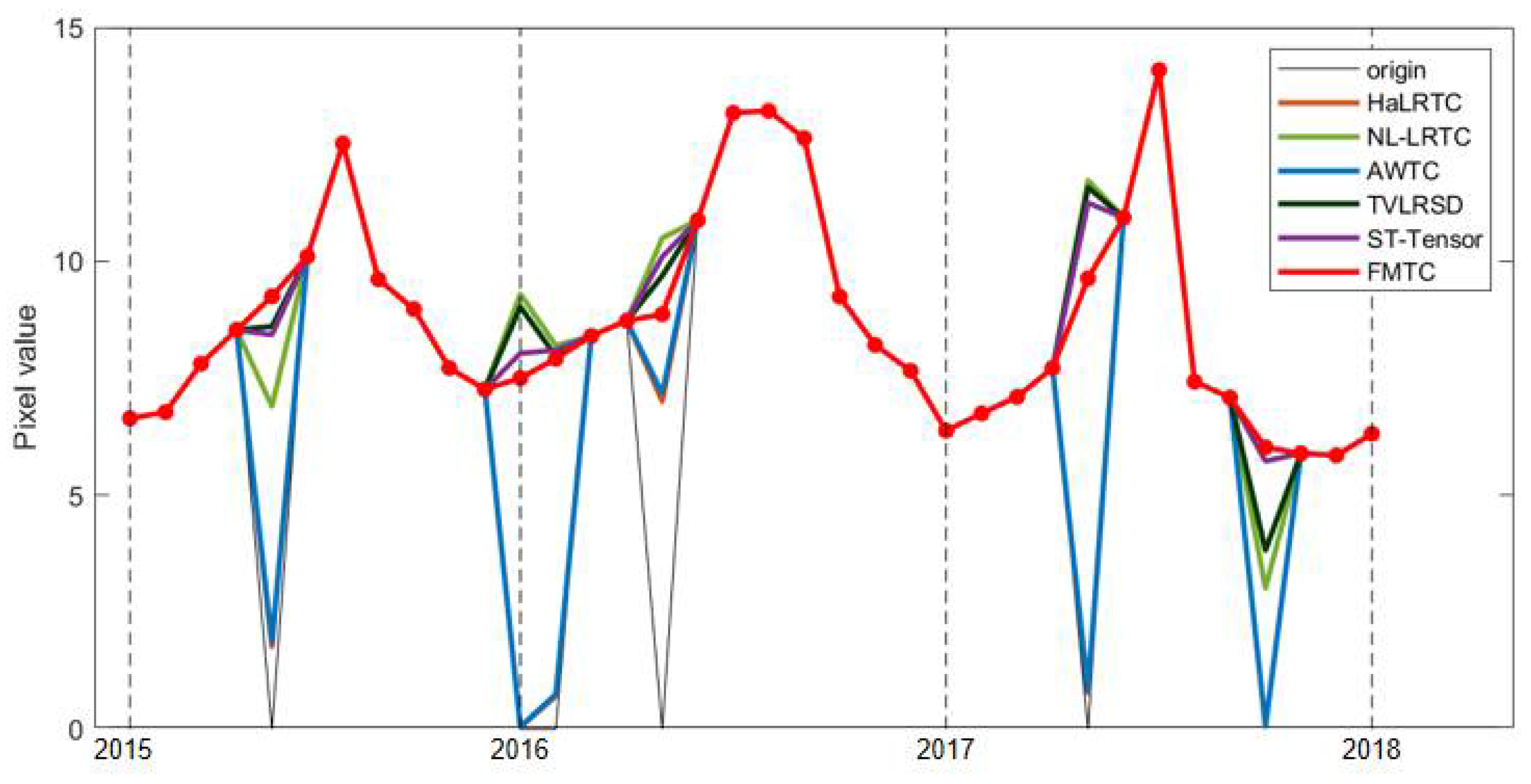
In terms of the visual effect, the results of this experiment are similar to those from real data experiment 1. As regards the areas of enhanced detail, TVLRSD is not clear enough. The white road, shown in the red box in Figure 20g,h, is not obvious in the reconstructed result of ST-Tensor, while the white road is reconstructed completely by FMTC. A quantitative evaluation is shown in Table 7. The time-series curves of the six algorithms applied to one pixel from 2015 to 2017 are shown in Figure 21. FMTC achieves the best performance, with excellent reconstructions from different data sources.

4. Conclusions

In this paper, we propose a frequency spectrum-modulated tensor completion method for multi-temporal remote sensing image inpainting. We rearrange the original four-dimensional tensor to establish a series of spatial–temporal tensors with low-rank properties. Fourier transform is introduced in the temporal dimension to generate the spatial–frequential tensor. The spatial adaptive weights are determined by the spectral properties of the time-domain signal, which is filtered using the Gaussian low-pass filtering to achieve joint spatial–temporal low-rank results. The experimental results based on both simulated and real datasets are presented to verify that FMTC can reconstruct missing data, starting from different land-cover types and different missing sizes. Compared with the other five methods used for the reconstruction of images, the results of FMTC are mostly better in terms of visual effects and quantitative evaluation. However, this method of image reconstruction still has some limitations. The reconstructed results may be affected by the detection of clouds and cloud shadows. In addition, FMTC encounters some limitations when applied to fickle objects, such as abrupt water.

Author Contributions

Conceptualization, H.T.; methodology, Z.C. and H.T.; resources, H.T. and L.J.; data curation, H.T. and L.J.; writing—original draft preparation, Z.C.; writing—review and editing, Z.C., H.T., P.Z., Y.Z., L.J. and X.X.; visualization, Z.C., H.T., P.Z., Y.Z. and L.J.; project administration, H.T.; funding acquisition, L.J. All authors have read and agreed to the published version of the manuscript.

Funding

This research was funded by the Second Tibetan Plateau Scientific Expedition and Research Program (grant number 2019QZKK0206), and the National Key Research and Development Program of China (grant number 31400).

Conflicts of Interest

The authors declare no conflict of interest.

References

  1. Leh, M.; Bajwa, S.; Chaubey, I. Impact of Land Use Change on Erosion Risk: An Integrated Remote Sensing, Geographic Information System and Modeling Methodology. Land Degrad. Dev. 2011, 24, 409–421. [Google Scholar] [CrossRef]
  2. Field, C.B.; Randerson, J.T.; Malmström, C.M. Global net primary production: Combining ecology and remote sensing. Remote Sens. Environ. 1995, 51, 74–88. [Google Scholar] [CrossRef] [Green Version]
  3. Shahzad, M.; Zhu, X.X. Automatic Detection and Reconstruction of 2-D/3-D Building Shapes from Spaceborne TomoSAR Point Clouds. IEEE Trans. Geosci. Remote Sens. 2016, 54, 1292–1310. [Google Scholar] [CrossRef] [Green Version]
  4. Nasrabadi, N.M. Hyperspectral Target Detection: An Overview of Current and Future Challenges. IEEE Signal Process. Mag. 2014, 31, 34–44. [Google Scholar] [CrossRef]
  5. Mou, L.; Ghamisi, P.; Zhu, X.X. Unsupervised Spectral–Spatial Feature Learning via Deep Residual Conv–Deconv Network for Hyperspectral Image Classification. IEEE Trans. Geosci. Remote Sens. 2017, 56, 391–406. [Google Scholar] [CrossRef] [Green Version]
  6. Tarabalka, Y.; Fauvel, M.; Chanussot, J.; Benediktsson, J.A. SVM- and MRF-Based Method for Accurate Classification of Hyperspectral Images. IEEE Geosci. Remote Sens. Lett. 2010, 7, 736–740. [Google Scholar] [CrossRef] [Green Version]
  7. Li, S.; Yin, H.; Fang, L. Remote Sensing Image Fusion via Sparse Representations Over Learned Dictionaries. IEEE Trans. Geosci. Remote Sens. 2013, 51, 4779–4789. [Google Scholar] [CrossRef]
  8. Xie, D.; Gao, F.; Sun, L.; Anderson, M. Improving Spatial–temporal Data Fusion by Choosing Optimal Input Image Pairs. Remote Sens. 2018, 10, 1142. [Google Scholar] [CrossRef] [Green Version]
  9. Shen, H.; Li, X.; Cheng, Q.; Zeng, C.; Yang, G.; Li, H.; Zhang, L. Missing Information Reconstruction of Remote Sensing Data: A Technical Review. IEEE Geosci. Remote Sens. Mag. 2015, 3, 61–85. [Google Scholar] [CrossRef]
  10. Siu, W.C.; Hung, K.W. Review of image interpolation and super-resolution. In Proceedings of the Signal & Information Processing Association Summit & Conference, Hollywood, CA, USA, 3–6 December 2012. [Google Scholar]
  11. Chao, Y.; Chen, L.; Lin, S.; Meng, F.; Li, S. Kriging interpolation method and its application in retrieval of MODIS aerosol optical depth. In Proceedings of the International Conference on Geoinformatics, Shanghai, China, 24–26 June 2011; pp. 1–6. [Google Scholar]
  12. Lorenz, L.; Melgant, F.; Merrier, G. Multiresolution inpainting for reconstruction of missing data in VHR images. In Proceedings of the 2011 IEEE International Geoscience and Remote Sensing Symposium, Vancouver, BC, Canada, 24–29 July 2011. [Google Scholar]
  13. Kitchener, M.A.; Bouzerdoum, A.; Phung, S.L. A Compressive Sensing Approach to Image Restoration. In Proceedings of the 2010 International Conference on Digital Image Computing: Techniques and Applications, Sydney, Australia, 1–3 December 2010; pp. 111–115. [Google Scholar]
  14. Zhang, J.; Zhao, D.; Gao, W. Group-based sparse representation for image restoration. IEEE Trans. Image Process. 2014, 23, 3336–3351. [Google Scholar] [CrossRef] [Green Version]
  15. Shen, H.; Zhang, L. A MAP-Based Algorithm for Destriping and Inpainting of Remotely Sensed Images. IEEE Trans. Geosci. Remote Sens. 2009, 47, 1492–1502. [Google Scholar] [CrossRef]
  16. Cheng, Q.; Shen, H.; Zhang, L.; Li, P. Inpainting for Remotely Sensed Images with a Multichannel Nonlocal Total Variation Model. IEEE Trans. Geosci. Remote Sens. 2014, 52, 175–187. [Google Scholar] [CrossRef]
  17. Rakwatin, P.; Takeuchi, W.; Yasuoka, Y. Restoration of Aqua MODIS Band 6 Using Histogram Matching and Local Least Squares Fitting. IEEE Trans. Geosci. Remote Sens. 2009, 47, 613–627. [Google Scholar] [CrossRef]
  18. Roy, D.P.; Ju, J.; Lewis, P.; Schaaf, C.; Gao, F.; Hansen, M.; Lindquist, E. Multi-temporal MODIS–Landsat data fusion for relative radiometric normalization, gap filling, and prediction of Landsat data. Remote Sens. Environ. 2008, 112, 3112–3130. [Google Scholar] [CrossRef]
  19. Zhang, L.; Wang, Z.; Zhang, J.; Jin, J.; Liang, J.; Liao, M.; Yan, K.; Peng, Q. A new cloud removal algorithm for multi-spectral images. In Proceedings of the MIPPR 2005: SAR and Multispectral Image Processing, Wuhan, China, 31 October–2 November 2005. [Google Scholar]
  20. Feng, C.; Ma, J.W.; Dai, Q.; Chen, X. An improved method for cloud removal in ASTER data change detection. In Proceedings of the IEEE International Geoscience & Remote Sensing Symposium, Anchorage, AK, USA, 20–24 September 2004. [Google Scholar]
  21. Zhang, Y.; Guindon, B.; Cihlar, J. An image transform to characterize and compensate for spatial variations in thin cloud contamination of Landsat images. Remote Sens. Environ. 2002, 82, 173–187. [Google Scholar] [CrossRef]
  22. Wang, Y.; Jiao, Q.; Li, J.; Luo, W.; Liu, X.; Lei, B.; Yang, J.; Zhang, B. Information reconstruction in the cloud removing area based on multi-temporal CHRIS images. In Proceedings of the MIPPR 2007: Remote Sensing and GIS Data Processing and Applications; and Innovative Multispectral Technology and Applications, Wuhan, China, 15–17 November 2007. [Google Scholar]
  23. Melgani, F. Contextual reconstruction of cloud-contaminated multitemporal multispectral images. IEEE Trans. Geosci. Remote Sens. 2006, 44, 442–455. [Google Scholar] [CrossRef]
  24. Zhang, X.; Qin, F.; Qin, Y. Study on the Thick Cloud Removal Method Based on Multi-Temporal Remote Sensing Images. In Proceedings of the 2010 International Conference on Multimedia Technology, Ningbo, China, 29–31 October 2010. [Google Scholar]
  25. Lin, C.-H.; Tsai, P.-H.; Lai, K.-H.; Chen, J.-Y. Cloud Removal from Multitemporal Satellite Images Using Information Cloning. IEEE Trans. Geosci. Remote Sens. 2013, 51, 232–241. [Google Scholar] [CrossRef]
  26. Li, X.; Shen, H.; Zhang, L.; Zhang, H.; Yuan, Q.; Yang, G. Recovering Quantitative Remote Sensing Products Contaminated by Thick Clouds and Shadows Using Multitemporal Dictionary Learning. IEEE Trans. Geosci. Remote Sens. 2014, 52, 7086–7098. [Google Scholar]
  27. Liu, J.; Musialski, P.; Wonka, P.; Ye, J. Tensor completion for estimating missing values in visual data. IEEE Trans. Pattern Anal. Mach. Intell. 2013, 35, 208–220. [Google Scholar] [CrossRef] [PubMed]
  28. Ng, M.K.-P.; Yuan, Q.; Yan, L.; Sun, J. An Adaptive Weighted Tensor Completion Method for the Recovery of Remote Sensing Images with Missing Data. IEEE Trans. Geosci. Remote Sens. 2017, 55, 3367–3381. [Google Scholar] [CrossRef]
  29. Ji, T.Y.; Yokoya, N.; Zhu, X.X.; Huang, T.Z. Nonlocal tensor completion for multitemporal remotely sensed images’ inpainting. IEEE Trans. Geosci. Remote Sens. 2018, 56, 3047–3061. [Google Scholar] [CrossRef]
  30. Chen, Y.; He, W.; Yokoya, N.; Huang, T.-Z. Blind cloud and cloud shadow removal of multitemporal images based on total variation regularized low-rank sparsity decomposition. ISPRS J. Photogramm. Remote Sens. 2019, 157, 93–107. [Google Scholar] [CrossRef]
  31. Chu, D.; Shen, H.; Guan, X.; Chen, J.M.; Li, X.; Li, J.; Zhang, L. Long time-series NDVI reconstruction in cloud-prone regions via spatial–temporal tensor completion. Remote Sens. Environ. 2021, 264, 112632. [Google Scholar] [CrossRef]
  32. Duan, C.; Pan, J.; Li, R. Thick Cloud Removal of Remote Sensing Images Using Temporal Smoothness and Sparsity Regularized Tensor Optimization. Remote Sens. 2020, 12, 3446. [Google Scholar] [CrossRef]
  33. Lin, J.; Huang, T.-Z.; Zhao, X.-L.; Chen, Y.; Zhang, Q.; Yuan, Q. Robust Thick Cloud Removal for Multitemporal Remote Sensing Images Using Coupled Tensor Factorization. IEEE Trans. Geosci. Remote Sens. 2022, 60, 1–16. [Google Scholar] [CrossRef]
  34. Liu, N.; Li, W.; Wang, Y.; Tao, R.; Du, Q.; Chanussot, J. A Survey on Hyperspectral Image Restoration: From the View of Low-Rank Tensor Approximation. arXiv 2022, arXiv:2205.08839. [Google Scholar]
  35. Liu, N.; Li, W.; Tao, R.; Du, Q.; Chanussot, J. Multigraph-Based Low-Rank Tensor Approximation for Hyperspectral Image Restoration. IEEE Trans. Geosci. Remote Sens. 2022, 60, 1–14. [Google Scholar] [CrossRef]
  36. Kurucz, M.; Benczúr, A.; Csalogány, K. Methods for large scale SVD with missing values. In Proceedings of the KDD Cup and Workshop, San Jose, CA, USA, 12 August 2007. [Google Scholar]
  37. Cai, J.-F.; Candès, E.J.; Shen, Z. A Singular Value Thresholding Algorithm for Matrix Completion. SIAM J. Optim. 2010, 20, 1956–1982. [Google Scholar] [CrossRef]
  38. Lu, C.; Feng, J.; Chen, Y.; Liu, W.; Lin, Z.; Yan, S. Tensor Robust Principal Component Analysis with a New Tensor Nuclear Norm. IEEE Trans. Pattern Anal. Mach. Intell. 2020, 42, 925–938. [Google Scholar] [CrossRef] [Green Version]
  39. Lin, Z.; Chen, M.; Ma, Y. The Augmented Lagrange Multiplier Method for Exact Recovery of Corrupted Low-Rank Matrices. arXiv 2010, arXiv:1009.5055. [Google Scholar]
  40. Shen, H.; Li, X.; Zhang, L.; Tao, D.; Zeng, C. Compressed Sensing-Based Inpainting of Aqua Moderate Resolution Imaging Spectroradiometer Band 6 Using Adaptive Spectrum-Weighted Sparse Bayesian Dictionary Learning. IEEE Trans. Geosci. Remote Sens. 2014, 52, 894–906. [Google Scholar] [CrossRef]
  41. Wang, Z.; Bovik, A.C.; Sheikh, H.R.; Simoncelli, E.P. Image quality assessment: From error visibility to structural similarity. IEEE Trans. Image Process. 2004, 13, 600–612. [Google Scholar] [CrossRef] [PubMed] [Green Version]
  42. Kruse, F.A.; Lefkoff, A.B.; Boardman, J.W.; Heidebrecht, K.B.; Shapiro, A.T.; Barloon, P.J.; Goetz, A.F.H. The spectral image processing system (SIPS)-interactive visualization and analysis of imaging spectrometer data. Remote Sens. Environ. 1993, 44, 145–163. [Google Scholar] [CrossRef]
  43. Ferraro, M.; Boccignone, G.; Caelli, T. Entropy-based representation of image information. Pattern Recognit. Lett. 2002, 23, 1391–1398. [Google Scholar] [CrossRef]
  44. Li, Z.; Jing, Z.; Yang, X.; Sun, S. Color transfer based remote sensing image fusion using non-separable wavelet box transform. Pattern Recognit. Lett. 2005, 26, 2006–2014. [Google Scholar] [CrossRef]
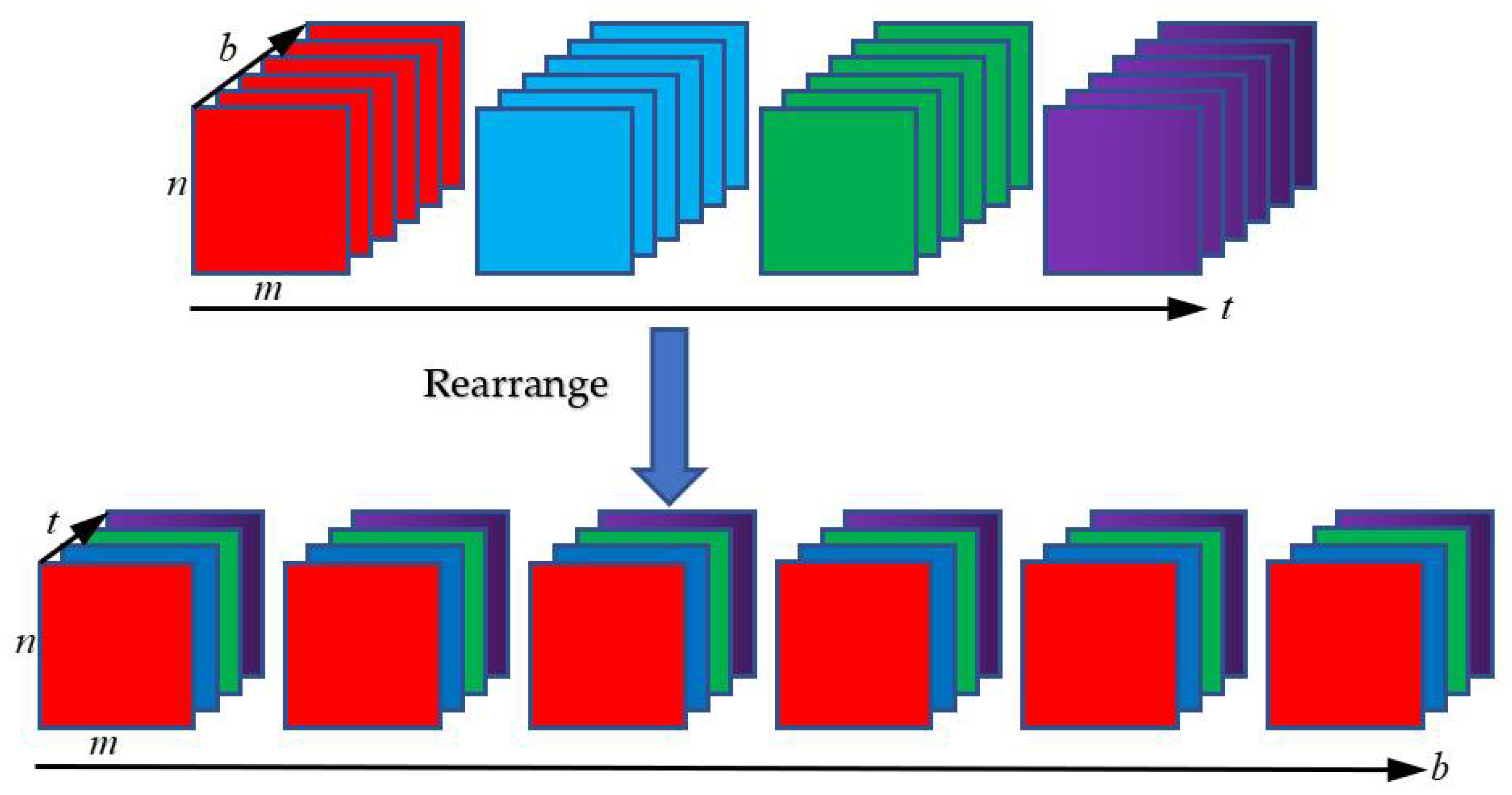
Figure 1. Multi-temporal remote sensing images rearrangement.
Remotesensing 15 01230 g001
Figure 2. (a) The rearranged spatial–temporal tensor; (b) the spatial–frequential tensor.
Remotesensing 15 01230 g002
Figure 3. (a) Original image (20030327). (b) Scatter plot of the time series of the near-infrared band from 2003 to 2008 for a pixel of (a) in the red box.
Remotesensing 15 01230 g003
Figure 4. The frequency spectrum curve of the above data in Figure 3.
Remotesensing 15 01230 g004
Figure 5. The simulated experiment performed on dataset 1: (a) original image; (b) simulated cloudy image; (ch) reconstructed images with HaLRTC, AWTC, NL-LRTC, TVLRSD, ST-Tensor and FMTC algorithms, respectively.
Remotesensing 15 01230 g005
Figure 6. Enhanced details from Figure 5a–h: (a) original image; (b) simulated cloudy image; (ch) reconstructed images of HaLRTC, AWTC, NL-LRTC, TVLRSD, ST-Tensor and FMTC algorithms, respectively.
Remotesensing 15 01230 g006
Figure 7. The simulated experiment performed on dataset 2: (a) original image; (b) simulated cloudy image; (ch) reconstructed images with HaLRTC, AWTC, NL-LRTC, TVLRSD, ST-Tensor and FMTC algorithms, respectively.
Remotesensing 15 01230 g007
Figure 8. Enhanced details from Figure 7a–h: (a) original image; (b) simulated cloudy image; (ch) reconstructed images of HaLRTC, AWTC, NL-LRTC, TVLRSD, ST-Tensor and FMTC algorithms, respectively.
Remotesensing 15 01230 g008
Figure 9. The simulated experiment performed on dataset 3: (a) original image; (b) simulated cloudy image; (ch) reconstructed images of HaLRTC, AWTC, NL-LRTC, TVLRSD, ST-Tensor and FMTC algorithms, respectively.
Remotesensing 15 01230 g009
Figure 10. Enhanced details from Figure 9a–h: (a) original image; (b) simulated cloudy image; (ch) reconstructed images of HaLRTC, AWTC, NL-LRTC, TVLRSD, ST-Tensor and FMTC algorithms, respectively.
Remotesensing 15 01230 g010
Figure 11. The simulated experiment performed on dataset 4: (a) original image; (b) simulated cloudy image, (ch) reconstructed images of HaLRTC, AWTC, NL-LRTC, TVLRSD, ST-Tensor and FMTC algorithms, respectively.
Remotesensing 15 01230 g011
Figure 12. Enhanced details from Figure 11a–h: (a) original image; (b) simulated cloudy image; (ch) reconstructed images of HaLRTC, AWTC, NL-LRTC, TVLRSD, ST-Tensor and FMTC algorithms, respectively.
Remotesensing 15 01230 g012
Figure 13. The simulated experiment with a missing area of 6.01%: (a) original image; (b) simulated cloudy image; (c) reconstructed image; (df) enhanced details from red boxes in (ac).
Remotesensing 15 01230 g013
Figure 14. The simulated experiment with missing area of 19.26%: (a) original image; (b) simulated cloudy image; (c) reconstructed image; (df) enhanced details from red boxes in (ac).
Remotesensing 15 01230 g014
Figure 15. The simulated experiment with missing area of 32.48%: (a) original image; (b) simulated cloudy image; (c) reconstructed image; (df) enhanced details from red boxes in (ac).
Remotesensing 15 01230 g015
Figure 16. The real data experiment performed on dataset 6: (a) original image; (b) masked image; (ch) reconstructed images for HaLRTC, AWTC, NL-LRTC, TVLRSD, ST-Tensor and FMTC algorithms, respectively.
Remotesensing 15 01230 g016
Figure 17. Enhanced details from Figure 16a–h: (a) original image; (b) masked image (ch) reconstructed images of HaLRTC, AWTC, NL-LRTC, TVLRSD, ST-Tensor and FMTC algorithms, respectively.
Remotesensing 15 01230 g017
Figure 18. The time-series curves of six algorithms applied to one pixel from 2004 to 2006.
Remotesensing 15 01230 g018
Figure 19. The real data experiment performed on dataset 7: (a) original image; (b) masked image; (ch) reconstructed images for HaLRTC, AWTC, NL-LRTC, TVLRSD, ST-Tensor and FMTC algorithms, respectively.
Remotesensing 15 01230 g019
Figure 20. Enhanced detail from Figure 19a–h: (a) original image; (b) masked image; (ch) reconstructed images with HaLRTC, AWTC, NL-LRTC, TVLRSD, ST-Tensor and FMTC algorithms, respectively.
Remotesensing 15 01230 g020
Figure 21. The time-series curves of six algorithms applied to one pixel from 2015 to 2017.
Remotesensing 15 01230 g021
Table 1. Experiment data information.
SourceDurationResolutionBandSize
Landsat-52003–201130 m1–6 500 × 500
Landsat-82013–201830 m1–7 500 × 500
Table 2. Information on five datasets.
DatasetLocationLand-Cover TypesMask DateSource
Dataset 1Beijing City CenterImpervious17 May 2009Landsat-5
Dataset 2Yanqing, BeijingSoil26 April 2007Landsat-5
Dataset 3Huairou, BeijingVegetation2 June 2009Landsat-5
Dataset 4Miyun, BeijingWater7 May 2011Landsat-5
Dataset 5Pinggu, BeijingVegetation/Soil/Impervious18 May 2015Landsat-8
Table 3. Quantitative comparison of six algorithms applied to four land-cover types.
Land-Cover TypeIndicatorHaLRTCAWTCNL-LRTCTVLRSDST-TensorFMTC
ImperviousPSNR51.02451.95452.32553.49055.20155.021
SSIM0.99260.99350.99410.99580.99920.9990
SAM0.07670.07820.69890.06030.05330.0530
Time(s)161.59426.37649.48592.94839.64269.19
SoilPSNR38.83939.23540.86541.87641.91441.975
SSIM0.99410.99510.99710.99830.99840.9987
SAM0.04370.04210.03260.02950.02890.0271
Time(s)186.13438.46659.46526.35837.09294.14
VegetationPSNR38.68139.02440.21643.45343.47743.492
SSIM0.99850.99920.99930.99950.99960.9997
Time(s)168.38362.470.0457461.96710.46352.98
SAM0.05910.0588574.180.03760.03740.0358
WaterPSNR32.07632.70538.78341.68442.92643.003
SSIM0.96640.96960.97620.98260.98740.9901
SAM0.04020.013860.03640.03580.03270.0321
Time(s)390.34822.65776.04768.35910.67431.76
Table 4. Quantitative comparison of six algorithms with different missing sizes.
Missing SizeIndicatorHaLRTCAWTCNL-LRTCTVLRSDST-TensorFMTC
6.01%PSNR39.65840.67545.31948.35549.52149.531
SSIM0.99270.99410.99730.99840.99990.9998
SAM0.08630.08520.71260.06640.06350.0625
Time(s)191.19483.61593.45563.95784.55277.23
19.26%PSNR26.20826.78337.63443.63944.02244.083
SSIM0.92400.93360.97360.99590.99800.9979
SAM0.09240.09110.60890.04770.04460.0440
Time(s)326.74684.39715.64706.97936.21386.42
32.48%PSNR25.78526.19937.59940.86842.81542.844
SSIM0.83430.84820.91570.99450.99620.9964
SAM0.10180.09930.69430.04010.03740.0366
Time(s)403.51704.62903.49873.561017.55464.57
Table 5. Real data experiments’ datasets.
DatasetLocationDurationMask DateSourceLand Cover Type
Dataset 6Changpin, Beijing2003–201122 May 2005Landsat-5impervious/vegetation/soil
Dataset 7Mentougou, Beijing2013–201821 April 2017Landsat-8vegetation/impervious/soil
Table 6. Quantitative comparison of six algorithms applied to dataset 6.
IndicatorHaLRTCAWTCNL-LRTCTVLRSDST-TensorFMTC
IE6.86696.87566.93176.96536.94706.9955
AG0.04250.04380.04650.04690.04640.0476
Table 7. Quantitative comparisons of six algorithms applied to dataset 7.
IndicatorHaLRTCAWTCNL-LRTCTVLRSDST-TensorFMTC
IE6.68716.68716.68816.68996.69106.6913
AG0.03010.03120.03250.03360.03410.0341
Disclaimer/Publisher’s Note: The statements, opinions and data contained in all publications are solely those of the individual author(s) and contributor(s) and not of MDPI and/or the editor(s). MDPI and/or the editor(s) disclaim responsibility for any injury to people or property resulting from any ideas, methods, instructions or products referred to in the content.