Automated Identification of Thermokarst Lakes Using Machine Learning in the Ice-Rich Permafrost Landscape of Central Yakutia (Eastern Siberia)

Abstract

The current rate and magnitude of temperature rise in the Arctic are disproportionately high compared to global averages. Along with other natural and anthropogenic disturbances, this warming has caused widespread permafrost degradation and soil subsidence, resulting in the formation of thermokarst (thaw) lakes in areas of ice-rich permafrost. These lakes are hotspots of greenhouse gas emissions (CO₂ and CH₄), but with substantial spatial and temporal heterogeneity across Arctic and sub-Arctic regions. In Central Yakutia (Eastern Siberia, Russia), nearly half of the landscape has been affected by thermokarst processes since the early Holocene, resulting in the formation of more than 10,000 partly drained lake depressions (alas lakes). It is not yet clear how recent changes in temperature and precipitation will affect existing lakes and the formation of new thermokarst lakes. A multi-decadal remote sensing analysis of lake formation and development was conducted for two large study areas (~1200 km² each) in Central Yakutia. Mask Region-Based Convolutional Neural Networks (R-CNN) instance segmentation was used to semi-automate lake detection in Satellite pour l’Observation de la Terre (SPOT) and declassified US military (CORONA) images (1967–2019). Using these techniques, we quantified changes in lake surface area for three different lake types (unconnected alas lake, connected alas lake, and recent thermokarst lake) since the 1960s. Our results indicate that unconnected alas lakes are the dominant lake type, both in the number of lakes and total surface area coverage. Unconnected alas lakes appear to be more susceptible to changes in precipitation compared to the other two lake types. The majority of recent thermokarst lakes form within 1 km of observable human disturbance and their surface area is directly related to air temperature increases. These results suggest that climate change and human disturbances are having a strong impact on the landscape and hydrology of Central Yakutia. This will likely affect regional and global carbon cycles, with implications for positive feedback scenarios in a continued climate warming situation.

1. Introduction

Permafrost landscapes cover 20 million km² of the northern hemisphere and are particularly abundant in Siberia, Alaska, and northern Canada [1,2]. Regional and local hydrological and geological factors influence its spatial distribution, thickness, and ground ice content [3]. An important feature of permafrost is its storage of enough organic carbon (OC) to significantly impact global climate if released into the atmosphere as greenhouse gas (GHG) [4]. This feature has recently propelled permafrost into the spotlight as a key component of the global cryosphere. The concern is that as climate warming causes permafrost to thaw, the OC which was previously been sequestered by freezing temperatures will be mineralized and released as carbon dioxide (CO₂) and methane (CH₄) [5,6]. The warming effects of these two GHGs will amplify current warming trends, causing more permafrost thaw, subsequent OC release, and so on [5]. It is estimated that permafrost landscapes currently store approximately 1600 Gt of Carbon, more than twice the amount that currently exists in the atmosphere today [7].

Climate change and other human activities have already had measurable impacts on permafrost landscapes. Researchers have recorded deepening of the active layer (the surface layer of soil on top of permafrost which freezes and thaws annually) [8], increased thawing and slumping [9], as well as increases in the number and surface area extent of thaw lakes [10]. In addition to carbon emission, permafrost thaw destabilizes infrastructure and transportation and can render farmland unusable, a concern that is likely to become even more pressing by the middle of this century, with considerable costs [11]. Areas of continuous permafrost (where permafrost underlays 90–100% of the landscape) and high ground-ice content (50–90% by volume) are particularly sensitive to changes in temperature, precipitation, and other human disturbances like forest clearing for agriculture [12,13]. Not only are permafrost landscapes particularly sensitive to climate warming, but the magnitude and rate of temperature rise across the Arctic are 2–3 times higher compared to global averages [14]. Mean annual air temperature in the Arctic is predicted to rise by as much as 5.4 °C within the coming century in the absence of significant and directed global efforts to reduce GHG emissions [15].

However, like most natural Earth systems, permafrost landscapes are spatially heterogeneous and complicated. For example, landscape type (waterbody, forest, grassland, etc.) greatly affects the GHG emissions from a particular area. Desyatkin et al. [16] found large differences in CH₄ emissions when comparing forest, dry grassland, wet grassland, and pond surfaces. Pond surfaces were found to have CH₄ emissions more than two orders of magnitude greater than the other landscape types. The type of waterbody and season can also cause significant differences in GHG emissions. Hughes-Allen et al. [6] found that recent thermokarst lakes (lakes formed within the last few decades mostly from anthropogenic climate change and other human activities) released consistently higher levels of CO₂ to the atmosphere in all seasons compared to the other lake types. Small, hydrologically unconnected alas lakes (residual lakes that exist in former lake depressions) acted as CO₂ sinks during fall and spring, but acted as CO₂ sources during summer. All lake types released CH₄ to the atmosphere during all three ice-free seasons. Such striking temporal and spatial heterogeneities in GHG dynamics have also been observed elsewhere across the Arctic region, for example in Northern Canada (e.g., [17,18]). The relationship between permafrost thaw and GHG emissions is complicated and nuanced by local hydrology and geomorphology.

Thermokarst processes are generally linked to disturbances such as warming temperatures or forest removal for agriculture or by wildfires, which cause deepening of the active layer [12]. When such deepening induces melting of ground ice, which is often the case in areas of ice-rich permafrost, then thermokarst processes may start. Ground surface subsides, collecting meltwater, followed by pond inception and coalescence, and ultimately lake development. These lakes profoundly change the local ground thermal regime, sometimes increasing surrounding sediment temperatures by as much as 10 °C above the mean annual air temperature [12]. Lake expansion and deepening will generally continue until the accumulation of lake sediments over time creates an insulating layer between the lake water and surrounding permafrost and/or the lake becomes deeper than the layer of ice-rich permafrost [12,19]. Once the lake is no longer expanding, its size and depth are controlled by surface and subsurface inflows/outflows, as well as the balance between precipitation and evaporation. Drainage (progressive or catastrophic), evaporation, terrestrialization, and infilling will eventually result in lake disappearance [12,16,20].

While thermokarst lakes are known to be important contributors to the global carbon cycle, global lake inventories used in Earth system modeling are strongly biased toward larger lakes and generally only include lakes greater than 10 ha [21]. The results from Hughes-Allen et al. [6] and others [22,23] show how important small unconnected alas lakes (mean area = 5 ha) and recent thermokarst lakes (mean area = 0.5 ha) are to the carbon cycle in permafrost landscapes. Also important is understanding long-term changes in the number, distribution, and size of thermokarst lakes in permafrost landscapes. The limited studies which have conducted long-term analyses of thermokarst lake distribution in permafrost landscapes have found that the number and size of lakes in areas of continuous permafrost have generally increased in recent decades [24]. Nitze et al. [10] found that lake area in a Central Yakutian study site increased by nearly 50% between 1999 and 2014 based on Landsat analysis. Boike et al. [25] recorded an average increase of 17.9% in the total area covered by lakes between 2002 and 2009 in the central part of the Lena River catchment in the Yakutian region of Siberia (minimum lake size = 0.3 ha). Some areas of continuous permafrost, including the lower Mackenzie River, Canada and northern Alaska, have experienced declines in lake number and areas [26,27], whereas some other sites in the discontinuous zone did not show significant trends in lake number/area but rather a substantial increase in vegetation cover (e.g., [28]). Remote sensing techniques using satellite images have become a powerful tool for analyzing lake area change in the expansive regions of continuous permafrost found in Eastern Russia.

Until recently, remote sensing studies of permafrost lakes have been limited to comparisons of imagery spanning relatively narrow time frames (ex. [25,29]) and/or small spatial areas (ex. [23,30]). This has been due, in large part, to the lack of high-resolution imagery available at sufficient and regular time intervals, as well as the substantial time investment involved in traditional (i.e., manual or semi-supervised) mapping approaches. A combination of SPOT (Satellite pour l’Observation de la Terre) imagery and declassified American surveillance satellite imagery, can provide a lengthy, high-resolution record of permafrost landscapes in Central Yakutia. Deep learning techniques, such as Mask R-CNN, can be superior to traditional methods for studying permafrost response to climate change because they can automate the detection and mapping of permafrost features with high accuracy and efficiency. For example, Zhang et al. [31] used Mask R-CNN to identify ice-wedge polygons in Northern Alaska with an overall classification accuracy of ~80% (using multispectral imagery). Bhuiyan et al. [32] achieved more than ~90% detection accuracy of ice-wedge polygons by considering contextual information such as edges, vegetation, shape area, and the consistency of feature distributions (using multispectral imagery). Yang et al. [33] measured ~80% detection accuracy of regular and irregularly shaped waterbodies in multispectral images. Deep learning models can also process large amounts of data quickly, which is useful for monitoring changes in permafrost over time. Additionally, deep learning models can handle image variations, such as different lighting and weather conditions, better than some traditional methods [34].

While deep learning techniques, such as Mask R-CNN, have many advantages for studying permafrost response to climate change, there are also some potential drawbacks to consider. These methods require large amounts of labeled data for training and validation, which can be difficult and time-consuming to acquire. Additionally, deep learning models can be sensitive to the quality of the data, and errors or biases in the training data can result in inaccurate or unreliable predictions [34]. Deep learning models can be complex and difficult to interpret, making it challenging to understand the underlying reasons for their predictions. Additionally, deep learning models are computationally intensive, which can be a limitation in areas with limited computational resources. Finally, deep learning models can be prone to overfitting, which can lead to poor generalization performance when applied to new, unseen data [32,34].

In this study, we present a long-term (1967–2019) analysis of lake surface area change within two ~1200 km² areas of Central Yakutia (Sakha, Russian Federation) based on a machine learning methodology. The identified lakes are also classified based on the lake type designation developed by [6]. The main objectives of this study are to (1) quantify changes in lake surface area (overall and for the three different lake types) through the 1967–2019 timeframe, (2) compare changes in surface area to historical precipitation and temperature data, (3) identify trends in the spatial distribution of lake types and lake development over time, and (4) test the hypothesis that unconnected alas lakes are more susceptible to changes in precipitation than the other two lake types.

2. Materials and Methods

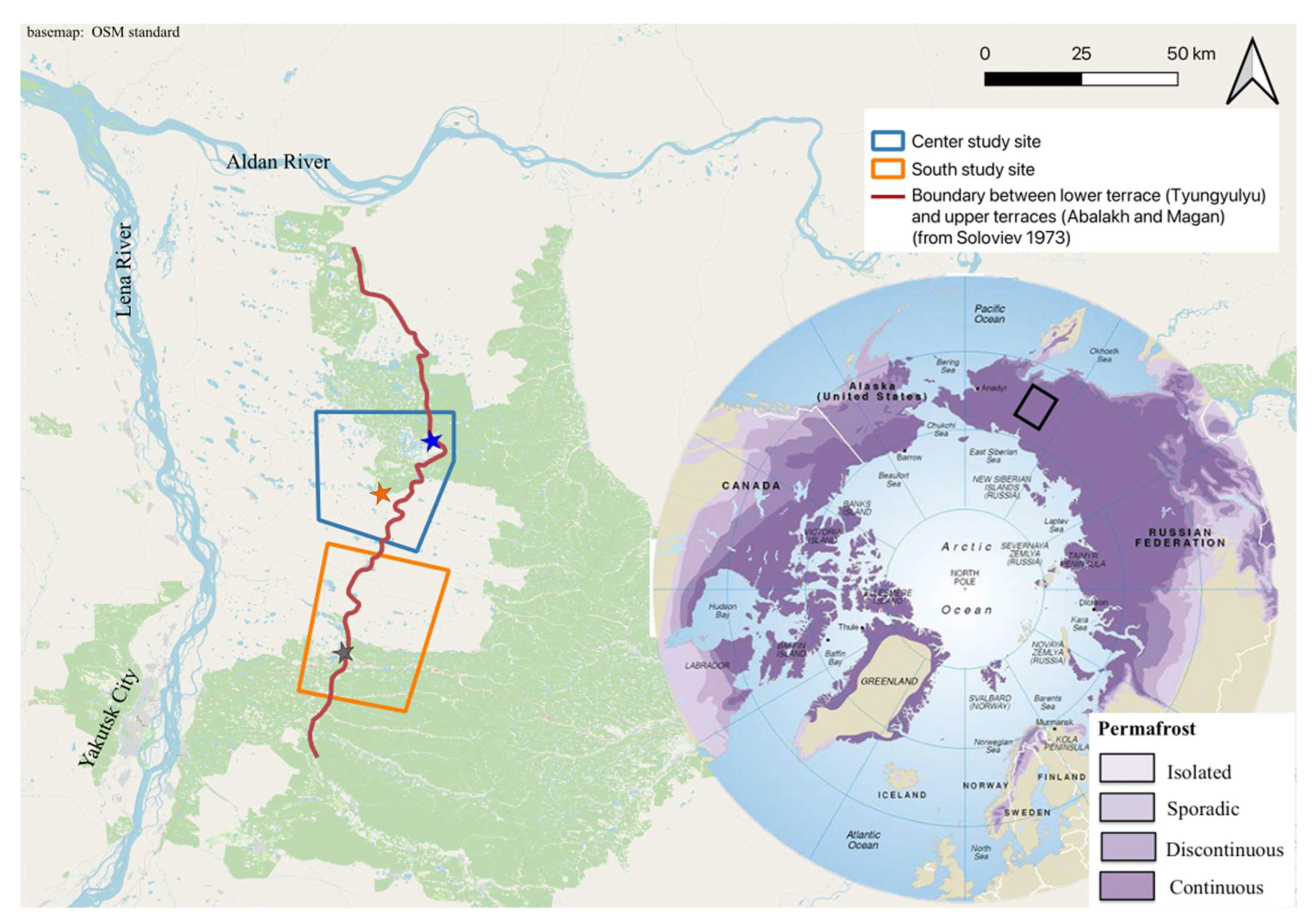
2.1. Study Site

Central Yakutia experiences an extreme subarctic continental climate with long, cold, and dry winters (January is the coldest month with a mean temperature around −40 °C) and warm summers (July mean temperature around +20 °C), causing strong seasonal variability [32]. The winter season (defined by the presence of ice cover on lake surfaces) usually lasts from early October until early May. Between 150–250 mm of precipitation accumulates each year, mostly during the summer months. Average snow depth for winter ranges from 24 cm in January to a maximum of 30 cm in March and then decreasing to 10 cm at the end of April (1980–2020 recorded values from Yakutsk weather station). The snow which falls in this region generally has very low water content due to cold temperatures [35] and yearly evaporation rates exceed total precipitation [35]. Central Yakutia, like other high latitude regions, is warming disproportionately faster than lower latitudes. Between 1996 and 2016, the mean annual air temperature of Central Yakutia increased by 0.5–0.6 °C per decade [36]. Spring snow cover has been disappearing 3.4 days earlier per decade (1972–2009) over the pan-Arctic terrestrial region and climate models predict decreases in snow cover duration between 10–20% by 2050 [37]. Changes in average snow depth and precipitation, however, are highly spatially heterogeneous with some areas of Eurasia experiencing increasing snow depth totals and precipitation [37].

Permafrost in Central Yakutia is generally continuous (Figure 1), thick (>500 m deep), and the upper 30–50 m (Pleistocene-age fluvial and aeolian sediments called ‘Yedoma’) can be extremely rich in ground ice (50–90% by volume) [38]. The amount of OC stored in Yedoma varies widely. For example, deep cores from Northern Siberia and Alaska yielded OC pool estimates of approximately 10 +7/−6 kg/m³ [39]. A 22 m deep core in Central Yakutia (Yukechi) on the Abalakh terrace yielded a much lower value of OC content of ~5 kg/m³ [40], while another Central Yakutian study (Spasskaya Pad/Neleger site) of a shallow core (2 m) showed a considerably higher OC content of 19 kg/m³ for the top two meters of larch forest covered Yedoma deposits [41].

The study site (62.55°N; 130.98°E) lies approximately 130 km north-east of the city of Yakutsk on a lowland plain between the Lena River to the west and the Aldan River to the east (Figure 1). The region is covered mostly by late Pleistocene sediments, including silty clays and sandy silts of fluvial, lacustrine, or aeolian origin [38]. Since the Pleistocene, numerous fluvial terraces have been formed from the activity of the Lena and Aldan rivers, and their smaller tributaries [42]. Two Pleistocene-age fluvial terraces underlay this region: the Tyungyulyu terrace, which covers the western section of the study area, 50–200 m above sea level (asl), dated 14–22 kyr BP, and the higher Abalakh terrace in the eastern sector of the study area, 200–280 m asl, dated 45–56 kyr BP [38,42]. This region is dominated by larch, pine, and birch forests and is characterized as a middle taiga landscape regime [35]. Grasslands are abundant in unforested areas, including land previously cleared for farming or ranching, or in the remnant depressions of old thaw lakes known as ‘alases’. They consist of halophytic steppe-like and bog plant communities [43].

Yedoma silty loams, which are common to the Lena-Aldan interfluve, underlay much of the study site, with abundant ground ice in the form of 1.5–3 m-wide ice wedges. Active layer depth in the region generally ranges between ~1 m below forested areas to >2 m in exposed grassland areas [44]. Zones of unfrozen ground (or taliks) exist underneath major rivers and lakes whose depth exceeds that of the ice cover in the winter. Nearly half of the landscape has been affected by thermokarst since the early Holocene, resulting in the formation of ~16,000 partly drained alas depressions [42,45,46]. However, recent thermokarst activity related to natural landscape evolution, increasing air temperatures, and/or human-induced landscape modifications (agriculture, clear-cutting, and infrastructure) is also widespread in the region. There are numerous small, recently developed, and expanding lakes and retrogressive thaw slumps along lake shores [47,48].

The thermokarst lakes in this region are divided into three categories based on field observations, past radiocarbon dating of lake sediments, geochemical signatures of lake waters, morphology, and a multiple-stage development model [6,16,39]. An illustrative example from the area is presented in Figure 2. Lakes of each type have strong differences in lake physiochemistry, dissolved GHG concentration, and GHG fluxes. The characteristic morphology of each lake type was determined from lakes with in-situ measurements and then applied to lakes in the remote sensing images. The morphology of each lake type is easily identifiable in the field and from remotely sensed images. The three lake types are as follows (illustrated in Figure 2):

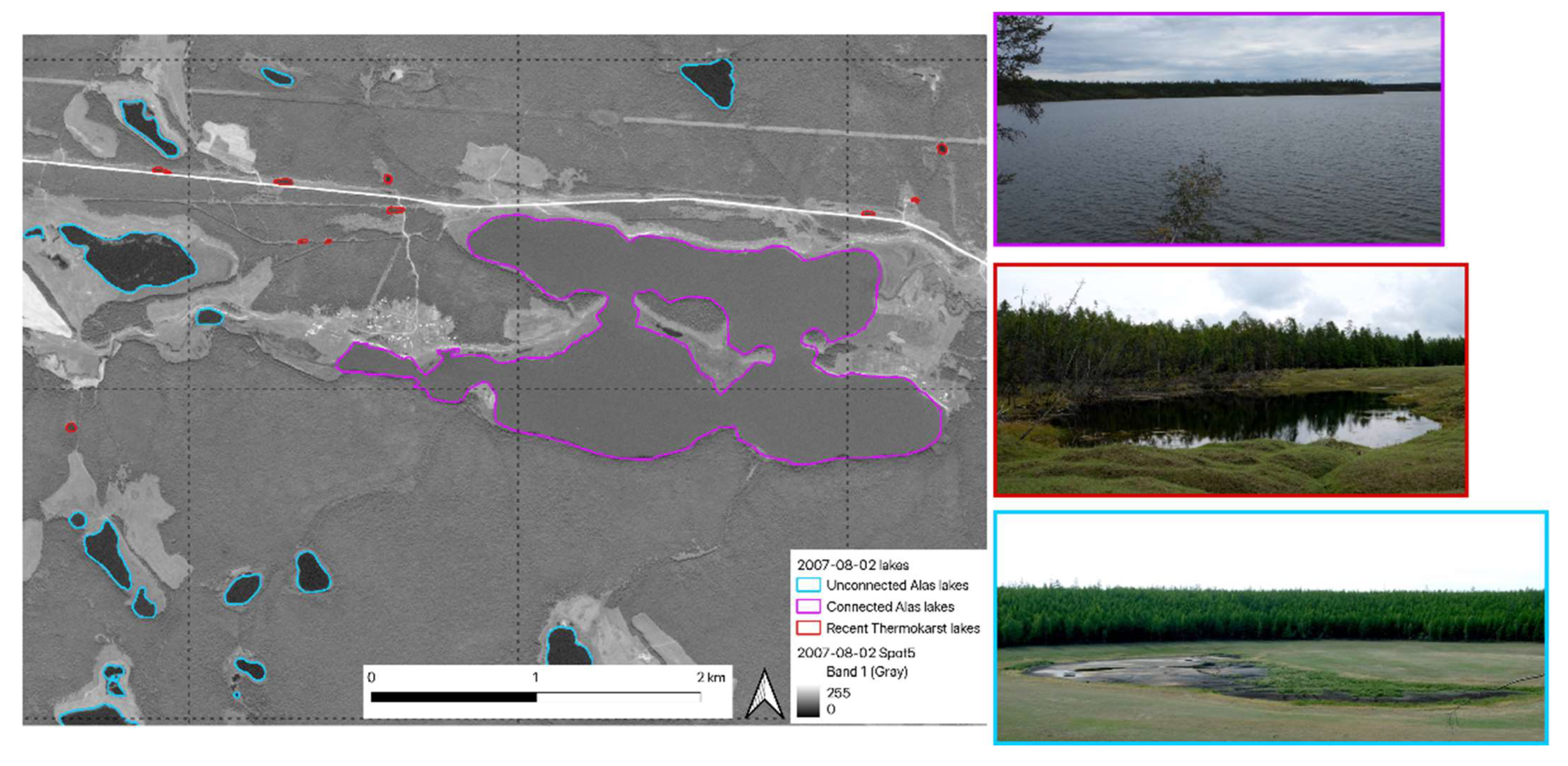
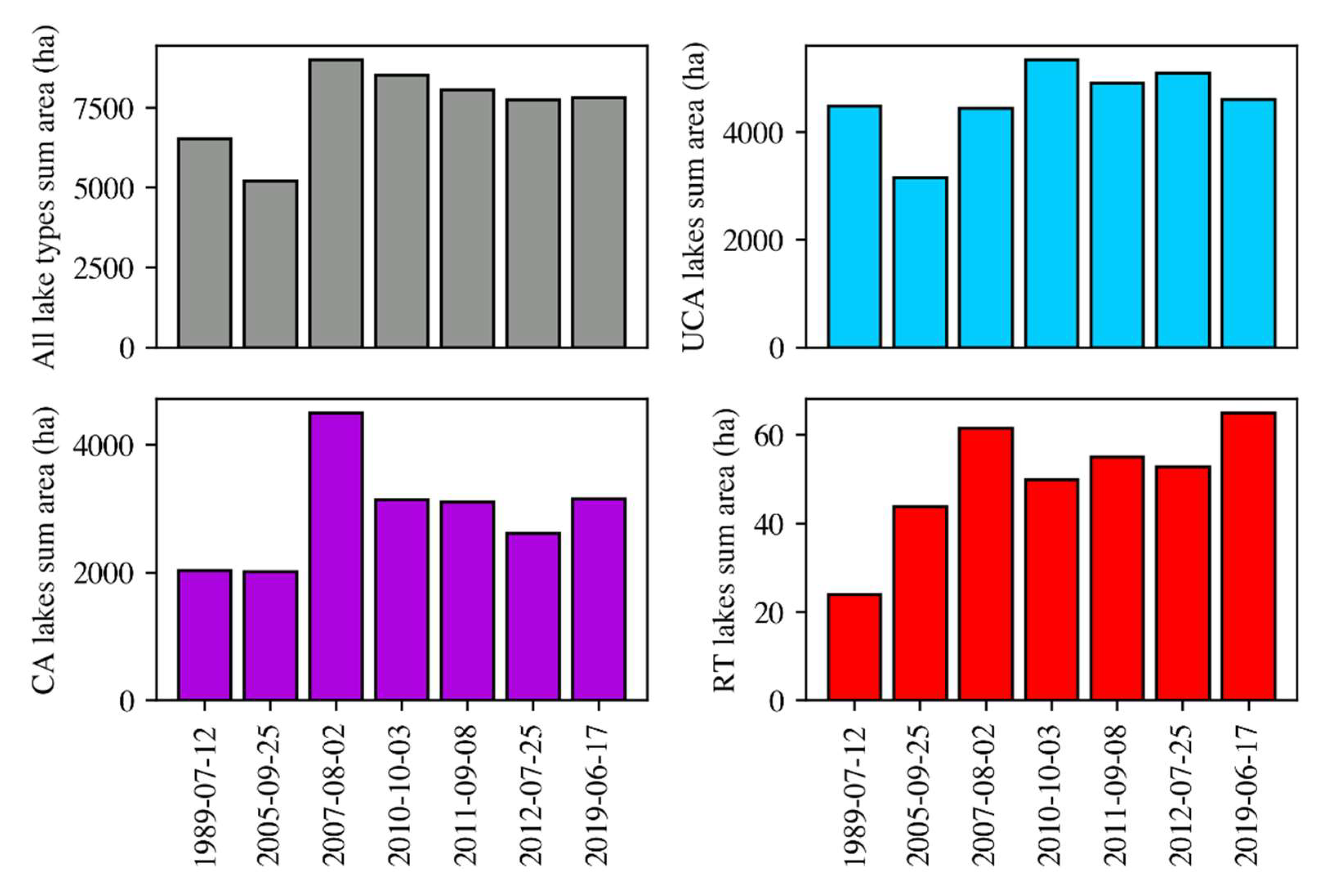
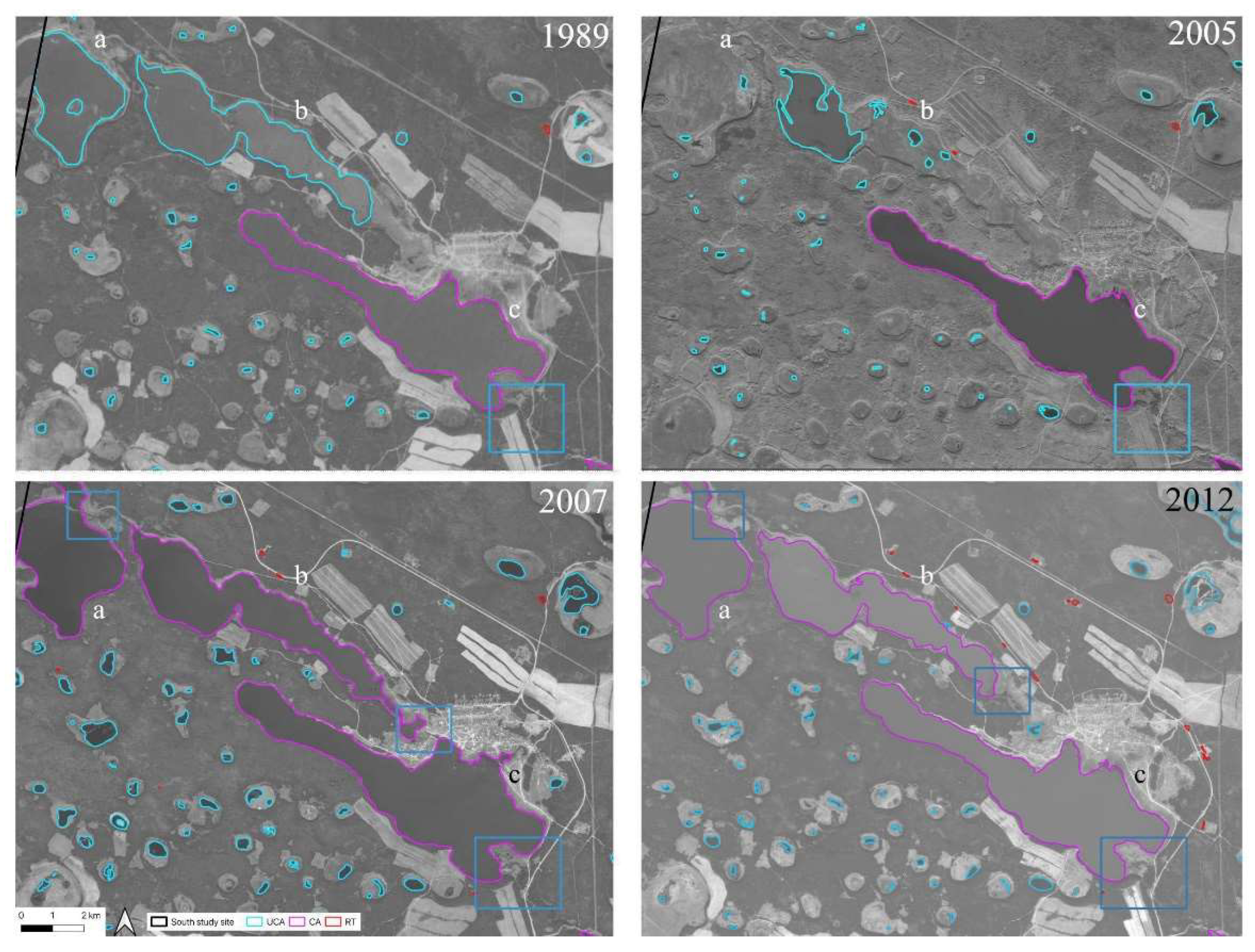
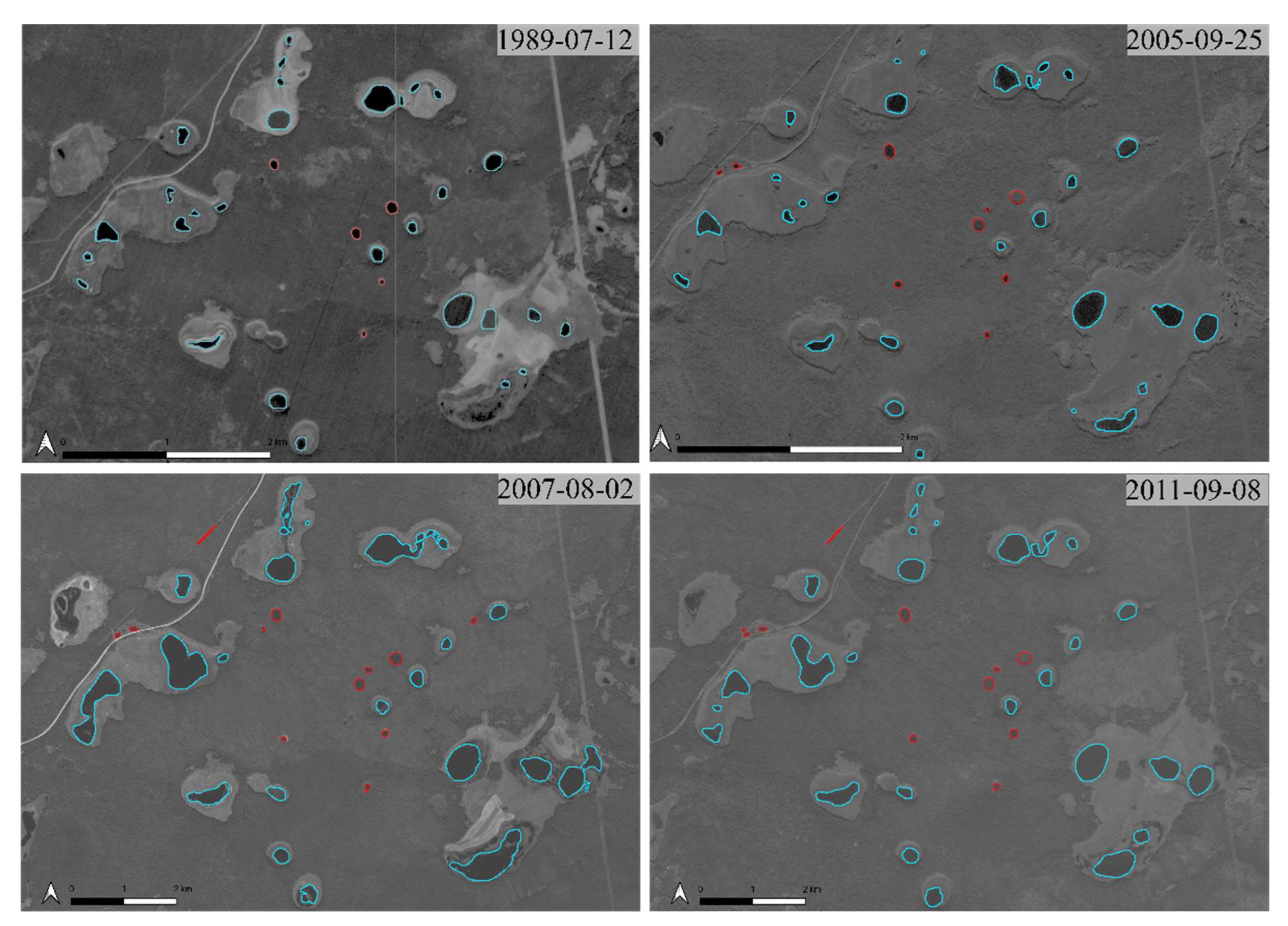
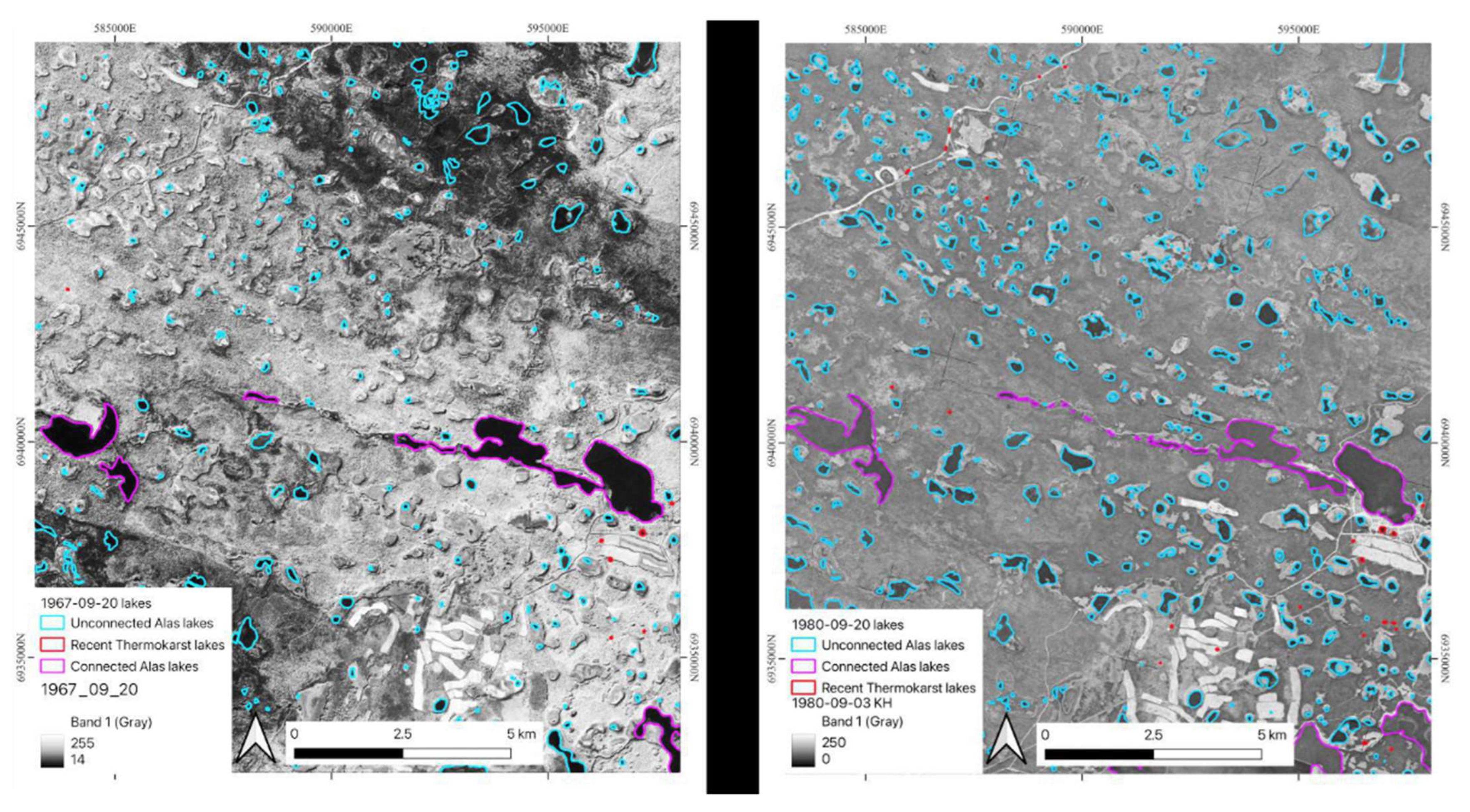
• Unconnected alas lakes: These are residual lakes located within hydrologically closed basins [16], which are represented in clear blue in Figure 2. Most of these lakes likely formed during the transition between the Pleistocene and Holocene, approximately 10–8 cal kBP or during the Holocene Thermal Maximum (~6.7–5 cal kBP) [43,49]. These lakes can be up to a few meters deep but are typically very shallow (1 m deep or less) and are usually completely frozen in winter. The ancient lake depressions surrounding the small residual lakes of this type can be up to several kilometers wide and several meters deep and are relatively easy to distinguish on satellite images. These alas lakes have already undergone much of the thermokarst processes and very little ground ice typically remains beneath the residual lake. Therefore, the thaw potential and resulting input of stored carbon to these lakes are low compared to recently formed thermokarst lakes [50].
• Connected alas lakes: These lakes, represented in magenta in Figure 2, are hydrologically connected to the watershed by streams or rivers. These lakes are consistently several hundreds of meters across and up to ~10 m deep. Most of them were probably formed during the mid-Holocene, approximately 5–3.5 thousand years ago, although detailed chronology about their inception is still incomplete [43,51].
• Recent thermokarst lakes: These lakes, in red in Figure 2, formed over the last several decades mostly from human activities (e.g., forest fire and forest removal for agriculture, pipelines, or road construction) and rising temperature [35,52]. These lakes are generally small (meters to tens of meters across) and relatively shallow (one to two meters deep) and are still expanding downwards and laterally due to active layer deepening and thermokarst processes. Compared to the other lake types, they have notably higher concentrations of dissolved OC [53].

2.2. Image Data Sources

In this study, we leveraged the entire archive of SPOT data available for the study region between 1986 and 2016 thanks to the SPOT World Heritage program. Developed by the Centre National d’Études Spatiales (CNES), the SPOT family includes five decommissioned satellites that operated between 1986 and 2015 (SPOT 1–5) and two operational satellites, SPOT 6 and SPOT 7, which were launched in 2012 and 2014, respectively (spatial resolution between 2–10 m) (Supplementary Table S1). The SPOT images were filtered to include only months between June and early October and a cloud cover of less than 70 percent. Many of the images which were taken between June and early October had very high percent cloud cover and could not be used for analysis. Frequent high percent cloud cover combined with a satellite return rate of 26 days resulted in a surprisingly small subset of exploitable scenes (maximum 10 images for any given area). Only single band, black and white SPOT images were available for use in this study.

We were able to augment this dataset slightly by including declassified military intelligence photographs (Supplementary Table S1). The declassified military satellite systems code-named CORONA, ARGON, LANYARD, and Hexagon operated between 1960–1986 collecting photographs of the USSR and China. The data were downloaded from the USGS website (EarthExplorer). These black and white images were not georeferenced (spatial resolution ~2.5 m). Manual georeferencing was done in QGIS 3.16 [54].

2.3. Defining Lake Boundaries and Lake Types

It was often clear which pixels belonged to the lake surface or to the surrounding dry land. In the instances where the water/land boundary was ambiguous, every effort was made to include all liquid water associated with the lake. However, it was sometimes unclear whether darker pixels surrounding a lake were liquid water or heavily saturated mud (Figure 3). In these cases, best judgment was used to include all pixels which correspond to the lake area. Some subjectiveness is inherent in this process. Frequently, unconnected alas lakes develop into a half moon shape or a peripheral ribbon of liquid water surrounding dry ground (Figure 4). In these cases, only the liquid water was included in the lake area.

Using QGIS, lake type classification was manually assigned to the lake outlines. In the absence of in-situ measurements, lake type classification was determined based on the characteristic lake morphology determined from lakes where in-situ measurements exist. Connected Alas (CA) lakes were easily identified based on their generally large size and the presence of inflow and/or outflow rivers and streams (see the CA lake in magenta in Figure 2). Some CA lakes experienced such significant surface area reduction in some years that they were reclassified as Unconnected Alas lakes (UCA) for those particular scenes. UCA lakes were identified based on their characteristic surrounding dry depression (Figure 2). The size of these depressions varies from year to year and from lake to lake depending on precipitation levels, the lake’s phase in the multiple-stage development model, and surrounding topography. Recent Thermokarst (RT) lakes were generally small and directly surrounded by forest or other vegetation cover (Figure 2). For a small number of lakes (<10 in each scene), it was difficult to determine whether it was an UCA lake or a RT lake. In these cases, lake morphology and the surrounding environment were carefully considered, and the best guess decision was made.

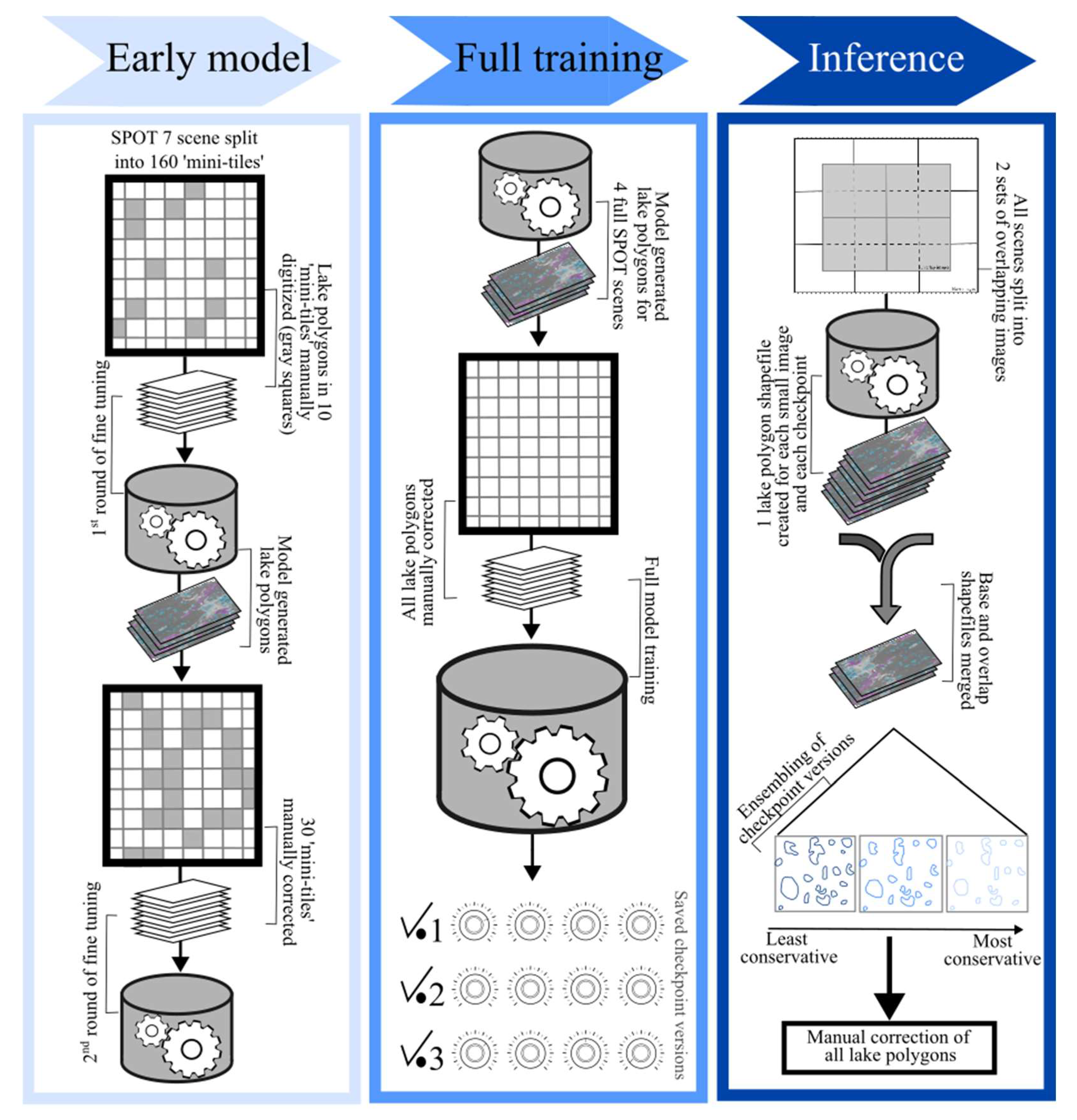
2.4. General Deep Learning Workflow

2.4.1. Machine Learning Model

This project used deep learning techniques, specifically Mask Region-Based Convolutional Neural Networks (R-CNN) instance segmentation, to automate lake detection in satellite images of Central Yakutia. Mask R-CNN is a deep learning instance segmentation method that is used to identify different objects in an image (i.e., pedestrians on a sidewalk, animals in a field, etc.) [34]. Our implementation builds on top of the existing reference PyTorch implementation [55]. The backbone of the neural network is ‘resnet50’ [56].

The neural network can receive an input image between 800–1333 × 800–1333 pixels. Each satellite image, however, is approximately 30,000 × 30,000 pixels. Therefore, every satellite image was split into ~900 smaller images (depending on the original image size) and the neural network treated every image separately. This resulted in lake predictions which exhibited undesirable artifacts. For example, a lake spanning two or more small images was artificially divided into smaller polygons. To alleviate this problem, each scene was split a second time into ~900 smaller images. These images were positioned in a staggered overlap of the ‘base’ images such that the corners of these ‘overlapping’ images were in the middle of each of the base images (Figure 5). Each of the image sections (base and overlapping) were treated identically by the model. This process facilitated the fusing of lake polygons which spanned multiple small images into single polygons.

2.4.2. Fine Tuning and Training

The workflow for fine-tuning and training of the deep learning model included a three-step process of initial fine tuning using a very limited data set, a second round of fine tuning using a substantially larger dataset, and lastly, the full model training using four complete scenes (Figure 6). The first step was the fine tuning of the model using a limited amount of data to get preliminary results. The fine-tuning dataset was created using a SPOT 7 image (11 September 2016). The original image was split into 160 smaller images (1024 × 1024 pixels), hereafter referred to as ‘mini-tiles’. Ten of the mini-tiles were chosen, and all lake polygons in the image were manually digitized. The digitized lake polygons were then used as a preliminary fine tuning of the model. After fine tuning, the model was run to generate lake polygons for the mini-tiles. Thirty mini-tiles were randomly chosen, manually corrected, and used as a second round of fine tuning of the model. The twice fine-tuned model was then used to generate polygons for four complete SPOT images. The lake polygons for the four images were then manually corrected and used to complete a full training of the neural-network (

Table 1. Description of scenes used for full training. The ‘number of lakes’ was determined by a combination of automatic polygon generation and manual corrections.

Scene Date	Satellite	Scene Area (km2)	Pixel Area (m2)	Number of Lakes
2016-09-11	Spot 7	35 × 43	1.5	2525
2012-09-25	Spot 5	60 × 60	2.5	4197
2010-10-03 N	Spot 5	60 × 46	2.5	1210
2010-10-03 S	Spot 5	60 × 14	2.5	1413

).

From the four fully annotated SPOT images, a training dataset of 8286 training samples was created. Each training sample consisted of a 1-megapixel image. Standard data augmentation practices were followed (random rotation, scaling, and brightness adjustment). The Adam optimization algorithm was used to train the model [57]. For each of the 8286 1-megapixel images, the training of the neural network spanned 50 epochs, and checkpoints were saved after every epoch. Each checkpoint is a set of neural network parameters (‘weights’).

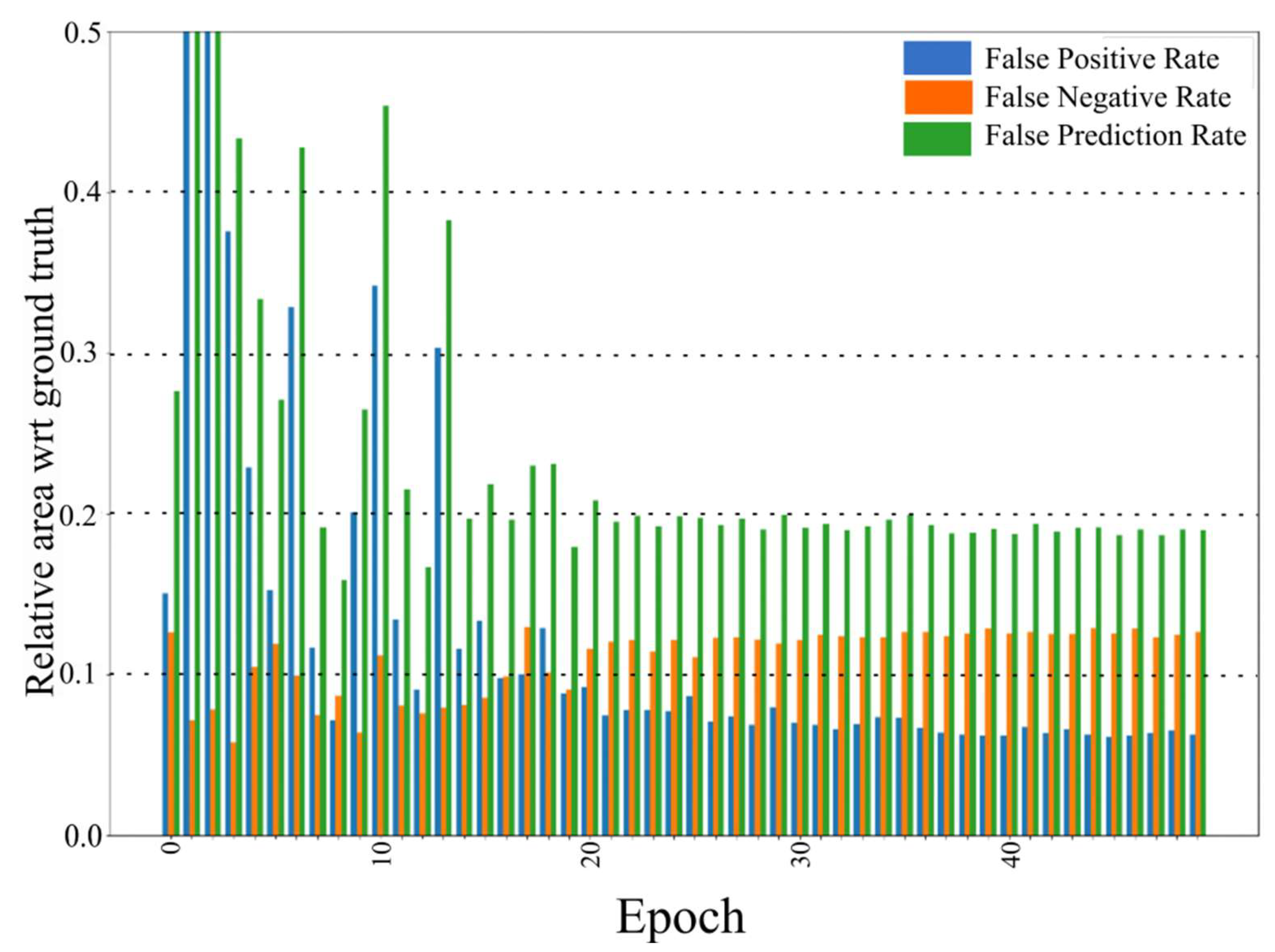
2.4.3. Accuracy Assessment of Model

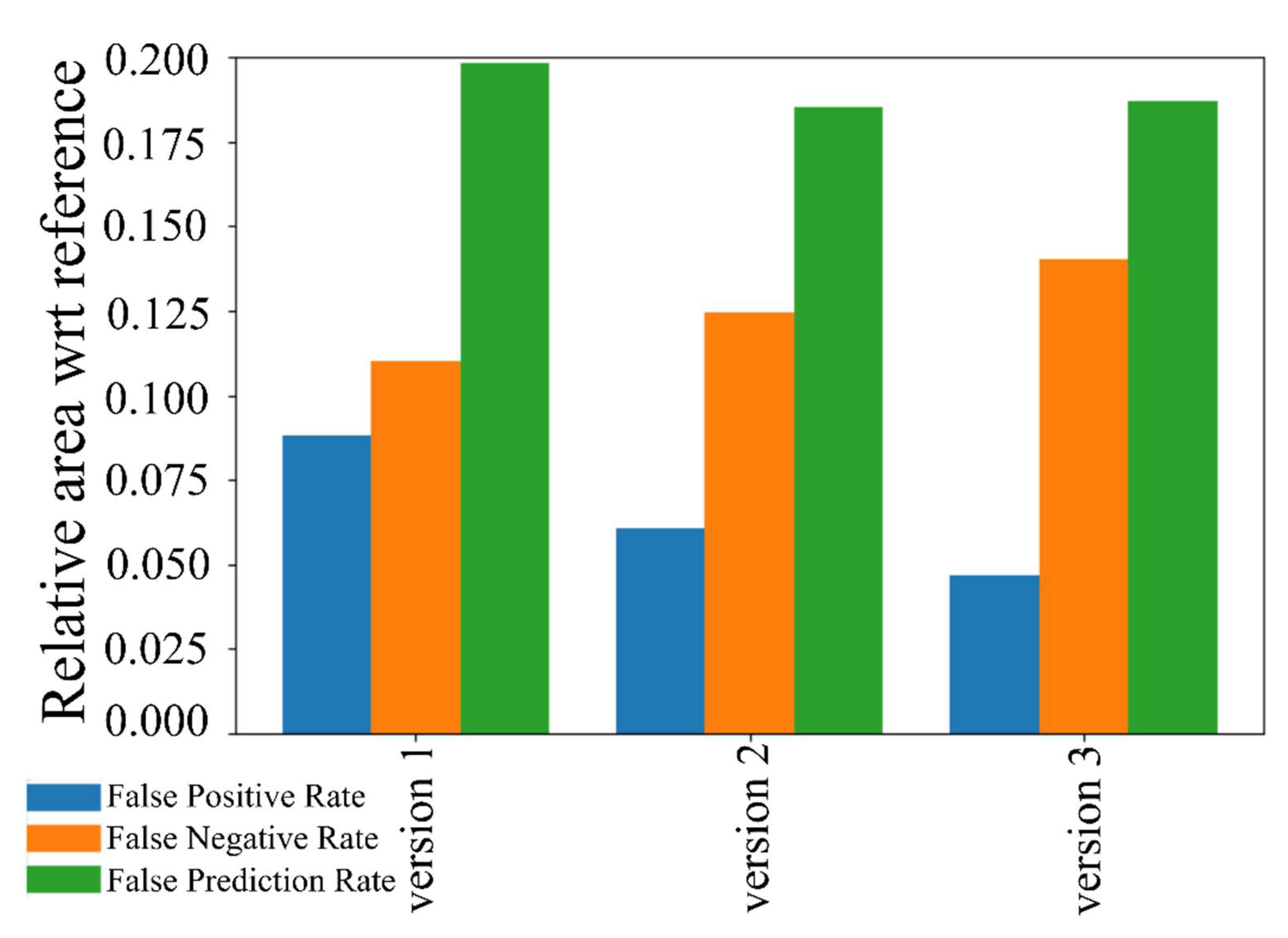
In order to assess the accuracy of the predicted lake outlines, the lake outlines generated by the 50 checkpoints were compared to the manually corrected lake outlines. The false positive rate (a lake polygon was predicted where no lake exists) and false negative rate (no lake polygon was predicted where a lake exists) were calculated. The false prediction rate is the sum of the false positive rate and the false negative rate. The relative error in the total predicted lake area is the difference between the false positive and negative rates, which is therefore less than the false prediction rate. Figure 7 shows the evolution of these errors as the training progresses. The training can be divided into two phases: a first phase (epochs 0–20) where the prediction error decreases from a >50% rate to a ~20% rate, and a second phase (epochs 20 and up) where it stabilizes in the 17 to 20% range.

2.4.4. Ensembling

In order to improve the error rate of the initial model, an “ensembling” technique was developed which leveraged the variability in predictions of the different training states. This technique enhanced the accuracy and robustness of the model. Three sets of weights were manually chosen from the second half of the training (epochs 25–50 in Figure 7 and used to generate the three final lake polygon versions using ensembling. The weights were chosen from epochs after 25 because this is where the predicted area with respect to ground truth levels off at ~20% and remains stable for the subsequent training epochs (Figure 7). Ensembling is the aggregation of the three manually chosen prediction layers as follows: the first lake polygon prediction contains all polygons generated by all three saved weights (herein called ‘version 1’; least conservative). The second lake polygon prediction contains all polygons predicted by at least two of the saved weights (‘version 2’). The third lake polygon prediction contains only polygons which were predicted by all three of the saved weights (‘version 3’; most conservative). The three polygon versions are ‘nested’. Version 1 includes all the polygons which are also included in version 2 and version 3. Version 2 contains all polygons which are also included in version 3. The lake outlines generated by the ensembling technique improved slightly upon the initial model predictions (Figure 8). However, three lake outline shapefiles (spatial dataset file which holds all of the lake outlines for each of the three ‘versions’) generated by the ensembling technique made manually correcting the lake outlines simpler and more efficient. Lakes which were not predicted in one of the ensemebled shapefiles could generally be found in one of the other two shapefiles, eliminating most instances of manually digitizing an entire lake.

2.4.5. Comparison of Total Surface Area for Prediction and Corrected Lake Outlines

To determine whether one of the ensemble versions could be used for lake surface change analysis without manual correction of the lake outlines, three entire lake outline shapefiles (2011-09-08; 2011-09-21; 2013-07-14) were manually corrected to assess the differences between the predicted total lake surface area of each of the three versions to the manually corrected total lake surface area. The manual corrections utilized the lake polygons generated by the neural network, but were rectified where needed. Manual digitizing, as was done in the first stage of fine-tuning the neural network, is extremely time-consuming and tedious. Manually digitizing one 60 × 60 km² scene without the aid of the polygons generated by the neural network takes at least one full week of motivated work. Correction of the polygons generated by the neural network for one scene could be completed in two–three hours or less. Version 1 consistently over predicted total lake surface area (+2.7–+8%; +556–+1648 ha false prediction rate). Version 2 under predicted the total surface area for two out of the three corrected scenes (−9–+4%; −1853–+824 ha false prediction rate). Version 3 under predicted two out of the three corrected scenes (−12–+0.5%; −2471–+103 ha false prediction rate). Based on these results and the reduced time to manually correct the neural network lake outline shapefiles, the decision was made to manually correct all the lake outline shapefiles used in the lake surface area change analysis.

2.5. Surface Area Change Analysis

The available scenes were separated into two study areas to facilitate lake surface area change analysis: center and south (Figure 1). These study sites were drawn to maximize the temporal and spatial coverage of available scenes and to include all three lake types. All lakes with available in situ measurements (as presented by [6] and compiled in [51] are within the center study site (Figure 1). Lake type assignment followed the same method as described above. Lake outlines generated by the neural network were manually corrected and used to calculate lake surface area for all analyzed scenes. Overall lake surface area and lake surface area by lake type were then compared between scenes for each study site. Changes in lake count are not discussed in this study because it does not necessarily reflect an actual increase in lake number. This is particularly true for UCA lakes as a lake which was digitized as a single polygon in one scene may be represented by several smaller polygons in a subsequent scene if the lake has experienced a reduction in surface area and the smaller residual waterbodies are no longer connected.

2.5.1. South Study Site

Lake surface area was compared between seven scenes spanning 1989–2019. The scenes are not evenly distributed in time and there is a large gap between 1989 and 2005. Image acquisition months range from mid-June to early October. The south study site covers an area of 1220 km² and there is substantial human activity present in the scene, particularly in the western half of the scene (pastoral practices, villages, and numerous roads) (Figure 1). The City of Balyktakh (Балыктах) (population ~900 from 2010 census) is located in the lower half of the scene near the middle. Approximately 80 percent of the study site lies on the Tyungyulyu terrace and the rest on the Abalakh terrace [9,13,42]. Lake surface area comparison is based on seven scenes from 1989–2019. The scenes are not evenly distributed in time and there is a particularly large gap between the 1989 scene and the next scene in 2005 (

Table 2. Dates of scenes and satellite platform used in each study site.

South (1220 km2)	Satellite	Center (1150 km2)	Satellite
1989-07-12	Spot 1	1967-09-20	KH-4 Corona
2005-09-25	Spot 5	1980-09-20	KH-9 Hexagon
2007-08-02	Spot 5	2010-09-23	Spot 5
2010-10-03	Spot 5	2011-09-21	Spot 5
2011-09-08	Spot 5	2012-07-25	Spot 5
2012-07-25	Spot 5	2016-09-11	Spot 7
2019-06-17	Spot 6	2019-06-17	Spot 6

).

2.5.2. Center Study Site

Lake surface area was compared between seven scenes spanning 1967–2019 in an 1150 km² study area (Figure 1; Table 2). The scenes are not evenly distributed in time and there is a large gap between the 1980 (September 20) scene and the 2010 (September 9) scene (Table 2). Image acquisition months range from mid-June to September. The City of Borogontsy (population 5222 from 2010 census) and the Village of Syrdakh (population ~800 from 2010 census) are the largest populated areas in the scene. Approximately 80 percent of the study site lies on the Magan terrace and the rest on the Tyungyulyu terrace [9,13,36]. The large UCA lake near the City of Borogontsy (indicated by the blue star in Figure 1) was not included in these analyses. The water level of this lake are manually controlled by the inhabitants of Borogontsy and is therefore not representative of the natural response of lakes to changes in temperature and precipitation (A. Fedorov (Melnikov Permafrost Institute) pers. comm.). Additionally, the complex morphology of this lake was not well predicted by the algorithm for any scene and manual correction of the lake was time-consuming and laborious.

2.6. Temperature, Precipitation, and Evapotranspiration

An exceptionally long record of temperature and precipitation data is available from the meteorological station of Yakutsk (World Metrological Organization Index: 24,959; 62.0866°N, 129.7500°E) (1888–present). These data were compiled from daily records to monthly sums (precipitation) and monthly averages (temperature) from 1960–2020. To account for all precipitation that might have influenced lake surface area (e.g., snowfall), we used the hydrologic year, i.e., the year start date was shifted to 1 October of the previous year. For example, for a scene taken on 1 September 2000, the yearly precipitation would have included precipitation data from 1 October 1999 to 31 September 2000. These data were then compared to a 30-year moving average (minimum window 10 years). Reference evapotranspiration was calculated using the Blaney-Criddle Method [58], which uses daily mean temperature and mean daily percent of annual daytime hours. The Mann-Kendall Trend test was used to determine whether any trend existed in the temperature, precipitation, and evapotranspiration data. All analyses were completed using the Python programming language (Python Software Foundation, http://www.python.org/, accessed on 1 February 2023).

3. Results

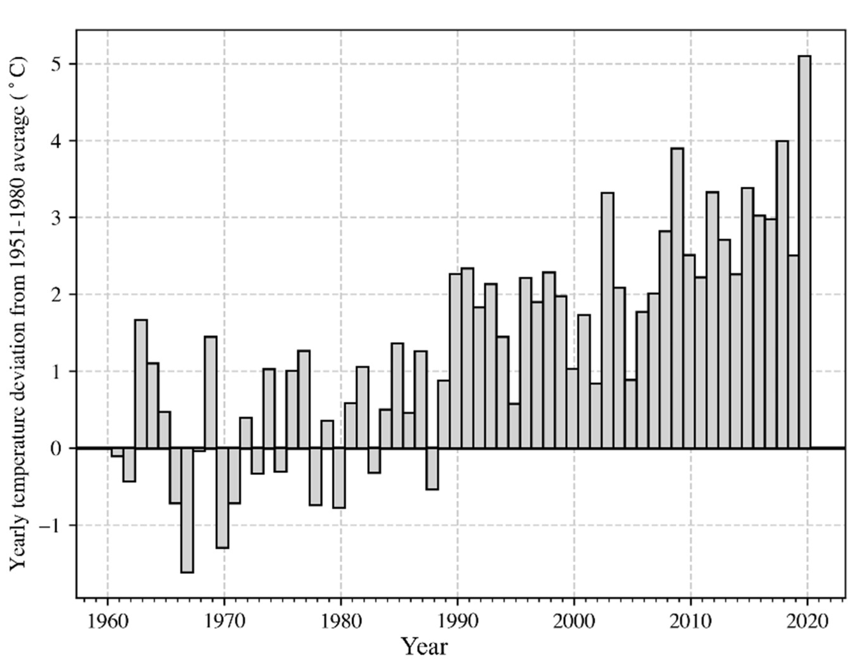
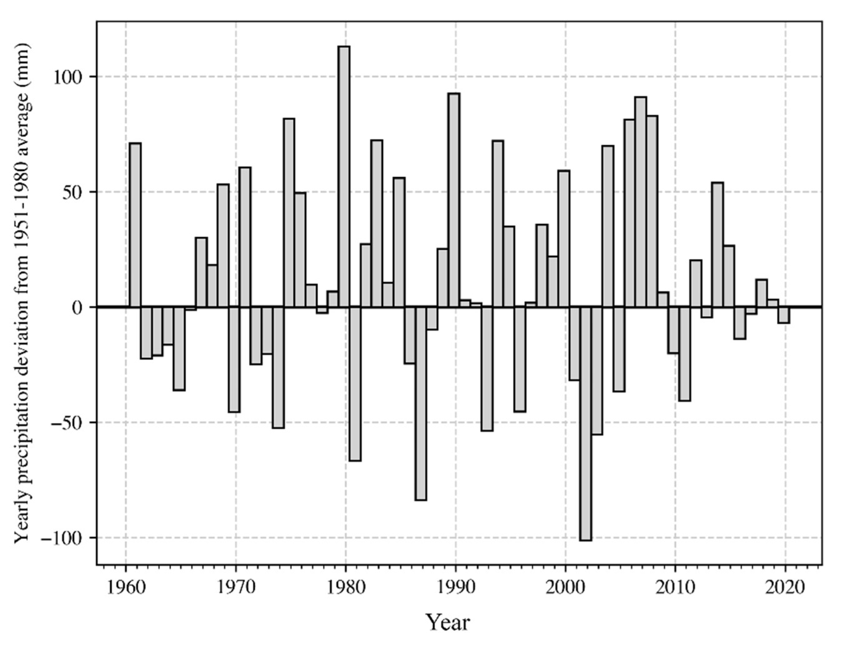
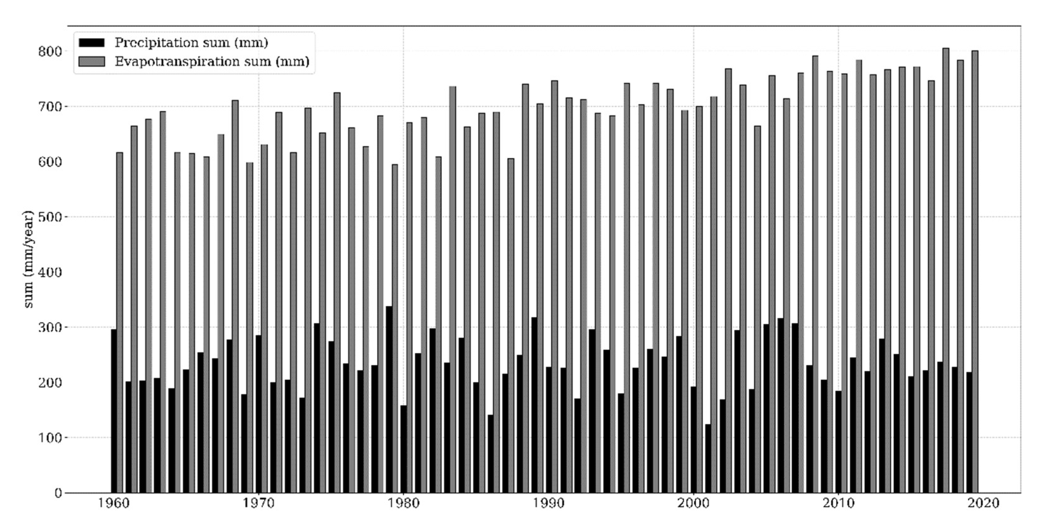
3.1. Trends in Temperature, Precipitation, and Evapotranspiration since 1900

Temperature records from the Yakutsk station (62.0866°N, 129.7500°E) show an increasing frequency of years with above average annual temperatures, especially after the late 20th century, and an overall trend of increasing temperature (Mann Kendall test: trend = increasing; p = 1.31 × 10⁻¹¹) (Figure 9). The mean annual air temperature (MAAT) in 1900 was −14.6 °C and the MAAT in 2019 was −5.3 °C. The years after 1990 exhibit particularly consistent above average MAAT (average MAAT 1951–1980: −10 °C; average MAAT 1990–2019: −8 °C). The temperature records from Yakutsk station and other sites (e.g., [37]) indicate a decadal temperature increase of 0.7 °C since 1900. There is no observable trend in yearly precipitation in Central Yakutia (Mann Kendall test: no trend; p = 0.813) (Figure 10). Yearly average evapotranspiration in Central Yakutia shows an increasing trend (Mann Kendall test: trend = increasing; p = 1.69 × 10⁻¹²) (Figure 11).

3.2. Spatial Distribution of Lake Types

Based on the 2019 (June 17) scene, the limnicity of the center and south study sites were 9% and 5%, respectively. A large proportion of the center study site (~80 percent) is situated on the lower-lying and younger Tyungyulyu terrace while the remaining ~20 percent lies on the higher and older Abalakh terrace. The south study site has approximately the inverse proportions on the Tyungyulyu and Abalakh terraces, likely contributing to the differences in limnicity between the two study sites. Ulrich et al. [13] also found a higher density of lakes on the Tyungyulyu terrace compared to the Abalakh terrace.

In both study sites and every scene, unconnected alas (UCA) lakes were by far the dominant lake type in both count and total surface area (

Table 3. Lake type statistics based on the 2019 (June 17) scene.

	Lake Type	Min Area (ha)	Max Area (ha)	Median Area (ha)	Mean Area (ha)	Count
South	UCA	0.01	1816.4	5.1	17.4	1212
	CA	7.9	2178.7	179.5	517.7	28
	RT	0.1	17.7	1.0	1.8	165
Center	UCA	0.01	94.5	0.9	2.9	1486
	CA	0.02	237.7	7.1	44.7	43
	RT	0.01	13.9	0.2	0.4	323

). The mean surface area for UCA lakes in the center study site was 3.0 ha, which is consistent with the findings of [6] (Table 3). The mean surface area for UCA lakes in the south study site was 17.4 ha (Table 3). There are approximately five lakes in each study site which transition from CA to UCA, and vice versa, between some years. These lakes were widely distributed throughout each scene. UCA lakes in both study sites have a nearest neighbor index value slightly lower than the value expected for randomly distributed objects (south study site UCA nearest neighbor index: 0.73, z-score: −17.6; center study site UCA nearest neighbor index: 0.79, z-score: −14.9). The nearest neighbor index is the ratio between the observed and expected average nearest neighbor distance. A nearest neighbor index close to zero indicates point clustering. A nearest neighbor index near or greater than one suggests random or uniform distribution, respectively. The z-score indicates the level of confidence, with the higher absolute value being more significant.

Connected alas (CA) lakes were the least numerous, but second in terms of total surface area. The average surface area of CA lakes was 517 ha and 48 ha for the south and center study sites, respectively. CA lakes were generally much larger than either RT lakes or UCA lakes (Table 3). The center study site had the most CA lakes (~45), while the south study site had ~30. These lakes also have a nearest neighbor index value slightly lower than the value expected for randomly distributed objects (south study site CA nearest neighbor index: 0.79, z-score: −2.1; center study site nearest neighbor index: 0.68, z-score: −3.2).

Recent thermokarst (RT) lakes were the second most abundant lake type in terms of count, although they accounted for proportionally less of the total surface area due to their generally small size (Table 3). The mean surface area for RT lakes in the center study site was 0.4 ha and 1.8 ha in the south study site (Table 3). RT lakes exhibited the strongest spatial clustering based on the nearest neighbor analysis (south study site nearest neighbor index: 0.52 z-score: −11.8; center study site nearest neighbor index: 0.53, z-score: −16.0). Although some RT lakes do appear to have formed in the absence of any human disturbance (Supplementary Figures S1–14), most of these lakes form within 1–2 km of roads or cleared land for pastoral practices or infrastructure development. Clusters of RT lakes can be seen, for example, near the City of Borogontsy and the village of Syrdakh (in the center study site).

3.3. Lake Surface Area Change: South Study Site

The 1989 (July 12) and the 2005 (September 25) scenes had the lowest overall lake surface area with 2005 being slightly lower than 1989 (Figure 12 and Figures S1–S7). Total surface area increased substantially from 2005 to 2007 (August 2) and decreased in the next three available scenes (2010-10-03, 2011-09-08, and 2012-07-25). The 2019 scene (June 17) had nearly the same total surface area as the 2012 (July 25) scene. Changes in UCA lake surface area drive the trend in overall lake surface area, as they are the most numerous lake type and make up the largest proportion of the total surface area. UCA lake surface area is significantly negatively correlated to yearly average precipitation (Spearman coefficient = −0.82, p value = 0.02;

Table 4. Spearman coefficient values and p values related to the correlation of lake surface area with precipitation, temperature, and evapotranspiration. p-values < 0.05 are in bold. The datasets used are smaller than generally acceptable for robust correlation testing (>30 samples).

	Lake Type	Precipitation		Temperature		Evapotranspiration
		Coefficient	p-Value	Coefficient	p-Value	Coefficient	p-Value
South	UCA	−0.82	0.02	0.46	0.29	0.61	0.15
	CA	−0.46	0.29	0.71	0.07	0.68	0.09
	RT	−0.36	0.43	0.86	0.01	0.89	0.01
Center	UCA	−0.29	0.53	0.04	0.94	0.18	0.70
	CA	−0.29	0.53	0.29	0.53	0.29	0.53
	RT	0.54	0.22	0.82	0.02	0.79	0.04

). This is likely due to several large UCA lakes changing lake type designation from UCA lakes to CA lakes during years of high precipitation and the re-establishment of inflows and outflows (see discussion section below). RT lake surface area peaked in 2007 and decreased slightly in subsequent scenes before a higher peak in the 2019 (June 17) scene. RT lake surface area is significantly positively correlated to temperature (Spearman coefficient = 0.86, p value = 0.01; Table 4). The surface area of CA lakes peaked in 2007 and decreased in 2010, with the surface area remaining stable in subsequent scenes. CA lake surface area is not significantly correlated to any of the three weather variables (Table 4). It is important to note that the datasets used in this study are smaller than generally acceptable for robust correlation testing (>30 samples) and the results of the Spearman correlation test should be considered only as possible indications of significant or insignificant correlation.

At a smaller scale (i.e., <10 km²), we see that the surface area of some lakes can change drastically from year to year. Between some scenes in the south study site, a significant reduction and/or disappearance of lakes is observed. For example, two large UCA lakes (surface area lake a = 212 ha, b = 280 ha) which are visible in the image from 1989 (July 19) experience significant surface area reduction in the 2005 (September 25) image (Figure 13). Lake a in Figure 13, disappeared almost completely while lake b lost approximately 50 % of its surface area: from 268 ha in 1989 to 134 ha in 2005. A proximal CA lake (lake c) however, maintained an almost equal surface area between 1989 (403 ha) and 2005 (446 ha). It is likely, based on field observations of similar lakes, that lake c is deeper than either lake a or b. In situ measurements from [6] of lakes in the center study site showed that CA lakes are generally much deeper than UCA lakes (mean CA depth = 5.7 m; mean UCA depth = 2.2 m). As soon as 2007 (August 2), the two UCA lakes had regained their previous extents (surface area lake a = 403 ha, b = 309 ha, lake c = 461 ha) (Figure 13). Lake a even merged with the UCA lake slightly to the northwest. CA lake c maintains a consistent surface area compared to the two UCA lakes.

A slightly different trend is visible approximately 13 km north in the south study site during the same period. A comparison of approximately 30 small UCA lakes between 1989 (July 12) and 2005 (September 25) indicates a negligible change in surface area (surface area UCA lakes 1989 = 44 ha, 2005 = 43 ha; Figure 14). There is an increase in the number of RT lakes from five in 1989 to 11 in 2005 and an increase in RT lake surface area from 2.5 ha in 1989 to 4.0 ha in 2005. Three small RT lakes appear north of the road which bisects the left corner of the 2005 image in what appears to be a newly cleared field. A fourth RT lake appears parallel to the straight road just north of the meandering road. By 2007 (August 2), the surface area of UCA lakes had increased to ~100 ha and the number of RT lakes had increased to 12 and surface area to 5 ha. In 2011 (September 8), UCA lake surface decreased slightly to 62 ha and RT lake surface area increased to 5.2 ha.

3.4. Lake Surface Area Change: Center Study Site

The 1967 (September 20) scene had substantially lower total lake surface area compared to the other six scenes (Figure 15 and Figures S8–S14). In the 1967 scene, many alas basins are occupied only by a very small, residual lake or no lake at all (Figure 16). 1967 CA lake surface area values are closer to those of the other six scenes. By the 2010 (September 23) scene, many of these alas depressions are again occupied by more substantial lakes compared to the 1967 scene (Figure 16). Total lake surface area peaks in 2010 and decreases throughout the subsequent scenes. UCA lake surface area follows the same trend as overall lake surface area. CA lake surface area remains mostly stable except for an exceptionally high value in 1980 (September 20). The high CA lake surface area value for this scene is related mostly to a single large lake (indicated by the black arrow in Supplementary Figure S9). By 2010, this lake had lost approximately half its surface area (becoming an UCA lake) and is relatively non-existent in subsequent scenes. There is an overall trend of increasing RT lake surface area through time, in contrast to UCA lakes, which display a decreasing trend through time. RT lake surface area in this study site is positively correlated with temperature and evapotranspiration, while UCA and CA lake surface areas do not show a statistically significant correlation with any of the three weather variables (Table 4).

4. Discussion

The results of this multi-decadal lake surface area change analysis indicate that there are strong differences in the spatial distribution of the three lake types and their responses to changes in temperature, precipitation, and evapotranspiration. In general, there are slight trends of decreasing UCA lake surface area, stable CA lake surface area, and increasing RT lake surface area. At a smaller scale (i.e., <10 km²), the surface area of some lakes can change drastically from year to year, which has implications for local hydrology and water availability for surrounding populations.

4.1. Alas Lake Dynamics and Environmental Variables

The observed trend of decreasing UCA lake surface area compared to increasing RT lake surface area and stable CA lake surface area is likely related to differences in lake morphology and related dynamics between the three lake types. Lake type response to changes in temperature, precipitation, evapotranspiration, and possibly other variables that are beyond the scope of this study likely also play a role in the observed surface area trends. UCA lakes are generally no longer surrounded by ice-rich permafrost [47,48,59]. After the initiation of thermokarst processes, the active layer beneath a lake can reach substantial depths as heat absorbed into the lake during the summer is transferred into the surrounding ice-rich permafrost, perpetuating permafrost thaw even during winter months. Eventually, a talik (an area of constantly thawed ground) forms beneath the lake. Heat transfer between the lake, talik, and surrounding permafrost creates a positive feedback cycle of lake expansion and permafrost thaw [59]. Once all the surrounding permafrost has been thawed, the lake’s surface area is controlled primarily by evaporation and precipitation, as is the case for UCA lakes in the study areas. Both evapotranspiration and precipitation rates have increased in Central Yakutia since 1960, but evapotranspiration substantially exceeds precipitation in this region (Figure 11) (this study and [35]). Although no strong statistical correlation was observed between UCA lake surface area and any climate variable, it is likely that increasing evapotranspiration is contributing to decreasing UCA lake surface areas. Crate et al. [46] found that the water level of an unconnected alas lake (Tyungyulyu alas lake) was correlated with the warm season (May to September) air temperature and corresponding evapotranspiration. UCA lakes are more susceptible to evapotranspiration since they are generally larger and shallower than RT lakes. UCA lakes are also generally surrounded by a large residual lake depression covered by low albedo landcover such as grasses [6,44] likely contributing to the susceptibility of UCA lakes to evapotranspiration. Some studies have also suggested that a deepening active layer associated with temperature increases may lead to precipitation being more readily absorbed into the soil, rather than flowing into existing lakes [10]. CA lakes, on the other hand, are buffered from changes in temperature, precipitation, and evapotranspiration due to their greater depth and hydrological inflows/outflows [6].

For example, the CA lake identified in Figure 13 (lake c) (south study site) maintained consistent surface area between the scenes while the UCA lakes experienced drastic surface area changes during the same time period. An inflow to lake c is visible in both images (Figure 13), likely helping to regulate the surface area of the lake. The study region experienced several years of exceptionally low average precipitation from 2001–2005 (Figure 10), which might have contributed to the drying out of lakes a and b in 2005. 2005, 2006, and 2007 all experienced above average precipitation and it is possible that this enabled the refilling of lakes a and b. The three lakes maintain approximately 2007 lake levels in the remaining available scenes, which eliminates the 2005 image being from late summer rather than mid-summer as a possible explanation for the low UCA lake levels. It is important to reiterate that the image acquisition months range from mid-June to early October (south study site)/September (center study site). While this is consistent with other, similar remote sensing studies of lakes in Central Yakutia [13,60], it is possible that including a relatively wide range of image months affects the observed lake surface areas. As demonstrated in Hughes-Allen et al. [6] both lake type and season can have a significant impact on carbon and GHG dynamics.

In the center study site, the 1967 scene had exceptionally low UCA lake surface area.

The 1967 scene follows five years of below average precipitation (Figure 10), possibly contributing to low UCA lake levels. The 2010 scene follows several years of above average precipitation, which is likely reflected in the high lake surface area values (particularly UCA lakes). The CA lake surface area peak in 1980 is controlled almost exclusively by a single large lake (indicated by the black arrow in Supplementary Figure S9). In the 1967 scene, this lake is designated as an UCA lake and has about half the surface area compared to the 1980 scene. In the 1980 scene, the lake is designated as a CA lake due to the establishment of an inflow on the west side of the lake. This lake is essentially non-existent in subsequent scenes (UCA designation). This large lake is surrounded by substantial agricultural activities, and it is possible that it is used to irrigate nearby fields. The proliferation of agriculture in the area might have caused the drainage and eventual demise of this large lake [46].

These results and comparison with similar studies indicate that lake dynamics in areas of continuous permafrost can be highly variable. Nesterova et al. [60] recorded increasing lake area (all lake types) between 2000–2018 in small study sites in the basins of the Suola and Taatta rivers and the basin of the Tanda River (Central Yakutia). Their study uses Landsat images and has a minimum lake size threshold of 1 ha. In their analysis of lakes in the western part of the Taatta River basin, they observed an increase in lake number (20 lakes in 2000; 76 lakes in 2018) and lake area (93 ha in 2000; 323 ha in 2018). Using Landsat images, they were able to include an image for every year between 2000–2018, and while there is an overall trend of increasing lake area, there is strong variability from year to year. For example, 2008 has nearly the same total lake surface area as 2018. Ulrich et al. [13] studied lake area change dynamics of 7 alas lakes (which correspond to UCA lakes in this study) and 15 Yedoma lakes (which correspond to RT lakes in this study) in a 1.4 km² site near Yukechi between 1944 and 2014. They observed frequent dramatic fluctuations in UCA lake surface area, although UCA lake surface area is higher in 2014 (~100 m²) compared to 1944 (~30 m²).

4.2. Recent Thermokarst Lake Dynamics and Environmental Variables

In both study sites, there is a trend of consistent RT lake area increase throughout the study period. These results are consistent with Ulrich et al. [13] who observed a steady increase in the surface area of 15 RT lakes (termed ‘Yedoma lakes’ in [13]) near Yuketchi. RT lakes have generally formed within the last few decades and are still expanding into the surrounding ice-rich permafrost. Warming temperature during the study period likely contributed to the increased rates of RT lake expansion into surrounding permafrost through thermal erosion and thaw slumping [48]. In Central Yakutia, every year after 1989 had above average MAAT (Figure 9). In both study sites, RT lake surface area was significantly positively correlated to temperature and evapotranspiration, which, when calculated using the Blaney-Criddle method, is itself a derivative of temperature. It is also critical to reiterate that while correlation coefficients and p values are presented in this paper, the datasets used are smaller than generally acceptable for robust correlation testing (>30 samples). All correlation coefficients and p values which are presented in this paper should be understood with this in mind. Warm temperatures cause permafrost degradation that can lead to thermal erosion, soil compaction, and thaw slumping, which results in RT lake formation and expansion [12,13,48]. In their study of a small number of lakes approximately 25 km south of the study site presented in this study, Ulrich et al. [13] identified increasing ground temperature and winter precipitation as contributing factors to observed increases in thermokarst lake number and surface area. In their analysis of the dynamics of a single thermokarst lake in the Lena Basin, Fedorov et al. [35] found that melting ground ice accounted for about one-third of the total water input to the lake (precipitation and lateral water flow accounting for the remaining total water input). Although RT lake surface area is not significantly correlated with precipitation, similar dynamics likely contributed to increasing RT lake surface area in our study. It is possible that the importance of certain climatic variables varies as the thermokarst processes progress and the lake evolves. Ulrich et al. [13], for example, found a small inverse relationship between lake age and expansion rate for 15 thermokarst lakes in their study.

RT lakes exhibited the strongest spatial clustering of the three lake types and these lakes frequently formed adjacent to roads and in recently cleared land. Removal of forest cover causes a rapid deepening of the active layer and can quickly induce permafrost thawing and thermokarst lake formation in areas of ice-rich permafrost [12,61]. Direct impacts of land cover removal and infrastructure development are usually limited to within 100 m of the disturbance, but the effects can last for decades despite revegetation [62]. Increasing human activity in the region may be partly responsible for the increasing number and surface area of RT lakes.

These results indicate that both regional and local factors can affect short and long-term lake development. Individual and regional lake dynamics might be related to consecutive dry/wet years as well as human activities (road building, clearing of land for agriculture, and using lake water for irrigation). Our study considered only temperature, precipitation, and evapotranspiration as driving factors of lake surface area change, but it is likely that other factors (ex. ground temperature) also play an important role.

Although there is only one year of dissolved GHG measurements available from lakes in the study area [6], the present spatiotemporal analysis can provide some broader scale, qualitative insights into the regional carbon cycle and the controlling impacts of lake type (i.e., local geomorphology) on GHG emissions. RT lakes in particular have a high mean CO₂ flux compared to other reported values from arctic and sub-arctic regions [63]. However, due to their relatively small total surface area, they account for proportionally less of the total CO₂ emissions from all three lake types. It is possible that continued warming temperatures and human activities will increase RT lake number and surface area in the coming decades, increasing the total CO₂ emissions from similar permafrost landscapes. Considering CH₄ emissions, UCA lakes have high CH₄ flux rates compared to other waterbodies in the arctic and sub-arctic [17,55,56,57], while RT and CA lakes exhibit average CH₄ emissions. Considering the abundance of UCA lakes in this region, these lakes have a strong impact on CH₄ emissions from similar permafrost landscapes. The surface area extents of these lakes can change dramatically from year to year (at least locally), complicating estimations of CH₄ emissions from this region. The observed trends of slightly decreasing UCA lake surface areas compared to increasing RT lake surface area will likely have implications for GHG emissions from permafrost landscapes in the context of continued climate warming.

5. Conclusions

• Mask R-CNN instance segmentation method is an effective and efficient way to delineate the lake polygons of large satellite images.
• Correction of the polygons generated by the Mask R-CNN was much less time-consuming than manual digitization. Manual digitizing one 60×60 km² scene without the aid of the polygons generated by the neural network takes at least one full week of motivated work. Correction of the polygons generated by the neural network for one scene can be completed in two–three hours or less.
• The limited availability of clear, cloud free scenes and the single band nature of the images made automatic detection of lake polygons difficult. More fine tuning can likely improve this process.
• The detection accuracy of our model using single band images is comparable to similar studies of permafrost features and waterbodies which utilize multispectral images (80–90% detection accuracy [31,32,33]). Comparison of the model predicted and manually corrected overall lake surface area indicate error rates between 0.5–12%.
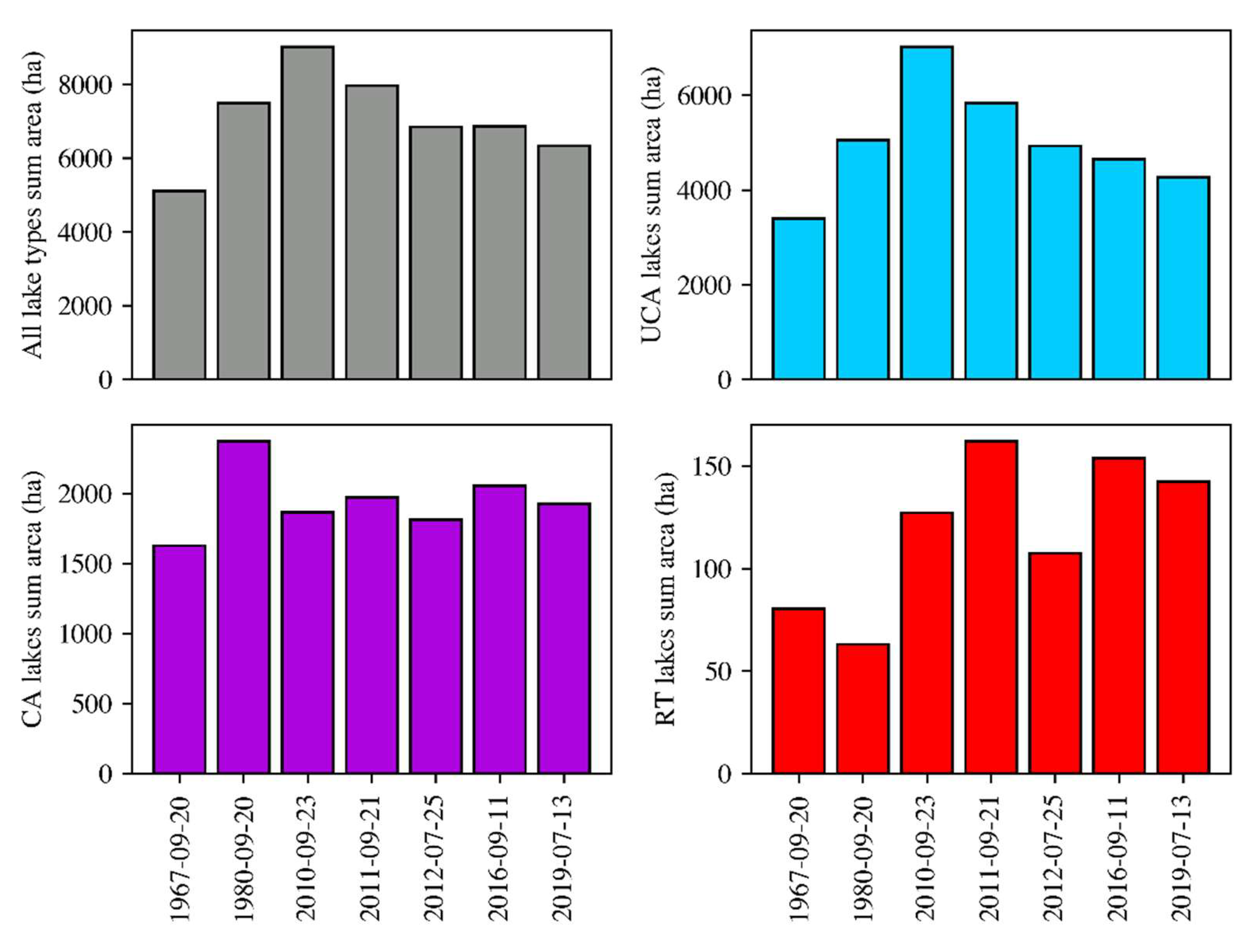
• UCA lakes appear to be particularly sensitive to increasing evapotranspiration and changes in precipitation. These lakes are hydrologically isolated, and their surface area is controlled only by evaporation and precipitation. RT lakes and CA lakes were less affected, and their lake levels are controlled by expansion into surrounding permafrost and connecting streams and rivers, respectively.
• RT lakes exhibited the strongest clustering of the three lake types. Many RT lakes formed adjacent to human disturbance (forest removal, road building, etc.). Some RT lakes, however, formed in the absence of any disturbance, likely because of climate warming. RT lake surface area is significantly positively correlated to temperature and evapotranspiration for both study sites.

References

1. Brown, J.; Ferrians, O.J., Jr.; Heginbottom, J.A.; Melnikov, E.S. Circum-Arctic Map of Permafrost and Ground-Ice Conditions; USGS: Reston, VA, USA, 1997. [Google Scholar]
2. Obu, J.; Westermann, S.; Bartsch, A.; Berdnikov, N.; Christiansen, H.H.; Dashtseren, A.; Delaloye, R.; Elberling, B.; Etzelmüller, B.; Kholodov, A.; et al. Northern Hemisphere Permafrost Map Based on TTOP Modelling for 2000–2016 at 1 km2 Scale. Earth-Sci. Rev. 2019, 193, 299–316. [Google Scholar] [CrossRef]
3. Schirrmeister, L.; Froese, D.; Tumskoy, V.; Grosse, G.; Wetterich, S. Yedoma: Late Pleistocene Ice-Rich Syngenetic Permafrost of Beringia. Encycl. Quat. Sci. 2013, 3, 542–552. [Google Scholar] [CrossRef] [Green Version]
4. Strauss, J.; Schirrmeister, L.; Grosse, G.; Fortier, D.; Hugelius, G.; Knoblauch, C.; Romanovsky, V.; Schädel, C.; Schneider von Deimling, T.; Schuur, E.A.G.; et al. Deep Yedoma Permafrost: A Synthesis of Depositional Characteristics and Carbon Vulnerability. Earth-Sci. Rev. 2017, 172, 75–86. [Google Scholar] [CrossRef] [Green Version]
5. Schuur, E.A.; McGuire, A.D.; Schädel, C.; Grosse, G.; Harden, J.W.; Hayes, D.J.; Hugelius, G.; Koven, C.D.; Kuhry, P.; Lawrence, D.M.; et al. Climate Change and the Permafrost Carbon Feedback. Nature 2015, 520, 171–179. [Google Scholar] [CrossRef]
6. Hughes-Allen, L.; Bouchard, F.; Laurion, I.; Séjourné, A.; Marlin, C.; Hatté, C.; Costard, F.; Fedorov, A.; Desyatkin, A. Seasonal Patterns in Greenhouse Gas Emissions from Thermokarst Lakes in Central Yakutia (Eastern Siberia). Limnol. Oceanogr. 2021, 66, S98–S116. [Google Scholar] [CrossRef]
7. Hugelius, G.; Strauss, J.; Zubrzycki, S.; Harden, J.W.; Schuur, E.A.G.; Ping, C.; Schirrmeister, L.; Grosse, G.; Michaelson, G.J.; Koven, C.D.; et al. Estimated Stocks of Circumpolar Permafrost Carbon with Quantified Uncertainty Ranges and Identified Data Gaps. Biogeosciences 2014, 11, 6573–6593. [Google Scholar] [CrossRef] [Green Version]
8. Park, H.; Kim, Y.; Kimball, J.S. Widespread Permafrost Vulnerability and Soil Active Layer Increases over the High Northern Latitudes Inferred from Satellite Remote Sensing and Process Model Assessments. Remote Sens. Environ. 2016, 175, 349–358. [Google Scholar] [CrossRef]
9. Nitze, I.; Grosse, G.; Jones, B.M.; Romanovsky, V.E.; Boike, J. Remote Sensing Quantifies Widespread Abundance of Permafrost Region Disturbances across the Arctic and Subarctic. Nat. Commun. 2018, 9, 5423. [Google Scholar] [CrossRef] [Green Version]
10. Nitze, I.; Grosse, G.; Jones, B.M.; Arp, C.D.; Ulrich, M.; Fedorov, A.; Veremeeva, A. Landsat-Based Trend Analysis of Lake Dynamics across Northern Permafrost Regions. Remote Sens. 2017, 9, 640. [Google Scholar] [CrossRef] [Green Version]
11. Hjort, J.; Streletskiy, D.; Doré, G.; Wu, Q.; Bjella, K.; Luoto, M. Impacts of Permafrost Degradation on Infrastructure. Nat. Rev. Earth Environ. 2022, 3, 24–38. [Google Scholar] [CrossRef]
12. Grosse, G.; Jones, B.; Arp, C. Thermokarst Lakes, Drainage, and Drained Basins. In Treatise on Geomorphology; USGS: Reston, VA, USA, 2013; pp. 326–349. ISBN 9780123747396. [Google Scholar]
13. Ulrich, M.; Matthes, H.; Schirrmeister, L.; Schütze, J.; Park, H.; Iijima, Y.; Fedorov, A.N. Differences in Behavior and Distribution of Permafrost-Related Lakes in Central Yakutia and Their Response to Climatic Drivers. Water Resour. Res. 2017, 53, 1167–1188. [Google Scholar] [CrossRef] [Green Version]
14. Serreze, M.C.; Barry, R.G. Processes and Impacts of Arctic Amplification: A Research Synthesis. Glob. Planet. Change 2011, 77, 85–96. [Google Scholar] [CrossRef]
15. Pörtner, H.-O.; Roberts, D.C.; Masson-Delmotte, V.; Zhai, P.; Tignor, M.; Poloczanska, E.; Mintenbeck, K.; Alegría, A.; Nicolai, M.; Okem, A.; et al. IPCC Special Report on the Ocean and Cryosphere in a Changing Climate; IPCC: Geneva, Switzerland, 2019. [Google Scholar]
16. Desyatkin, A.R.; Takakai, F.; Fedorov, P.P.; Nikolaeva, M.C.; Desyatkin, R.V.; Hatano, R. CH 4 Emission from Different Stages of Thermokarst Formation in Central Yakutia, East Siberia. Soil Sci. Plant Nutr. 2009, 55, 558–570. [Google Scholar] [CrossRef] [Green Version]
17. Bouchard, F.; Laurion, I.; Preskienis, V.; Fortier, D.; Xu, X.; Whiticar, M.J. Modern to Millennium-Old Greenhouse Gases Emitted from Ponds and Lakes of the Eastern Canadian Arctic (Bylot Island, Nunavut). Biogeosciences 2015, 12, 7279–7298. [Google Scholar] [CrossRef] [Green Version]
18. Prėskienis, V.; Laurion, I.; Bouchard, F.; Douglas, P.M.J.; Billett, M.F.; Fortier, D.; Xu, X. Seasonal Patterns in Greenhouse Gas Emissions from Lakes and Ponds in a High Arctic Polygonal Landscape. Limnol. Oceanogr. 2021, 66, S117–S141. [Google Scholar] [CrossRef]
19. French, H. Thermokarst Processes and Landforms. Periglac. Environ. 2017, 24, 169–192. [Google Scholar]
20. Bouchard, F.; Macdonald, L.A.; Turner, K.W.; Thienpont, J.R.; Medeiros, A.S.; Biskaborn, B.K.; Korosi, J.; Hall, R.I.; Pienitz, R.; Wolfe, B.B. Paleolimnology of Thermokarst Lakes: A Window into Permafrost Landscape Evolution. Arct. Sci. 2017, 3, 91–117. [Google Scholar] [CrossRef] [Green Version]
21. Verpoorter, C.; Kutser, T.; Seekell, D.A.; Tranvik, L.J. A Global Inventory of Lakes Based on High-Resolution Satellite Imagery. Geophys. Res. Lett. 2014, 41, 6396–6402. [Google Scholar] [CrossRef]
22. Liebner, S.; Welte, C.U. Roles of Thermokarst Lakes in a Warming World. Trends Microbiol. 2020, 28, 769–779. [Google Scholar] [CrossRef]
23. Elder, C.D.; Thompson, D.R.; Thorpe, A.K.; Chandanpurkar, H.A.; Hanke, P.J.; Hasson, N.; James, S.R.; Minsley, B.J.; Pastick, N.J.; Olefeldt, D.; et al. Characterizing Methane Emission Hotspots From Thawing Permafrost. Glob. Biogeochem. Cycles 2021, 35, e2020GB006922. [Google Scholar] [CrossRef]
24. Tarasenko, T. Interannual Variations in the Areas of Thermokarst Lakes in Central Yakutia. Water Resour. 2013, 40, 111–119. [Google Scholar] [CrossRef]
25. Boike, J.; Grau, T.; Heim, B.; Günther, F.; Langer, M.; Muster, S.; Gouttevin, I.; Lange, S. Satellite-Derived Changes in the Permafrost Landscape of Central Yakutia, 2000–2011: Wetting, Drying, and Fires. Glob. Planet. Change 2016, 139, 116–127. [Google Scholar] [CrossRef] [Green Version]
26. Travers-Smith, H.Z.; Lantz, T.C.; Fraser, R.H. Surface Water Dynamics and Rapid Lake Drainage in the Western Canadian Subarctic (1985–2020). J. Geophys. Res. Biogeosci. 2021, 126, e2021JG006445. [Google Scholar] [CrossRef]
27. Chen, Y.; Liu, A.; Cheng, X. Detection of Thermokarst Lake Drainage Events in the Northern Alaska Permafrost Region. Sci. Total Environ. 2022, 807, 150828. [Google Scholar] [CrossRef] [PubMed]
28. Bouchard, F.; Francus, P.; Pienitz, R.; Laurion, I.; Feyte, S. Subarctic Thermokarst Ponds: Investigating Recent Landscape Evolution and Sediment Dynamics in Thawed Permafrost of Northern Québec (Canada). Arct. Antarct. Alp. Res. 2014, 46, 251–271. [Google Scholar] [CrossRef] [Green Version]
29. Karlsson, J.M.; Lyon, S.W.; Destouni, G. Temporal Behavior of Lake Size-Distribution in a Thawing Permafrost Landscape in Northwestern Siberia. Remote Sens. 2014, 6, 621–636. [Google Scholar] [CrossRef] [Green Version]
30. Saito, H.; Iijima, Y.; Basharin, N.I.; Fedorov, A.N.; Kunitsky, V.V. Thermokarst Development Detected from High-Definition Topographic Data in Central Yakutia. Remote Sens. 2018, 10, 1579. [Google Scholar] [CrossRef] [Green Version]
31. Zhang, W.; Witharana, C.; Liljedahl, A.K.; Kanevskiy, M. Deep Convolutional Neural Networks for Automated Characterization of Arctic Ice-Wedge Polygons in Very High Spatial Resolution Aerial Imagery. Remote Sens. 2018, 10, 1487. [Google Scholar] [CrossRef] [Green Version]
32. Bhuiyan, M.A.; Witharana, C.; Liljedahl, A.K. Use of Very High Spatial Resolution Commercial Satellite Imagery and Deep Learning to Automatically Map Ice-Wedge Polygons across Tundra Vegetation Types. J. Imaging 2020, 6, 137. [Google Scholar] [CrossRef]
33. Yang, F.; Feng, T.; Xu, G.; Chen, Y. Applied Method for Water-Body Segmentation Based on Mask R-CNN. J. Appl. Remote Sens. 2020, 14, 14502. [Google Scholar] [CrossRef]
34. He, K.; Gkioxari, G.; Dollar, P.; Girshick, R. Mask R-CNN. IEEE Trans Pattern Anal Mach Intell. 2020, 42, 386–397. [Google Scholar] [CrossRef]
35. Fedorov, A.N.; Ivanova, R.N.; Park, H.; Hiyama, T.; Iijima, Y. Recent Air Temperature Changes in the Permafrost Landscapes of Northeastern Eurasia. Polar Sci. 2014, 8, 114–128. [Google Scholar] [CrossRef] [Green Version]
36. Gorokhov, A.N.; Fedorov, A.N. Current Trends in Climate Change in Yakutia. Geogr. Nat. Resour. 2018, 39, 153–161. [Google Scholar] [CrossRef]
37. Czerniawska, J.; Chlachula, J. Climate-Change Induced Permafrost Degradation in Yakutia, East Siberia. Arctic 2020, 73, 509–528. [Google Scholar] [CrossRef]
38. Ivanov, M.S. Cryogenic Structure of Quaternary Sediments in the Lena-Aldan Depression; Nauka: Novosibirsk, Russia, 1984. (In Russian) [Google Scholar]
39. Strauss, J.; Schirrmeister, L.; Grosse, G.; Wetterich, S.; Ulrich, M.; Herzschuh, U.; Hubberten, H.-W. The Deep Permafrost Carbon Pool of the Yedoma Region in Siberia and Alaska. Geophys. Res. Lett. 2013, 40, 6165–6170. [Google Scholar] [CrossRef] [PubMed] [Green Version]
40. Windirsch, T.; Grosse, G.; Ulrich, M.; Schirrmeister, L.; Fedorov, A.N.; Konstantinov, P.Y.; Fuchs, M.; Jongejans, L.L.; Wolter, J.; Opel, T.; et al. Organic carbon characteristics in ice-rich permafrost in alas and Yedoma deposits, central Yakutia. Sib. Biogeosciences 2020, 17, 3797–3814. [Google Scholar] [CrossRef]
41. Siewert, M.; Hanisch, J.; Weiss, N.; Kuhry, P.; Maximov, T.; Hugelius, G. Comparing Carbon Storage of Siberian Tundra and Taiga Permafrost Ecosystems at Very High Spatial Resolution. J. Geophys. Res. Biogeosciences 2015, 120, 1973–1994. [Google Scholar] [CrossRef] [Green Version]
42. Soloviev, P.A. The Cryolithozone of Northern Part of the Lena-Amga Interfluve; USSR Acad. Sci. Publ.: Moscow, Russia, 1959. [Google Scholar]
43. Ulrich, M.; Schmidt, J.; Ulrich, M.; Wetterich, S.; Rudaya, N.; Frolova, L.; Schmidt, J.; Siegert, C.; Fedorov, A.N.; Zielhofer, C. Rapid Thermokarst Evolution during the Mid- Holocene in Central Yakutia, Russia Rapid Thermokarst Evolution during the Mid-Holocene in Central Yakutia, Russia. Holocene 2017, 27, 1899–1913. [Google Scholar] [CrossRef]
44. Desyatkin, R.V. Soil Formation in Thermokarst Depression- Alases of Cryolithozone; Nauka: Novosibirsk, Russia, 2009. [Google Scholar]
45. Brouchkov, A.; Fukuda, M.; Fedorov, A.; Konstantinov, P.; Iwahana, G. Thermokarst as a Short-Term Permafrost Disturbance, Central Yakutia. Permafr. Periglac. Process. 2004, 51, 81–87. [Google Scholar] [CrossRef]
46. Crate, S.; Ulrich, M.; Habeck, J.O.; Desyatkin, A.R.; Desyatkin, R.V.; Fedorov, A.N.; Hiyama, T.; Iijima, Y.; Ksenofontov, S.; Mészáros, C.; et al. Permafrost Livelihoods: A Transdisciplinary Review and Analysis of Thermokarst-Based Systems of Indigenous Land Use. Anthropocene 2017, 18, 89–104. [Google Scholar] [CrossRef]
47. Fedorov, A.N.; Gavriliev, P.P.; Konstantinov, P.Y.; Hiyama, T.; Iijima, Y.; Iwahana, G. Estimating the Water Balance of a Thermokarst Lake in the Middle of the Lena River Basin, Eastern Siberia. Ecohydrology 2014, 7, 188–196. [Google Scholar] [CrossRef]
48. Séjourné, A.; Costard, F.; Fedorov, A.; Gargani, J.; Skorve, J.; Massé, M.; Mège, D. Evolution of the Banks of Thermokarst Lakes in Central Yakutia (Central Siberia) Due to Retrogressive Thaw Slump Activity Controlled by Insolation. Geomor-Phology 2015, 241, 31–40. [Google Scholar] [CrossRef]
49. Biskaborn, B.K.; Herzschuh, U.; Bolshiyanov, D.; Savelieva, L.; Diekmann, B. Environmental Variability in Northeastern Siberia during the Last ~13,300 Yr Inferred from Lake Diatoms and Sediment—Geochemical Parameters. Paleogeography Paleoclimatology Palaeoecol. 2012, 329–330, 22–36. [Google Scholar] [CrossRef]
50. Ulrich, M.; Matthes, H.; Schmidt, J.; Fedorov, A.; Siegert, C.; Schneider, B.; Strauss, J.; Zielhofer, C.; Iijima, Y. Holocene Thermokarst Dynamics in Central Yakutia—A Multi-Core and Robust Grain-Size Endmember Modeling Approach. Quat. Sci. Rev. 2019, 218C, 10–33. [Google Scholar] [CrossRef] [Green Version]
51. Soloviev, P.A. Thermokarst Phenomena and Land-Forms Due to Frost Heaving in Central Yakutia. Biul. Peryglacialny 1973, 23, 135–155. [Google Scholar]
52. Holloway, J.E.; Lewkowicz, A.G.; Douglas, T.A.; Li, X.; Turetsky, M.R.; Baltzer, J.L.; Jin, H. Impact of Wildfire on Perma-frost Landscapes: A Review of Recent Advances and Future Prospects. Permafr. Periglac. Process. 2020, 31, 371–382. [Google Scholar] [CrossRef]
53. Hughes-Allen, L.; Bouchard, F.; Séjourné, A.; Gandois, L. Limnological properties of lakes in Central Yakutia (Eastern Siberia) during four seasons (2018–2019). PANGAEA. 2020. Available online: https://doi.org/10.1594/PANGAEA.919907 (accessed on 1 January 2023).
54. QGIS Development Team. QGIS Geographic Information System. Open Source Geospatial Foundation Project. 2022. Available online: http://qgis.osgeo.org (accessed on 1 January 2023).
55. Paszke, A.; Gross, S.; Massa, F.; Lerer, A.; Bradbury, J.; Chanan, G.; Killeen, T.; Lin, Z.; Gimelshein, N.; Antiga, L.; et al. PyTorch: An Imperative Style, High-Performance Deep Learning Library. In Advances in Neural Information Processing Systems 32; Curran Assoicates, Inc.: Red Hoo, NY, USA, 2019; pp. 8024–8035. [Google Scholar]
56. Lin, T.-Y.; Maire, M.; Belongie, S.; Hays, J.; Perona, P.; Ramanan, D.; Dollár, P.; Zitnick, C.L. Microsoft Coco: Common Objects in Context. In Proceedings of the European Conference on Computer Vision, Zurich, Switzerland, 6–12 September 2014; Springer: Berlin/Heidelberg, Germany, 2014; pp. 740–755. [Google Scholar]
57. Kingma, D.P.; Ba, J. Adam: A Method for Stochastic Optimization. arXiv 2014, arXiv:1412.6980 2014. [Google Scholar]
58. Sammis, T.W.; Gregory, E.J.; Kallsen, C.E. Estimating Evapotranspiration with Water-Production Functions or the Blaney-Criddle Method. Trans. ASAE 1982, 25, 1656–1661. [Google Scholar] [CrossRef]
59. Bouchard, F.; Fortier, D.; Paquette, M.; Boucher, V.; Pienitz, R.; Laurion, I. Thermokarst Lake Inception and Development in Syngenetic Ice-Wedge Polygon Terrain during a Cooling Climatic Trend, Bylot Island (Nunavut), Eastern Canadian Arctic. Cryosphere 2020, 14, 2607–2627. [Google Scholar] [CrossRef]
60. Nesterova, N.V.; Makarieva, O.M.; Fedorov, A.N.; Shikhov, A.N. Geocryological Factors of Dynamics of the Thermokarst Lake Area in Central Yakutia. Earth’s Cryosph. 2021, 25, 19–29. [Google Scholar] [CrossRef]
61. Iijima, Y.; Abe, T.; Saito, H.; Ulrich, M.; Fedorov, A.N.; Basharin, N.I.; Gorokhov, A.N.; Makarov, V.S. Thermokarst Land-scape Development Detected by Multiple-Geospatial Data in Churapcha, Eastern Siberia. Front. Earth Sci. 2021, 9, 750298. [Google Scholar] [CrossRef]
62. Yu, Q.; Epstein, H.; Engstrom, R.; Shiklomanov, N.; Streletskiy, D. Land Cover and Land Use Changes in the Oil and Gas Regions of Northwestern Siberia under Changing Climatic Conditions. Environ. Res. Lett. 2015, 10, 124020. [Google Scholar] [CrossRef]
63. Abnizova, A.; Siemens, J.; Langer, M.; Boike, J. Small Ponds with Major Impact: The Relevance of Ponds and Lakes in Permafrost Landscapes to Carbon Dioxide Emissions. Glob. Biogeochem. Cycles 2012, 26. [Google Scholar] [CrossRef] [Green Version]
Figure 1. The general study area location is outlined by the black rectangle on the globe. The study area is located within the continuous permafrost zone of Eastern Siberia, about 120 km from the city of Yakutsk. The center study site is outlined in blue on the OSM standard basemap. In the center study site, the City of Borogontsy is indicated by the blue star and Syrdakh Village is indicated by the orange star. The south study site is outlined in orange. The City of Balyktakh is indicated by the gray star. The Lena River runs south to north. The Aldan River runs east to west. The base map is OpenStreetMap standard (the green color is ‘natural grassland’). Permafrost distribution map from [1].
Remotesensing 15 01226 g001
Figure 2. Distribution of lake types in a subset of the center study area: unconnected alas lakes (clear blue), connected alas lakes (magenta), and recent thermokarst lakes (red) are outlined on the 2013-07-14 Spot image. Pictures of each lake type are shown on the right, outlined in the representative colors.
Remotesensing 15 01226 g002
Figure 3. Image showing different lake boundaries. Black arrows are pointing to fuzzy boundaries. White arrows are pointing to clear boundaries.
Remotesensing 15 01226 g003
Figure 4. Image showing half-moon shaped unconnected alas lakes (left) and a circular unconnected alas lake (right).
Remotesensing 15 01226 g004
Figure 5. Graphical representation of the individual image sections. The bold black outline represents a single satellite image. The no fill squares surrounded by thin and dashed black lines are the base images. The gray fill squares are the overlap images.
Remotesensing 15 01226 g005
Figure 6. Model development workflow. In the ‘Early model’ panel, the existing PyTorch model is fine tuned twice using a subset of satellite images and manually digitized lake polygons. In the ‘Full training’ panel, the fine tuned model is used to generate lake polygons for four satellite images. All lake polygons associated with each of the four satellite images are manually corrected and used as input for a full training of the model. Three of the 50 checkpoints of the model are saved as version 1, version 2, and version 3. The dials to the right of each ✓.n represent the different neural network parameters of each version. The ‘Inference’ panel describes the process of using the model to generate lake polygons for all of the satellite images used in the study. Because the satellite images are so big, they need to be split into smaller images before they can be used as input to the model. The satellite images are split twice into base and overlap images to reduce unwanted artifacts at the edges of the small images. After running the model, one lake polygon shapefile is saved for each of the three versions for every satellite image. The three versions are combined using ensembling. All lake polygons are manually corrected before the final lake area change analysis.
Remotesensing 15 01226 g006
Figure 7. Comparison of all 50 checkpoints to the corrected shapefile of the 2013 (July 14) test scene. False positive rate = a lake polygon was predicted where no lake exists. False negative rate = no lake polygon was predicted where a lake exists. False prediction rate = sum of false positive rate and false negative rate. (‘wrt’ = with respect to).
Remotesensing 15 01226 g007
Figure 8. Comparison of the three ensembled polygon versions to the corrected shapefile of the 2013 (July 14) test scene. False positive rate = a lake polygon was predicted where no lake exists. False negative rate = no lake polygon was predicted where a lake exists. False prediction rate = sum of false positive rate and false negative rate. (‘wrt’ = with respect to).
Remotesensing 15 01226 g008
Figure 9. Deviation of mean annual temperature from 1951–1980 average since 1960. Data is from the meteorological station of Yakutsk (World Metrological Organization Index: 24959; 62.0866°N, 129.7500°E).
Remotesensing 15 01226 g009
Figure 10. Deviation of the sum of annual precipitation from 1951–1980 average since 1960. Data is from the meteorological station of Yakutsk (World Metrological Organization Index: 24959; 62.0866°N, 129.7500°E).
Remotesensing 15 01226 g010
Figure 11. Comparison of the yearly sum (mm) of evapotranspiration (calculated using the Blaney-Criddle method) and precipitation (mm) (Data is from the meteorological station of Yakutsk (World Metrological Organization Index: 24959; 62.0866°N, 129.7500°E)).
Remotesensing 15 01226 g011
Figure 12. Histograms of lake surface area for the south study site for all lake types (gray), UCA lakes (blue), CA lakes (magenta), and RT lakes (red).
Remotesensing 15 01226 g012
Figure 13. Comparison between 12 July 198925 September 2005, 2 August 2007, and 25 July 2012 images (south study site (the center of the image is 62.270N 130.651E). Two large unconnected alas lakes are outlined in blue (lakes a, b) and one connected alas lake is outlined in purple (lake c) (1989 scene). Lakes a and b changed designation to CA lakes in the 2007 scene. The inflows to the lakes are indicated by the blue squares.
Remotesensing 15 01226 g013
Figure 14. Comparison between the 12 July 1989 image, 25 September 2005 image, 2 August 2007 image and 8 September 2011 images. UCA lakes are outlined in blue. RT lakes are outlined in red. Lakes outside of the ~35 lakes discussed in the text are not outlined.
Remotesensing 15 01226 g014
Figure 15. Histograms of lake surface area for the center study site for all lake types (gray), UCA lakes (blue), CA lakes (magenta), and RT lakes (red).
Remotesensing 15 01226 g015
Figure 16. 1967 (September 20) scene (left) and 2010 (September 23) scene (right). In the 1967 scene, there are many UCA basins which have no lake or only a small residual lake. In the 2010 scene, most of these lake basins are occupied by more substantial UCA lakes.
Remotesensing 15 01226 g016