An Unsupervised Saliency-Guided Deep Convolutional Neural Network for Accurate Burn Mapping from Sentinel-1 SAR Data

Abstract

SAR data provide sufficient information for burned area detection in any weather condition, making it superior to optical data. In this study, we assess the potential of Sentinel-1 SAR images for precise forest-burned area mapping using deep convolutional neural networks (DCNN). Accurate mapping with DCNN techniques requires high quantity and quality training data. However, labeled ground truth might not be available in many cases or requires professional expertise to generate them via visual interpretation of aerial photography or field visits. To overcome this problem, we proposed an unsupervised method that derives DCNN training data from fuzzy c-means (FCM) clusters with the highest and lowest probability of being burned. Furthermore, a saliency-guided (SG) approach was deployed to reduce false detections and SAR image speckles. This method defines salient regions with a high probability of being burned. These regions are not affected by noise and can improve the model performance. The developed approach based on the SG-FCM-DCNN model was investigated to map the burned area of Rossomanno-Grottascura-Bellia, Italy. This method significantly improved the burn detection ability of non-saliency-guided models. Moreover, the proposed model achieved superior accuracy of 87.67% (i.e., more than 2% improvement) compared to other saliency-guided techniques, including SVM and DNN.

1. Introduction

Natural disasters occur every year in various regions across the globe, causing damage to the environment and human and wildlife. Wildfires are a common phenomenon in forest and grassland ecosystems. They significantly influence soil erosion and the atmosphere system, resulting in massive ecological and economic consequences [1,2,3]. Accordingly, monitoring and assessing the fires’ impacts on the natural ecosystem are necessary to plan the post-fire management of damaged areas [4,5].

Satellite remote sensing technology provides valuable information for monitoring Earth’s land covers, including burned areas caused by wildfires. Optical satellite data have been widely used to monitor and map this phenomenon [6,7,8]. Several research works have shown the potential of multispectral satellite data for fire and burned area detection and mapping. These works include large-scale wildfire monitoring and preliminary mapping with coarse spatial resolution satellite data, such as Advanced Very-High-Resolution Radiometer (AVHHR) and Moderate-Resolution Imaging Spectroradiometer (MODIS). These preliminary maps are the low-accuracy burn mapping sometimes used for the initial finding of fire locations before using other data with higher precision. Despite the low spatial resolution of these Earth observations, these sensors provide helpful information for detecting fires and burned areas with high frequency [9]. However, precise burn mapping requires finer-resolution data. Satellite data from the Landsat series and Sentinel-2 multispectral sensors were used for high-resolution burned area detection [10,11]. Integration of these two sensors leads to promising burn severity mapping results [12]. However, optical remote sensing data highly depends on weather and illumination conditions. In particular, this data’s utility might be limited in the presence of clouds.

Several studies have used Synthetic Aperture Radar (SAR) data to detect burned areas to address the limitations of optical observations. SAR sensors at various frequencies, e.g., X, C, and L, can penetrate clouds and smoke and monitor wildfires and burned areas at any time of day or night and in any weather conditions [13]. To efficiently analyze SAR data, several studies have investigated diverse methods for burned area detection, including thresholding [14], burn indices [15], and classification [5,16,17].

Classification methods have attracted increasing attention in remote sensing studies, such as decision trees [18,19], support vector machines (SVM) [20,21], hierarchical models [22], and, particularly, deep learning [23,24,25]. A large number of deep learning methods have been proposed for remote sensing applications, including multilayer perceptrons (MLPs) [26,27], autoencoders (AEs) [28,29,30], convolutional neural networks (CNNs) [31,32], graphs [33,34,35] and generative adversarial networks (GANs) [36,37]. CNNs are the most popular deep algorithm for remotely sensed image classification. They have shown great potential when combined with other models and mechanisms, such as GAN [38], graph [39,40], transformer [41], and attention mechanism [42]. CNNs and their combination with other methods have been successfully used for SAR burned area mapping [43,44].

The classification approaches are generally divided into supervised [45] and unsupervised methods [46,47]. Supervised methods typically have higher accuracy but require a reference or labeled data to train the classifier model [45]. Generating precise ground truth requires prior information and is generally performed by manual labeling, which is time-consuming and requires a lot of manual work [48]. The unsupervised methods detect changes regardless of training data with less computational cost and higher efficiency [49].

Due to the superiority of unsupervised or clustering methods in terms of efficiency and simplicity, they have gained more attention for SAR image classification. The clustering methods are usually combined with preprocessing and optimization algorithms, which lead to higher accuracy. Gong et al. [50] showed that combining fuzzy c-means (FCM) and Markov random field (MRF) techniques could reduce noise and improve classification accuracy. Similarly, combining preprocessing techniques with other methods, such as c-means [51] and wavelet transform [52], has also led to relevant results for SAR image classification.

Unsupervised saliency-guided methods have shown promising potential for unsupervised SAR data classification [53]. Zheng et al. [54] have used an unsupervised saliency-guided method and an m-means clustering to extract change regions from SAR difference images. Geng et al. [48] combined the saliency-guided method with a multilayer perceptron (MLP) deep neural network. They proposed saliency-guided deep neural networks (SGDNNs) for change detection of SAR images. In this study, they obtained a hierarchical fuzzy c-means (HFCM) clustering to select samples of the deep network.

In the case of mapping burned areas, accessing valid ground data right after the fire incident is almost impossible or requires lots of manual labeling effort. Therefore, unsupervised classification techniques provide more suitable approaches for burned area detection. Many existing novel approaches have achieved high accuracies for burned area mapping, most of which are supervised or require large datasets with high computational complexity and manual work. This study proposes a fully automated, unsupervised burned area mapping approach that can be conducted at a reasonable computational cost. The proposed framework investigates the potential of Sentinel-1 C-band SAR imagery for precise burned area mapping. It is based on an unsupervised saliency-guided fuzzy c-means deep convolutional neural network SG-FCM-DCNN. Accordingly, the difference image (DI) of the pre- and post-fire SAR data were first extracted for both VV and VH polarizations. Then, the salient regions were determined from the difference images (DI). An initial clustered image was obtained from FCM to be used as pseudo-training samples of the deep convolutional neural network (DCNN). Eventually, the burned area map was yielded as a classification result of the deep network. The primary significances of the current study are summarized as follows:

• Proposing a fully automatic framework for unsupervised burned area mapping.
• Developing a saliency-guided network for a particular case of burned area detection using Sentinel-1 C-band intensity data.
• Investigating the potential of DCNN for saliency-guided classification methods.

2. Study Areas and Data

2.1. Study Area

On 6 August 2017, a major wildfire broke out in the Rossomanno-Grottascura-Bellia regional nature reserve in the central region of Sicily, in the south of Italy [17]. Figure 1 shows a Sentinel-2 image and a map of the study area. In this event, approximately 3851 hectares of Mediterranean woodland were burned, including Eucalyptus and Mediterranean conifers.

2.2. Sentinel-1 SAR Data

The first Copernicus mission, Sentinel-1 (S1), comprises two satellites, S1-A and S1-B, that offer dual-polarization C-band SAR data with a six-day temporal resolution. The Google Earth Engine (GEE) platform was adopted to exploit the S1 level-1 ground range detected (GRD) product in interferometric wide swath (IW) mode in the present work [55]. The study area dataset is subjected to terrain correction and an advanced Lee speckle filter with a 7 × 7 window size. To reduce the amount of noise in SAR data [56]. The mean of pre- and post-fire images are acquired to reduce the noise effect further.

Table 1. Multitemporal Sentinel-1 SAR images of the study area.

Orbit	Date
Descending	24 July 2017	Pre-fire
Ascending	24 July 2017	Pre-fire
Ascending	29 July 2017	Pre-fire
Descending	30 July 2017	Pre-fire
Descending	17 August 2017	Post-fire
Ascending	17 August 2017	Post-fire
Ascending	22 August 2017	Post-fire
Descending	23 August 2017	Post-fire

shows the temporal distribution of obtained S1 data for the Rossomanno-Grottascura-Bellia fire.

2.3. Reference Data

The reference ground truth map is generated based on ΔNBR index values and visual interpretation of pre- and post-fire Sentinel-2 multispectral images. Due to its promising ability to detect burned regions, the normalized burn ratio (NBR) index is often exploited to offer reference data in similar experiments [17,56,57]. As a result, ΔNBR is determined by subtracting pre- and post-fire NBRs [7]:

NBR = (NIR − SWIR₂)/(NIR + SWIR₂)

(1)

ΔNBR = NBR_pre-fire − NBR_post-fire

(2)

where NIR and SWIR2 are the S2 near-infrared (band-8A) and short-wave infrared (band-12) bands, respectively.

3. Proposed Methodology

In this section, the analytical steps of the proposed SG-FCM-DCNN are presented. The flowchart of the main processing stages is depicted in Figure 2. As a preprocessing step, terrain correction and refined Lee were utilized to reduce the effect of noise. To further improve the quality of the Sentinel-1 SAR images, the averaged pre- and post-fire images were used. Then, the log-ratio of VV and VH polarization of pre- and post-fire images are computed. Afterward, saliency rate images are obtained using the saliency-guided technique and binarized by setting a threshold. The two binary masks are aggregated and used as a mask to remove non-salient regions from log-ratio images. These masked log-ratios and two saliency rate images are used as inputs of an initial clustering and a supervised learning technique to detect burned regions. In the initial clustering stage, FCM is used to segment input data into three categories of burned, intermediate, and unburned regions. Finally, the burned and unburned regions are used in the training stage of a supervised classification method (i.e., DCNN) to estimate the intermediate data class. Details of each of these steps are explained in the following subsections.

3.1. Log-Ratio

To extract Sentinel-1 SAR intensity features, the log-ratio index is utilized. It can be computed for both VV and VH polarizations. The most general SAR index uses the logarithm function to scale the radar burn ratio (RBR). The log-ratio is defined as follows:

log-ratio^xy = 10 log₁₀(I^XY_post-fire/I^XY_pre-fire)

(3)

where I^XY_post-fire and I^XY_pre-fire are the post-fire and pre-fire SAR intensities of XY (VV or VH) polarization, respectively.

3.2. Salient Region Detection

Salient region detection considerably reduces the impact of SAR image noises, including speckles. Salient regions represent the essential information that has the potential to change areas. Additionally, they ignore background pixels. The difference image is generally used as input for salient region detection. Here, the log-ratio is considered the suitable difference image for Sentinel-1 intensity. To generate the salient image, the log-ratio image was segmented into 27 × 27 square windows with 50% overlap. Then, the Euclidean distance (${\mathrm{d}}_{\mathrm{v}}\left({\mathrm{x}}_i,{\mathrm{x}}_j\right)$) of each window was computed using the corresponding pixel in the other window, and the center of the windows was considered to determine the geometric distance (${\mathrm{d}}_{\mathrm{p}}\left({\mathrm{x}}_i,{\mathrm{x}}_j\right)$). Then, the normalized distances were utilized to calculate the dissimilarity index between the windows [54]:

$$\mathrm{d}\left({\mathrm{x}}_i,{\mathrm{x}}_j\right)=\frac{{\mathrm{d}}_{\mathrm{v}}\left({\mathrm{x}}_i,{\mathrm{x}}_j\right)}{1+ \mathrm{C} \times { \mathrm{d}}_{\mathrm{p}}\left({\mathrm{x}}_i,{\mathrm{x}}_j\right)}$$

(4)

where C is a fixed factor balancing Euclidean and geometric distances of the windows. This factor is set to 3, which many studies recommend as the optimum value [48,53]. The window with less similarity to the others was determined as a more salient region. Computing the dissimilarity function for all windows is significantly large. To reduce the computation, only k most similar windows were considered. The k parameter is defined as k = 64, similar to other similar studies [53,54]. Accordingly, the saliency of one window compared to others is represented as follows:

$${\mathrm{S}}_{\mathrm{i}}=1\text{ – }\exp (-\frac{1}{k}\times {{\displaystyle \sum }}_{j=1}^k\mathrm{d}({\mathrm{x}}_i,{\mathrm{x}}_j))$$

(5)

To further improve the accuracy of salient point detection, various scales were used (100%, 80%, 50%, and 30%) [54]:

$${\hat{S}}_i=\frac{1}{M}{{\displaystyle \sum }}_{rϵ\mathrm{R}}^{}\left[{\mathrm{S}}_i^{\mathrm{r}}\right] (1-{\mathrm{d}}_{\mathrm{foci}}^r\left(i\right))$$

(6)

where M is the number of scales, and S^r_i and d^r_foci(i) are the saliency of ith window and geometric distance of ith window and the closest window, respectively, both at scale r. [] donates the interpolation operator to resize the map back to the original size at r scale. Eventually, the binary saliency map S is derived by setting a threshold T to the saliency image $\hat{S}$.

$$\mathrm{S}=\{\begin{array}{cc}1\hfill & \hfill \hat{S}>T\\ 0\hfill & \hfill \mathrm{o}\mathrm{t}\mathrm{h}\mathrm{e}\mathrm{r}\mathrm{w}\mathrm{i}\mathrm{s}\mathrm{e}\end{array}$$

(7)

The threshold can be obtained using an Otsu algorithm. The saliency map is then multiplied with the pre- and post-fire difference image leading to filtering background pixels. The resulting saliency images are inputs of the FCM algorithm to perform initial clustering.

3.3. Fuzzy C-Means Clustering

The filtered images are used to calculate a new difference image based on the neighborhood ratio operator with 3 × 3 windows [58]. The difference and saliency images, together with the FCM clustering method, would segment the area into M (M > 3) clusters. As changed and unchanged classes, the clusters with the highest and lowest average values were then used as training samples in the DCNN model. The rest of the clusters are considered as the test in the deep model.

3.4. Deep Convolutional Neural Network

A DCNN is used in this study to estimate an accurate burn map from the log-ratio of both VV and VH Sentinel-1 polarizations in an unsupervised saliency-guided manner. The FCM results are targets of the convolutional model. Pre- and post-fire filtered images, together with the saliency images $\hat{S}$ are inputs of the model (four layers of input features). Figure 3 shows the architecture of the used deep convolutional model. This model consists of three convolutional layers (with 32, 64, and 128 kernels of 3 by 3). Each layer hem is followed by batch normalization, max-pooling (pooling size and stride of 2), and the ReLu non-linear activation function [59]. The last convolutional layer is followed by two fully connected (FC) layers and a sigmoid activation function to produce a burn confidence map.

An L2 norm regularization with a cross-entropy loss function and a 0.5 dropout was used to reduce the overfitting impact on the deep model performance. An Adam optimizer is obtained to train the model and minimize the cost function with a learning rate of 0.001 [60]. Convolutional layers leverage convolutional kernels’ feature extraction capabilities to get low- and high-level features through various layers (from initial to deeper layers). Each convolutional layer’s output is expressed as follows:

H^l = h (w^l * H^l−1 + b^l)

(8)

The outputs of the lth and (l − 1)th layers are shown by H^l and H^l−1, and h() is the activation function. Convolutional operation is indicated by (*). Weights and bias of the lth layer are represented by w^l and b^l.

3.5. Evaluation Parameters

Four evaluation factors, including precision (P), recall (R), F1-score (F1), and overall accuracy (OA), are used to assess the effectiveness of the proposed method. These statistical parameters can be calculated based on the number of true positive (TP), true negative (TN), false positive (FP), and false negative (FN) samples:

$$\mathrm{P}=\frac{\mathrm{TP}}{\mathrm{TP}+\mathrm{FP}}$$

(9)

$$\mathrm{R}=\frac{\mathrm{TP}}{\mathrm{TP}+\mathrm{FN}}$$

(10)

$$\mathrm{F}1=\frac{2 · \mathrm{P} · \mathrm{R}}{\mathrm{P}+\mathrm{R}}$$

(11)

$$\mathrm{PA}=\frac{\mathrm{TP}+\mathrm{TN}}{\mathrm{TP}+\mathrm{TN}+\mathrm{FP} + \mathrm{FN}}$$

(12)

Precision (P) is useful to show the method’s performance in detecting burned areas, while recall (R) shows the ability of the method to identify unburned areas. Both F1 and OA indicate the overall performance of the model.

4. Results

Multiple parameters need to be accurately tuned to achieve optimum burned area mapping. These parameters are for the saliency map, clustering (FCM), and classification (DCNN). The results of each of these processing steps are presented in the following sections. Furthermore, the output of the proposed model was evaluated and compared to other state-of-the-art methods in Section 4.4.

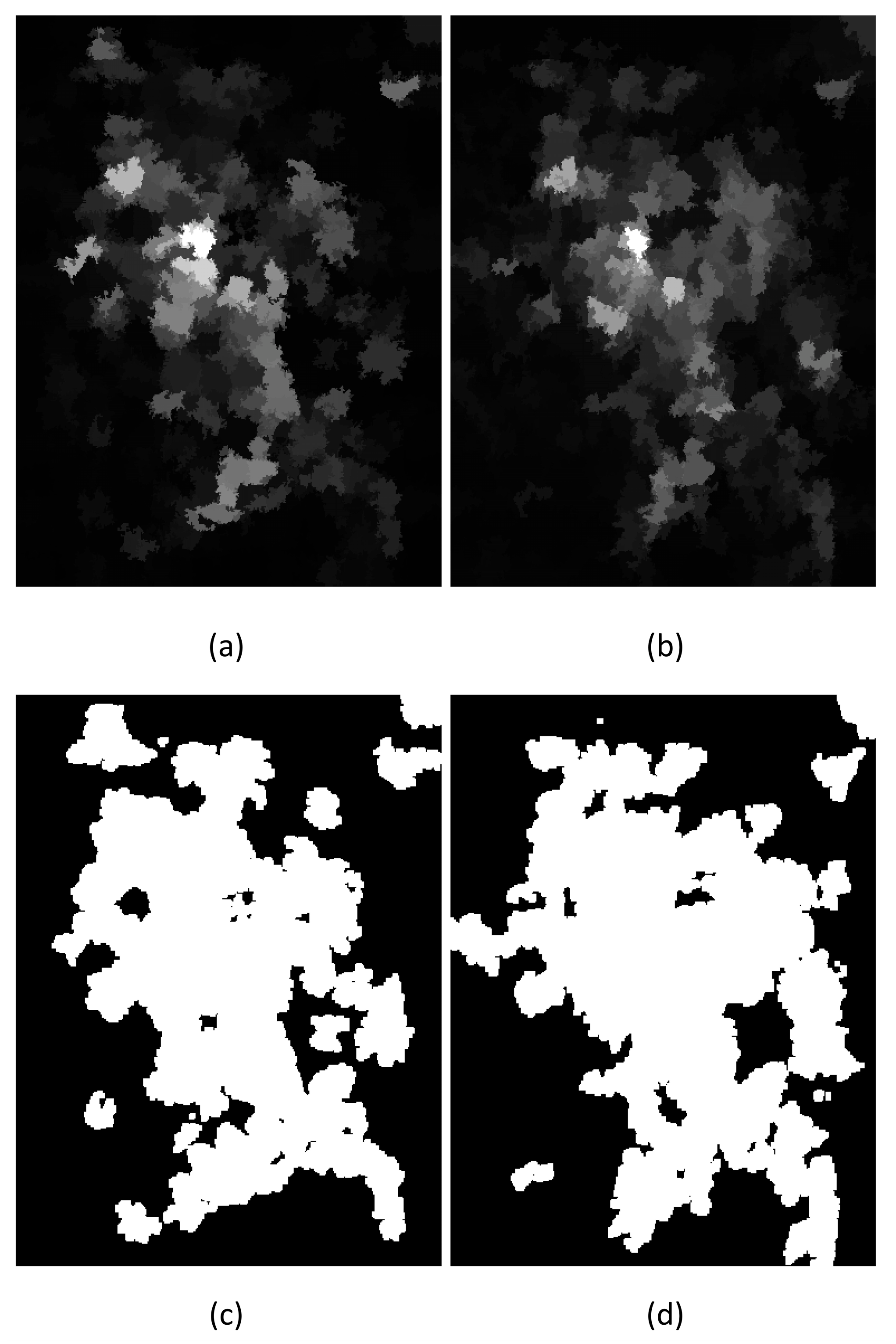
4.1. Saliency-Guided Image and Map

Saliency rate images (for each polarization) were obtained from the difference image of pre- and post-fire SAR data. Afterward, binary saliency maps were determined by setting thresholds based on the Otsu algorithm. These thresholds were set to 0.13 and 0.15 for VV and VH polarizations, respectively. The saliency rate and maps for the VV and VH polarizations are shown in Figure 4. Next, the binary saliency maps for both polarizations are aggregated. This saliency map, used in the proposed method, uses both polarizations. The detected salient regions have a higher probability of burn occurrence, which reduces background noise and false alarms.

4.2. Fuzzy C-Means Clustering

FCM clustering was applied to log-ratio and saliency images to split the data into three categories: burned, intermediate, and unburned regions. Other studies demonstrated that using more than eight clusters does not significantly improve FCM clustering results when classifying SAR data using a saliency-guided approach [48]. Accordingly, we clustered the SAR images into M = 10 classes (Figure 5). These clusters are sorted based on their probability of belonging to the burned area. The clusters with more than 80% probability of belonging to either burned or unburned classes were considered training data to be fed to the deep model (Figure 6). For the VV polarization, the classes with a high and a low probability of burned pixels were not appropriately distributed over the salient regions.

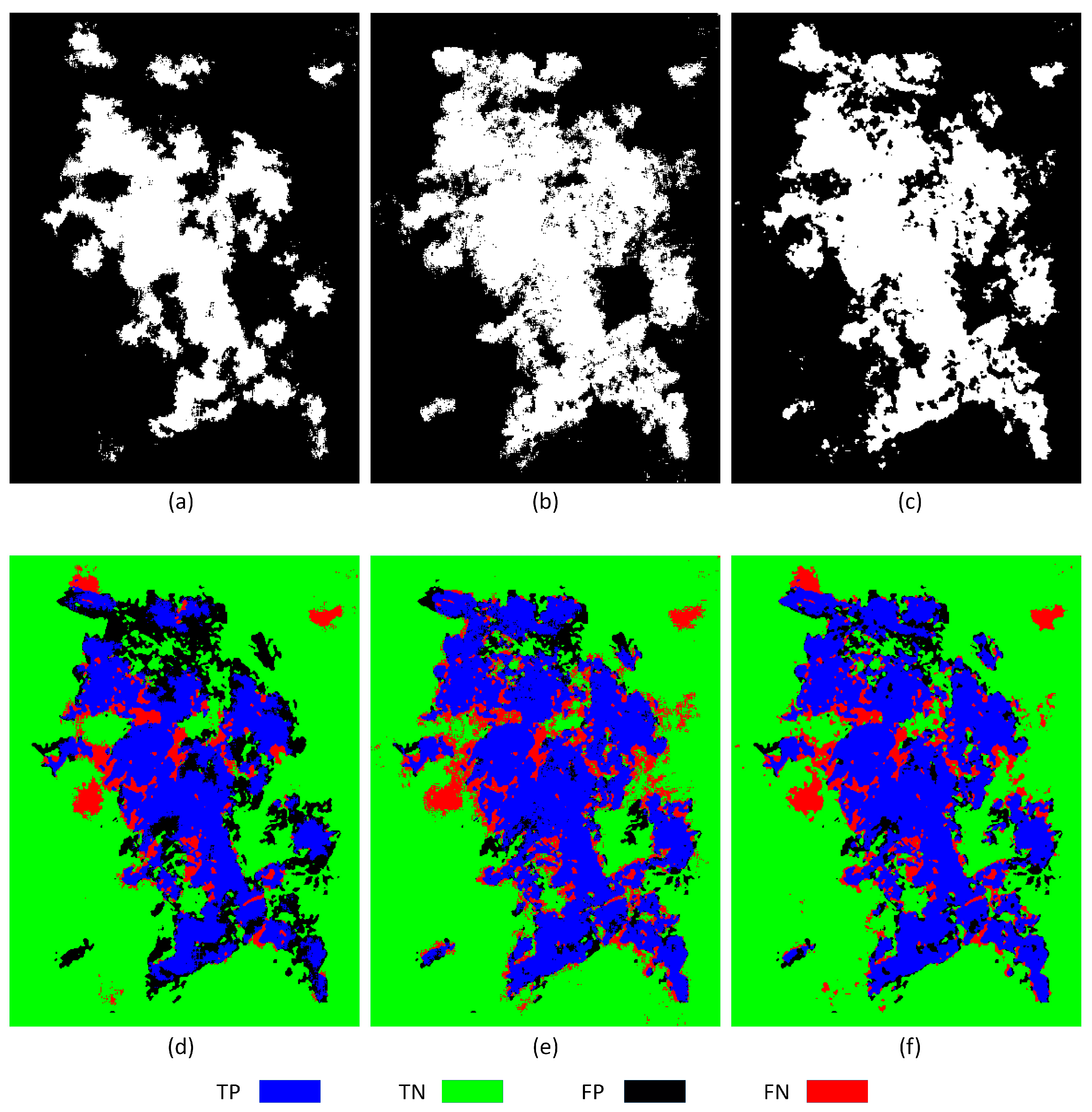
4.3. Deep Convolutional Neural Network

The log-ratio difference and saliency images (masked by binary saliency map) were the input features of the deep model. The model was then trained based on these features and the training data from the FCM results. The trained model determines whether the intermediate FCM clusters belong to burned or unburned classes. The burn maps of the saliency-guided deep convolution method for VV, VH, and their combination are presented in Figure 7. The confusion image in Figure 7d–f shows the model estimation compared to ground truth, which includes four groups of true positive (TP), true negative (TN), false positive (FP), and false negative (FN). The confusion image in Figure 7d indicates many undetected burned regions remained in VV output (FP). Figure 7e,f shows confusing images of VH and polarizations with similar performances. Meanwhile, using both polarizations has reduced false alarms (FN).

To compare the capacity of VV, VH, and their combination as inputs of the proposed SG-FCM-DCNN approach, statistical parameters, including precision (P), recall (R), F1-score (F1), and overall accuracy (OA), are calculated (

Table 2. Performance of the SG-FCM-DCNN using VV, VH, and both polarizations as the model input.

Input Polarization	P	R	F1	OA
VV	59.33%	79.67%	68.01%	82.75%
VH	84.58%	75.55%	79.81%	86.78%
Both	82.33%	78.75%	80.50%	87.67%

). It indicates the higher potential of VH compared to VV polarization using the proposed model for burned area detection. However, the VH polarization leads to a higher false alarm and lower R. In terms of the OA and F1-score, the combination of VH and VV polarizations performed superior to individual polarization.

4.4. Comparing to Other Methods

To analyze the performance of the proposed method, it is compared to some related unsupervised techniques, including FCM, FCM-DCNN, SG-FCM-SVM, and SG-FCM-DNN. FCM-DCNN is used to show the importance of the saliency-guided part of the proposed technique. FCM indicates the capability of the saliency-guided technique and the supervised model at the end of the model. Each model’s SG, FCM, and DCNN parts are similar to the proposed model. The SVM works with RBF kernel, and DNN has a similar setting as the one used in Geng et al. [48], namely three hidden layers with 150, 100, and 50 neurons. Confusion images of these techniques are compared to the proposed SG-FCM-DCNN using both polarizations as their inputs (Figure 8). Background noise false alarm is evident in models without saliency, including FCM and FCM-DCNN. The performance of the remaining models is almost similar; however, the proposed model still contains fewer false alarms (FN) compared to the SG-FCM-SVM and SG-FCM-DNN.

These methods are also compared with the proposed model precisely using statistical parameters in

Table 3. Statistical comparison of models’ performance.

Model	P	R	F1	OA
FCM	85.91%	48.75%	62.20%	67.74%
FCM-DCNN	62.33%	79.17%	69.75%	83.29%
SG-FCM-SVM	84.53%	72.34%	77.96%	85.23%
SG-FCM-DNN	84.89%	72.96%	78.47%	85.61%
SG-FCM-DCNN	82.33%	78.75%	80.50%	87.67%

. While FCM has the highest precision, it has poor performance regarding the background and contains lots of noise, reaching the lowest recall. FCM-DCNN, on the other hand, achieved the highest recall. However, this model did not detect many burned regions, which led to poor precision. The remaining models that used both the saliency-guided technique and FCM performed better. Generally, the proposed model achieved the best performance by reaching the F1-score and overall accuracy of 80.5% and 87.67%, respectively. The proposed approach has slightly lower P and R than other models. In other words, the other methods have resulted in more burned detected regions, which increases both P and false alarms (which reduces R). The proposed SG-FCM-DCNN, on the other hand, has a better balance between false alarms and burned area detection, which led to higher F1 and OA.

4.5. Efficiency Analysis

The experiments were performed on a Tesla T4 12 GB VRAM GPU and an Intel Xeon 2.2 GHz CPU with 12 GB RAM. The deep learning models (i.e., DNN and DCNN) were processed using GPU, while other processes were conducted using CPU. Each processing stage was performed 20 times; their average timeframes are presented in

Table 4. Average time for each processing stage.

Model	Processing Time (s)
Saliency-guided	114 ± 27 (for both polarizations)
Fuzzy c-means	18 ± 5
SVM	2 ± 1
DNN	21 ± 6
DCNN	65 ± 13

.

The saliency-guided model performance is the most time-consuming part, with an average of 114 s. Among the supervised stages (SVM, DNN, and DCNN), the DCNN used in the proposed approach requires the highest time for the training stage. The overall processing time for the SG-FCM- models with SVM, DNN, or DCNN as the classification step are 134, 153, and 197 s. This shows that, despite having the longest processing time, the proposed model is not noticeably more time-consuming than the other two models. Meanwhile, it can improve their performance decently.

Figure 9 displays the training process curves for the proposed approach’s DCNN model. During the training phase, the model was progressively improving. Both training and validation data losses were stabilized after almost 12 epochs, and the validation accuracy reached the maximum at approximately 87%. The gradual convergence of the model indicates its effective training procedure of the DCNN.

5. Discussion

The cross-polarization (VH) has been introduced as the dominant polarization in several studies when mapping burned areas using SAR data [5,13,16]. The current study explored the potential of both polarizations of Sentinel-1 (S1) for burned area detection. As a result, VH burn maps were superior to VV. The initial FCM clustering results (Figure 5) showed poor performance of the VV dataset that failed to detect several burned areas. Accordingly, the DCNN model (using only VV) was not fed with an efficient training dataset, which resulted in a substantial amount of undetected burned regions and low precision compared to VH. Meanwhile, the combination of VV and VH exceeds the overall performance of the single polarization. This combined data achieves a better F1 and OA by balancing the higher precision of VH and the lower false alarm rate (recall) of VV.

Sentinel-1 SAR data have been used widely and achieved high accuracy for burn area mapping. With additional SAR data such as ALOS-2, optical, and thermal remote sensing data, Abdikan et al. [61] predicted promising burn maps using the random forest (RF) classification method. Despite the simplicity of the machine learning classification model, extensive data collection and feature extraction were required. Moreover, it was performed in a supervised manner, which requires ground truth data and manual work. De Luca et al. [17] developed an unsupervised approach that helps to address the manual labeling procedure for generating ground truth.

Additionally, they only used SAR data, which applies to all weather conditions. However, significant feature extraction was performed to obtain multiple SAR indices and statistical parameters. This method cannot be used automatically and requires expert manual work. The proposed workflow in the current study attempts to overcome the limitations of the literature. In contrast to the previously mentioned studies, the present work does not require massive feature extraction because the DCNN model conducts the feature extraction automatically. Therefore, the proposed approach does not require expert knowledge for manual feature extraction. Compared to Abdikan et al.’s [61] approach, SG-FCM-DCNN can be implemented using only SAR data, making it advantageous in cloud or fire smoke. Foremost, the proposed framework is unsupervised and fully automated, allowing it to detect burned regions without requiring remote sensing expertise and user interaction

Several SAR change detection studies explored the saliency-guided (SG) method in combination with simple clustering approaches and DNN [48,53]. In the current study, the SG-FCM-DCNN architecture was developed to assess the potential of the SG approach when combined with DCNN. The convolutional kernels (in DCNN) can consider spatial characteristics of the SAR data in addition to the intensity features. Convolutional kernels’ neighborhood consideration contributes to the proposed method to reduce the impact of speckle noise on the final burn map. This ability of the kernels led to lower false alarms and approximately 6% higher recall (R) in the proposed SG-FCM-DCNN compared to the models using SG combined with DNN and SVM.

According to the processing times of each stage (Table 4), the SG method requires the longest processing time. The DCNN is more complex than the SVM and DNN and generally increases the processing time of the other SG-FCM models; however, the increased time due to using DCNN is not very significant. By minimally increasing the complexity, the proposed framework can improve overall burn mapping performance (F1 and OA) by more than 2%.

The FCM clustering approach had the lowest accuracy of all the other methods used in the comparative analysis, with a high false alarm rate and a poor recall of less than 50%. The FCM-DCNN model exceeded the FCM models, achieving the highest recall and lowest false alarm rate among all the models. Meanwhile, many burned regions remained undetected when using FCM-DCNN, which led to low precision. Although the SG-FCM-DNN model performed marginally better than the SG-FCM-SVM model, the model using SVM as the classifier is more efficient and requires considerably less processing time.

The proposed SG-FCM-DCNN showed promising potential for unsupervised burned area change detection and could be employed in image processing applications, including remote sensing, particularly for change and target detection. This framework can be beneficial, especially when the changed regions have spatial correlations (such as floods and fires). This high potential of the proposed strategy can be exploited in future studies to implement a more extensive experiment on different change detection cases and with various satellite sensors.

6. Conclusions

This paper proposed an unsupervised saliency-guided deep convolutional neural network model to detect burned areas using Sentinel-1 SAR images. To this end, salient regions with a high probability of containing burned areas are first detected. The process uses pre- and post-fire difference images to produce a saliency map for each VV and VH polarization. Another saliency map is produced to aggregate both polarizations to use the full potential of Sentinel-1 backscatter data. The obtained saliency maps and difference images are fed to an unsupervised fuzzy c-means to segment salient regions into 10 clusters. The classes with a high and low probability of belonging to burned areas are considered training data of the deep convolutional model, and the remaining regions are intermediate areas that are the test data of the model. Eventually, the DCNN model classifies intermediate pixels into burned and unburned areas. We conducted the proposed approach through a three-stage process to effectively address the impact of noise in SAR data and accurately classify burned areas. The SG-FCM-DCNN was implemented in a fully automated and unsupervised workflow, eliminating the need for manual intervention and expert knowledge. Its performance was examined by considering both Sentinel-1 polarizations to evaluate the method’s effectiveness compared to other models. The proposed model performs better when using both polarizations. Raw FCM results are significantly affected by background noise, which leads to a high rate of false alarms. A saliency-guided preprocessing stage leverages the model’s performance by reducing background noise. The saliency-guided techniques, including SG-FCM-SVM and SG-FCM-DNN, discriminated burned and unburn regions with relatively high overall accuracies (more than 85%). The investigated SG-FCM-DCNN model improves these models’ accuracies by more than 2% by using the advantage of a deep convolutional network. In addition to the high precision of the proposed method, it can be implemented unsupervised, enabling it to be used in diverse conditions when ground truth or a reliable training dataset is unavailable. Overall, the proposed methodology may have appeal for environmental monitoring, as it can be used in other contexts and demonstrates a strong capacity to minimize the need for user intervention and prior expertise.

References

1. Chuvieco, E. (Ed.) Earth Observation of Wildland Fires in Mediterranean Ecosystems; Springer: Berlin/Heidelberg, Germany, 2009; ISBN 978-3-642-01753-7. [Google Scholar]
2. Rosa, I.M.D.; Pereira, J.M.C.; Tarantola, S. Atmospheric Emissions from Vegetation Fires in Portugal (1990–2008): Estimates, Uncertainty Analysis, and Sensitivity Analysis. Atmos. Chem. Phys. 2011, 11, 2625–2640. [Google Scholar] [CrossRef] [Green Version]
3. Gitas, I.; Mitri, G.; Veraverbeke, S.; Polychronaki, A. Advances in Remote Sensing of Post-Fire Vegetation Recovery Monitoring—Review. In Remote Sensing of Biomass—Principles and Applications; Fatoyinbo, L., Ed.; InTech: Vienna, Austria, 2012; ISBN 978-953-51-0313-4. [Google Scholar]
4. Chuvieco, E.; Mouillot, F.; van der Werf, G.R.; San Miguel, J.; Tanase, M.; Koutsias, N.; García, M.; Yebra, M.; Padilla, M.; Gitas, I.; et al. Historical Background and Current Developments for Mapping Burned Area from Satellite Earth Observation. Remote Sens. Environ. 2019, 225, 45–64. [Google Scholar] [CrossRef]
5. Lasaponara, R.; Tucci, B. Identification of Burned Areas and Severity Using SAR Sentinel-1. IEEE Geosci. Remote Sens. Lett. 2019, 16, 917–921. [Google Scholar] [CrossRef]
6. Roy, D.P.; Lewis, P.E.; Justice, C.O. Burned Area Mapping Using Multi-Temporal Moderate Spatial Resolution Data—A Bi-Directional Reflectance Model-Based Expectation Approach. Remote Sens. Environ. 2002, 83, 263–286. [Google Scholar] [CrossRef]
7. Miller, J.D.; Knapp, E.E.; Key, C.H.; Skinner, C.N.; Isbell, C.J.; Creasy, R.M.; Sherlock, J.W. Calibration and Validation of the Relative Differenced Normalized Burn Ratio (RdNBR) to Three Measures of Fire Severity in the Sierra Nevada and Klamath Mountains, California, USA. Remote Sens. Environ. 2009, 113, 645–656. [Google Scholar] [CrossRef]
8. Loboda, T.V.; Hoy, E.E.; Giglio, L.; Kasischke, E.S. Mapping Burned Area in Alaska Using MODIS Data: A Data Limitations-Driven Modification to the Regional Burned Area Algorithm. Int. J. Wildland Fire 2011, 20, 487. [Google Scholar] [CrossRef]
9. Maier, S.W.; Russell-Smith, J. Measuring and Monitoring of Contemporary Fire Regimes in Australia Using Satellite Remote Sensing. In Flammable Australia: Fire Regimes, Biodiversity and Ecosystems in a Changing World; CSIRO Publishing: Collingwood, VIC, Australia, 2012; pp. 79–95. [Google Scholar]
10. Boschetti, L.; Roy, D.P.; Justice, C.O.; Humber, M.L. MODIS–Landsat Fusion for Large Area 30 m Burned Area Mapping. Remote Sens. Environ. 2015, 161, 27–42. [Google Scholar] [CrossRef]
11. Verhegghen, A.; Eva, H.; Ceccherini, G.; Achard, F.; Gond, V.; Gourlet-Fleury, S.; Cerutti, P. The Potential of Sentinel Satellites for Burnt Area Mapping and Monitoring in the Congo Basin Forests. Remote Sens. 2016, 8, 986. [Google Scholar] [CrossRef] [Green Version]
12. Quintano, C.; Fernández-Manso, A.; Fernández-Manso, O. Combination of Landsat and Sentinel-2 MSI Data for Initial Assessing of Burn Severity. Int. J. Appl. Earth Obs. Geoinf. 2018, 64, 221–225. [Google Scholar] [CrossRef]
13. Tanase, M.A.; Santoro, M.; de la Riva, J.; Prez-Cabello, F.; Le Toan, T. Sensitivity of X-, C-, and L-Band SAR Backscatter to Burn Severity in Mediterranean Pine Forests. IEEE Trans. Geosci. Remote Sens. 2010, 48, 3663–3675. [Google Scholar] [CrossRef]
14. Washaya, P.; Balz, T.; Mohamadi, B. Coherence Change-Detection with Sentinel-1 for Natural and Anthropogenic Disaster Monitoring in Urban Areas. Remote Sens. 2018, 10, 1026. [Google Scholar] [CrossRef] [Green Version]
15. Engelbrecht, J.; Theron, A.; Vhengani, L.; Kemp, J. A Simple Normalized Difference Approach to Burnt Area Mapping Using Multi-Polarisation C-Band SAR. Remote Sens. 2017, 9, 764. [Google Scholar] [CrossRef] [Green Version]
16. Imperatore, P.; Azar, R.; Calo, F.; Stroppiana, D.; Brivio, P.A.; Lanari, R.; Pepe, A. Effect of the Vegetation Fire on Backscattering: An Investigation Based on Sentinel-1 Observations. IEEE J. Sel. Top. Appl. Earth Obs. Remote Sens. 2017, 10, 4478–4492. [Google Scholar] [CrossRef]
17. De Luca, G.; Silva, J.M.N.; Modica, G. A Workflow Based on Sentinel-1 SAR Data and Open-Source Algorithms for Unsupervised Burned Area Detection in Mediterranean Ecosystems. GISci. Remote Sens. 2021, 58, 516–541. [Google Scholar] [CrossRef]
18. Khosravi, I.; Safari, A.; Homayouni, S.; McNairn, H. Enhanced Decision Tree Ensembles for Land-Cover Mapping from Fully Polarimetric SAR Data. Int. J. Remote Sens. 2017, 38, 7138–7160. [Google Scholar] [CrossRef]
19. Qi, Z.; Yeh, A.G.-O.; Li, X.; Lin, Z. A Novel Algorithm for Land Use and Land Cover Classification Using RADARSAT-2 Polarimetric SAR Data. Remote Sens. Environ. 2012, 118, 21–39. [Google Scholar] [CrossRef]
20. Zhang, L.; Zou, B.; Zhang, J.; Zhang, Y. Classification of Polarimetric SAR Image Based on Support Vector Machine Using Multiple-Component Scattering Model and Texture Features. EURASIP J. Adv. Signal Process. 2009, 2010, 1–9. [Google Scholar] [CrossRef] [Green Version]
21. Tao, C.; Chen, S.; Li, Y.; Xiao, S. PolSAR Land Cover Classification Based on Roll-Invariant and Selected Hidden Polarimetric Features in the Rotation Domain. Remote Sens. 2017, 9, 660. [Google Scholar] [CrossRef] [Green Version]
22. Chen, Z.; Lu, Z.; Gao, H.; Zhang, Y.; Zhao, J.; Hong, D.; Zhang, B. Global to Local: A Hierarchical Detection Algorithm for Hyperspectral Image Target Detection. IEEE Trans. Geosci. Remote Sens. 2022, 60, 1–15. [Google Scholar] [CrossRef]
23. Dalsasso, E.; Denis, L.; Tupin, F. SAR2SAR: A Semi-Supervised Despeckling Algorithm for SAR Images. IEEE J. Sel. Top. Appl. Earth Obs. Remote Sens. 2021, 14, 4321–4329. [Google Scholar] [CrossRef]
24. Jiang, X.; Liang, S.; He, X.; Ziegler, A.D.; Lin, P.; Pan, M.; Wang, D.; Zou, J.; Hao, D.; Mao, G.; et al. Rapid and Large-Scale Mapping of Flood Inundation via Integrating Spaceborne Synthetic Aperture Radar Imagery with Unsupervised Deep Learning. ISPRS J. Photogramm. Remote Sens. 2021, 178, 36–50. [Google Scholar] [CrossRef]
25. Xu, Y.; Sun, H.; Chen, J.; Lei, L.; Ji, K.; Kuang, G. Adversarial Self-Supervised Learning for Robust SAR Target Recognition. Remote Sens. 2021, 13, 4158. [Google Scholar] [CrossRef]
26. Wang, S.; Quan, D.; Liang, X.; Ning, M.; Guo, Y.; Jiao, L. A Deep Learning Framework for Remote Sensing Image Registration. ISPRS J. Photogramm. Remote Sens. 2018, 145, 148–164. [Google Scholar] [CrossRef]
27. Zhang, Y.; Hui, J.; Qin, Q.; Sun, Y.; Zhang, T.; Sun, H.; Li, M. Transfer-Learning-Based Approach for Leaf Chlorophyll Content Estimation of Winter Wheat from Hyperspectral Data. Remote Sens. Environ. 2021, 267, 112724. [Google Scholar] [CrossRef]
28. Shahabi, H.; Rahimzad, M.; Tavakkoli Piralilou, S.; Ghorbanzadeh, O.; Homayouni, S.; Blaschke, T.; Lim, S.; Ghamisi, P. Unsupervised Deep Learning for Landslide Detection from Multispectral Sentinel-2 Imagery. Remote Sens. 2021, 13, 4698. [Google Scholar] [CrossRef]
29. Xie, W.; Lei, J.; Fang, S.; Li, Y.; Jia, X.; Li, M. Dual Feature Extraction Network for Hyperspectral Image Analysis. Pattern Recognit. 2021, 118, 107992. [Google Scholar] [CrossRef]
30. Wei, H.; Xu, X.; Ou, N.; Zhang, X.; Dai, Y. DEANet: Dual Encoder with Attention Network for Semantic Segmentation of Remote Sensing Imagery. Remote Sens. 2021, 13, 3900. [Google Scholar] [CrossRef]
31. Zhang, X.; Pun, M.-O.; Liu, M. Semi-Supervised Multi-Temporal Deep Representation Fusion Network for Landslide Mapping from Aerial Orthophotos. Remote Sens. 2021, 13, 548. [Google Scholar] [CrossRef]
32. Tian, Y.; Dong, Y.; Yin, G. Early Labeled and Small Loss Selection Semi-Supervised Learning Method for Remote Sensing Image Scene Classification. Remote Sens. 2021, 13, 4039. [Google Scholar] [CrossRef]
33. Du, X.; Zheng, X.; Lu, X.; Doudkin, A.A. Multisource Remote Sensing Data Classification with Graph Fusion Network. IEEE Trans. Geosci. Remote Sens. 2021, 59, 10062–10072. [Google Scholar] [CrossRef]
34. Li, Z.; Huang, H.; Zhang, Z.; Pan, Y. Manifold Learning-Based Semisupervised Neural Network for Hyperspectral Image Classification. IEEE Trans. Geosci. Remote Sens. 2022, 60, 1–12. [Google Scholar] [CrossRef]
35. Ding, Y.; Zhang, Z.; Zhao, X.; Cai, W.; Yang, N.; Hu, H.; Huang, X.; Cao, Y.; Cai, W. Unsupervised Self-Correlated Learning Smoothy Enhanced Locality Preserving Graph Convolution Embedding Clustering for Hyperspectral Images. IEEE Trans. Geosci. Remote Sens. 2022, 60, 1–16. [Google Scholar] [CrossRef]
36. Ma, J.; Yu, W.; Chen, C.; Liang, P.; Guo, X.; Jiang, J. Pan-GAN: An Unsupervised Pan-Sharpening Method for Remote Sensing Image Fusion. Inf. Fusion 2020, 62, 110–120. [Google Scholar] [CrossRef]
37. Huang, A.; Shen, R.; Di, W.; Han, H. A Methodology to Reconstruct LAI Time Series Data Based on Generative Adversarial Network and Improved Savitzky-Golay Filter. Int. J. Appl. Earth Obs. Geoinf. 2021, 105, 102633. [Google Scholar] [CrossRef]
38. Ansith, S.; Bini, A.A. Land Use Classification of High Resolution Remote Sensing Images Using an Encoder Based Modified GAN Architecture. Displays 2022, 74, 102229. [Google Scholar] [CrossRef]
39. Jafarzadeh, H.; Mahdianpari, M.; Gill, E.W. Wet-GC: A Novel Multimodel Graph Convolutional Approach for Wetland Classification Using Sentinel-1 and 2 Imagery with Limited Training Samples. IEEE J. Sel. Top. Appl. Earth Obs. Remote Sens. 2022, 15, 5303–5316. [Google Scholar] [CrossRef]
40. Zhang, Z.; Ding, Y.; Zhao, X.; Siye, L.; Yang, N.; Cai, Y.; Zhan, Y. Multireceptive Field: An Adaptive Path Aggregation Graph Neural Framework for Hyperspectral Image Classification. Expert Syst. Appl. 2023, 217, 119508. [Google Scholar] [CrossRef]
41. Wang, H.; Chen, X.; Zhang, T.; Xu, Z.; Li, J. CCTNet: Coupled CNN and Transformer Network for Crop Segmentation of Remote Sensing Images. Remote Sens. 2022, 14, 1956. [Google Scholar] [CrossRef]
42. Cai, W.; Ning, X.; Zhou, G.; Bai, X.; Jiang, Y.; Li, W.; Qian, P. A Novel Hyperspectral Image Classification Model Using Bole Convolution with Three-Direction Attention Mechanism: Small Sample and Unbalanced Learning. IEEE Trans. Geosci. Remote Sens. 2023, 61, 1–17. [Google Scholar] [CrossRef]
43. Zhang, P.; Nascetti, A.; Ban, Y.; Gong, M. An Implicit Radar Convolutional Burn Index for Burnt Area Mapping with Sentinel-1 C-Band SAR Data. ISPRS J. Photogramm. Remote Sens. 2019, 158, 50–62. [Google Scholar] [CrossRef]
44. Ban, Y.; Zhang, P.; Nascetti, A.; Bevington, A.R.; Wulder, M.A. Near Real-Time Wildfire Progression Monitoring with Sentinel-1 SAR Time Series and Deep Learning. Sci. Rep. 2020, 10, 1322. [Google Scholar] [CrossRef] [PubMed] [Green Version]
45. Gao, F.; Dong, J.; Li, B.; Xu, Q.; Xie, C. Change Detection from Synthetic Aperture Radar Images Based on Neighborhood-Based Ratio and Extreme Learning Machine. J. Appl. Remote Sens. 2016, 10, 046019. [Google Scholar] [CrossRef]
46. Celik, T. Unsupervised Change Detection in Satellite Images Using Principal Component Analysis and $k$-Means clustering. IEEE Geosci. Remote Sens. Lett. 2009, 6, 772–776. [Google Scholar] [CrossRef]
47. Krinidis, S.; Chatzis, V. A Robust Fuzzy Local Information C-Means Clustering Algorithm. IEEE Trans. Image Process. 2010, 19, 1328–1337. [Google Scholar] [CrossRef] [PubMed]
48. Geng, J.; Ma, X.; Zhou, X.; Wang, H. Saliency-Guided Deep Neural Networks for SAR Image Change Detection. IEEE Trans. Geosci. Remote Sens. 2019, 57, 7365–7377. [Google Scholar] [CrossRef]
49. Shang, R.; Qi, L.; Jiao, L.; Stolkin, R.; Li, Y. Change Detection in SAR Images by Artificial Immune Multi-Objective Clustering. Eng. Appl. Artif. Intell. 2014, 31, 53–67. [Google Scholar] [CrossRef]
50. Gong, M.; Li, Y.; Jiao, L.; Jia, M.; Su, L. SAR Change Detection Based on Intensity and Texture Changes. ISPRS J. Photogramm. Remote Sens. 2014, 93, 123–135. [Google Scholar] [CrossRef]
51. Zheng, Y.; Zhang, X.; Hou, B.; Liu, G. Using Combined Difference Image and $k$ -Means Clustering for SAR Image Change Detection. IEEE Geosci. Remote Sens. Lett. 2014, 11, 691–695. [Google Scholar] [CrossRef]
52. Hou, B.; Wei, Q.; Zheng, Y.; Wang, S. Unsupervised Change Detection in SAR Image Based on Gauss-Log Ratio Image Fusion and Compressed Projection. IEEE J. Sel. Top. Appl. Earth Obs. Remote Sens. 2014, 7, 3297–3317. [Google Scholar] [CrossRef]
53. Majidi, M.; Ahmadi, S.; Shah-Hosseini, R. A Saliency-Guided Neighbourhood Ratio Model for Automatic Change Detection of SAR Images. Int. J. Remote Sens. 2020, 41, 9606–9627. [Google Scholar] [CrossRef]
54. Zheng, Y.; Jiao, L.; Liu, H.; Zhang, X.; Hou, B.; Wang, S. Unsupervised Saliency-Guided SAR Image Change Detection. Pattern Recognit. 2017, 61, 309–326. [Google Scholar] [CrossRef]
55. Gorelick, N.; Hancher, M.; Dixon, M.; Ilyushchenko, S.; Thau, D.; Moore, R. Google Earth Engine: Planetary-Scale Geospatial Analysis for Everyone. Remote Sens. Environ. 2017, 202, 18–27. [Google Scholar] [CrossRef]
56. Philipp, M.B.; Levick, S.R. Exploring the Potential of C-Band SAR in Contributing to Burn Severity Mapping in Tropical Savanna. Remote Sens. 2019, 12, 49. [Google Scholar] [CrossRef] [Green Version]
57. Donezar, U.; De Blas, T.; Larrañaga, A.; Ros, F.; Albizua, L.; Steel, A.; Broglia, M. Applicability of the MultiTemporal Coherence Approach to Sentinel-1 for the Detection and Delineation of Burnt Areas in the Context of the Copernicus Emergency Management Service. Remote Sens. 2019, 11, 2607. [Google Scholar] [CrossRef] [Green Version]
58. Gong, M.; Cao, Y.; Wu, Q. A Neighborhood-Based Ratio Approach for Change Detection in SAR Images. IEEE Geosci. Remote Sens. Lett. 2012, 9, 307–311. [Google Scholar] [CrossRef]
59. Krizhevsky, A.; Sutskever, I.; Hinton, G.E. Imagenet Classification with Deep Convolutional Neural Networks. Adv. Neural Inf. Process. Syst. 2012, 25, 84–90. [Google Scholar] [CrossRef] [Green Version]
60. Kingma, D.P.; Ba, J. Adam: A Method for Stochastic Optimization. arXiv 2014, arXiv:1412.6980. [Google Scholar] [CrossRef]
61. Abdikan, S.; Bayik, C.; Sekertekin, A.; Bektas Balcik, F.; Karimzadeh, S.; Matsuoka, M.; Balik Sanli, F. Burned Area Detection Using Multi-Sensor SAR, Optical, and Thermal Data in Mediterranean Pine Forest. Forests 2022, 13, 347. [Google Scholar] [CrossRef]
Figure 1. The study area’s location, Rossomanno-Grottascura-Bellia, is in the south of Italy (Left) and the post-fire Sentinel-2 image (Right). The RGB color composite is from NIR, red, and green pseudocolor images.
Remotesensing 15 01184 g001
Figure 2. Flowchart of the proposed saliency-guided fuzzy c-means deep convolutional neural network (SG-FCM-DCNN).
Remotesensing 15 01184 g002
Figure 3. The architecture of the used DCNN model.
Remotesensing 15 01184 g003
Figure 4. Saliency rate of (a) VV and (b) VH polarizations, and saliency map of (c) VV and (d) VH polarizations.
Remotesensing 15 01184 g004
Figure 5. FCM segmentation of salient regions into 10 clusters using (a) VV, (b) VH, and (c) both polarizations as input.
Remotesensing 15 01184 g005
Figure 6. Clusters with a high and low probability of belonging to burned areas in the salient regions for (a) VV, (b) VH, and (c) both polarizations as FCM input.
Remotesensing 15 01184 g006
Figure 7. Binary burn map of SG-FCM-DCNN using (a) VV, (b) VH, and (c) both polarizations and their corresponding confusion images at (df).
Remotesensing 15 01184 g007
Figure 8. Confusion image of (a) FCM, (b) FCM-DCNN, (c) SG-FCM-SVM, (d) SG-FCM-DNN, and (e) SG-FCM-DCNN.
Remotesensing 15 01184 g008
Figure 9. Convergence of (a) loss and (b) accuracy of DCNN stage of the proposed model.
Remotesensing 15 01184 g009