

An Integrated GNSS/MEMS Accelerometer System for Dynamic Structural Response Monitoring under Thunder Loading


Abstract
1. Introduction
2. Methodology
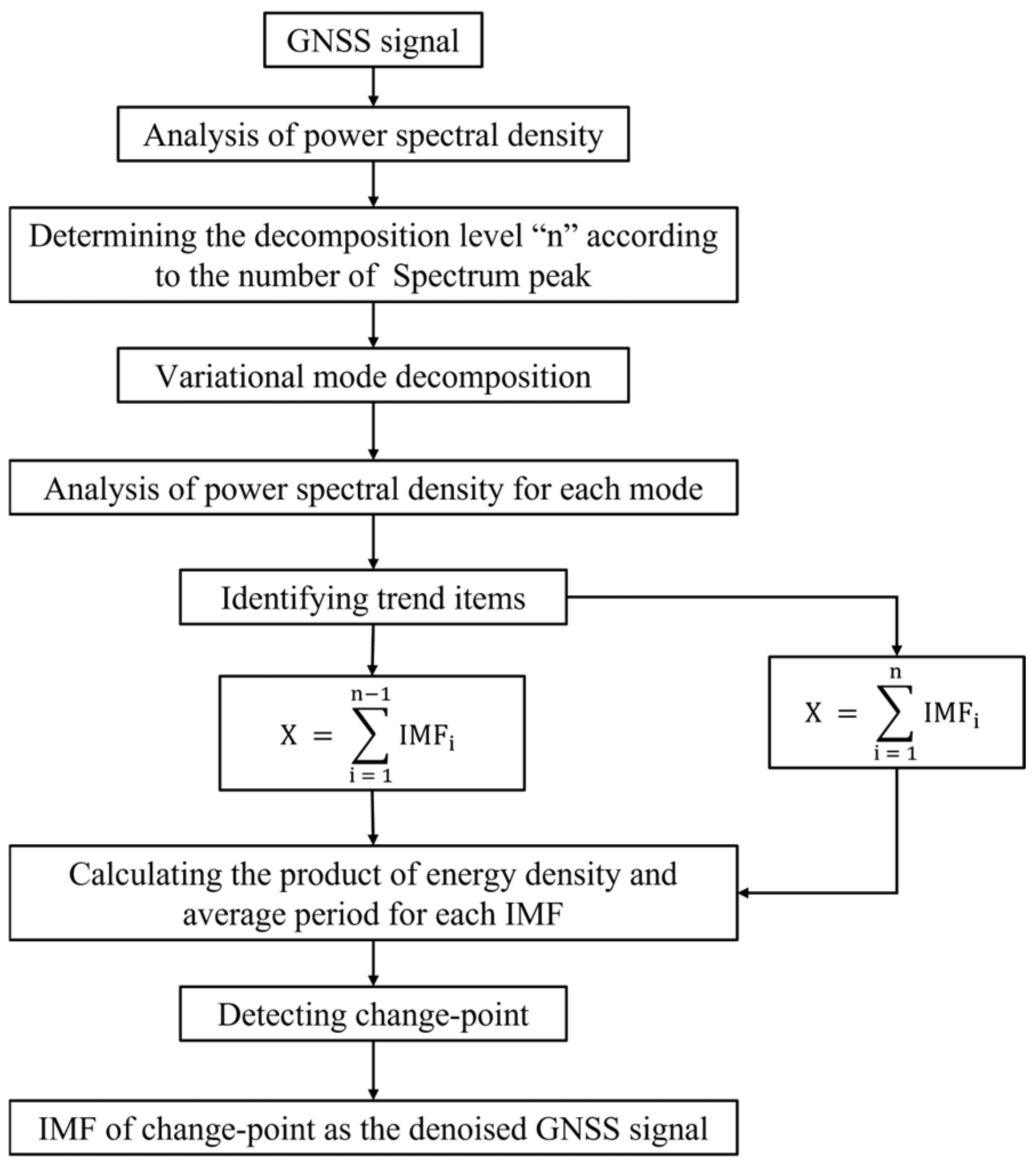
2.1. A Denoising Algorithm Combined VMD with the Characteristics of White Noise
- (1)
- Apply PSD to extract the frequency component of GNSS signals and determine the decomposition level n according to the number of spectrum peaks (the level is between five to eight empirically);
- (2)
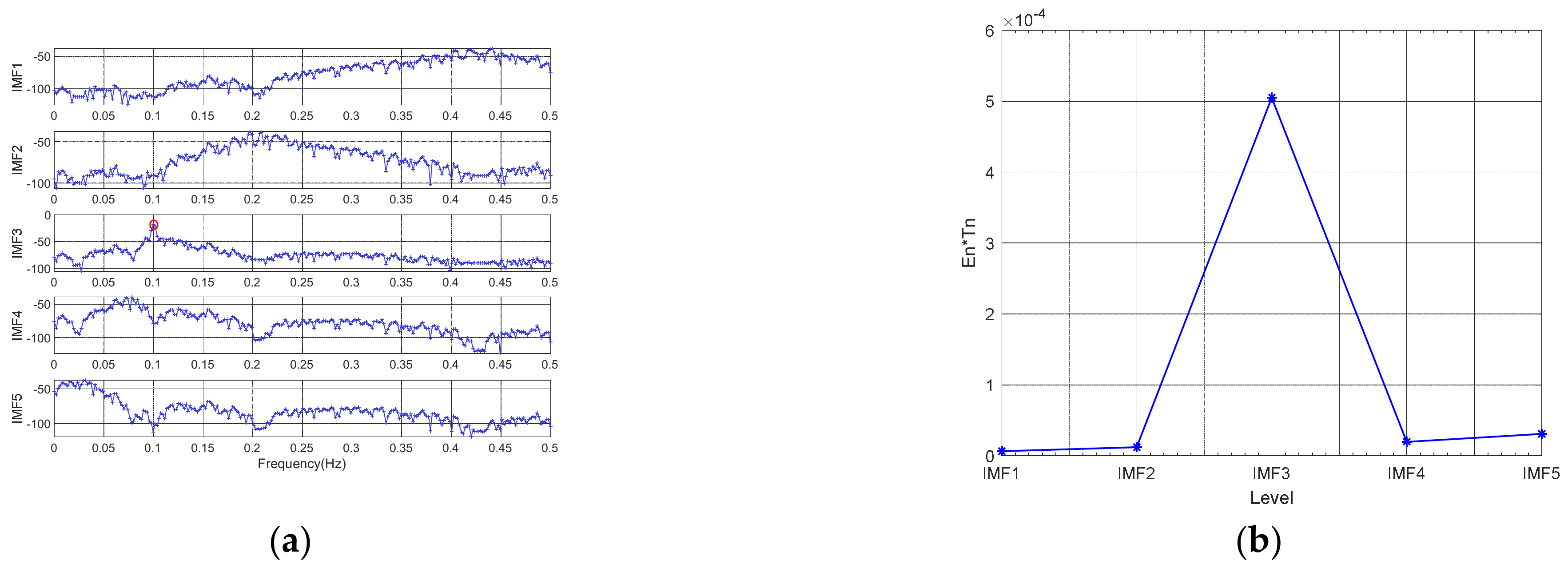
- Employ VMD to decompose the signal into different intrinsic mode functions (IMFs) from the high to low frequency bands, and extract the frequency of each IMF by PSD;
- (3)
- Check whether the signal contains a trend item based on the frequency of each IMF. If yes, the reconstructed signal is computed as follows: . Otherwise, the reconstructed signal is constructed as follows: ;
- (4)
- Calculate the product of energy density () of each IMF with Gaussian white noise and average period () of the signal;
- (5)
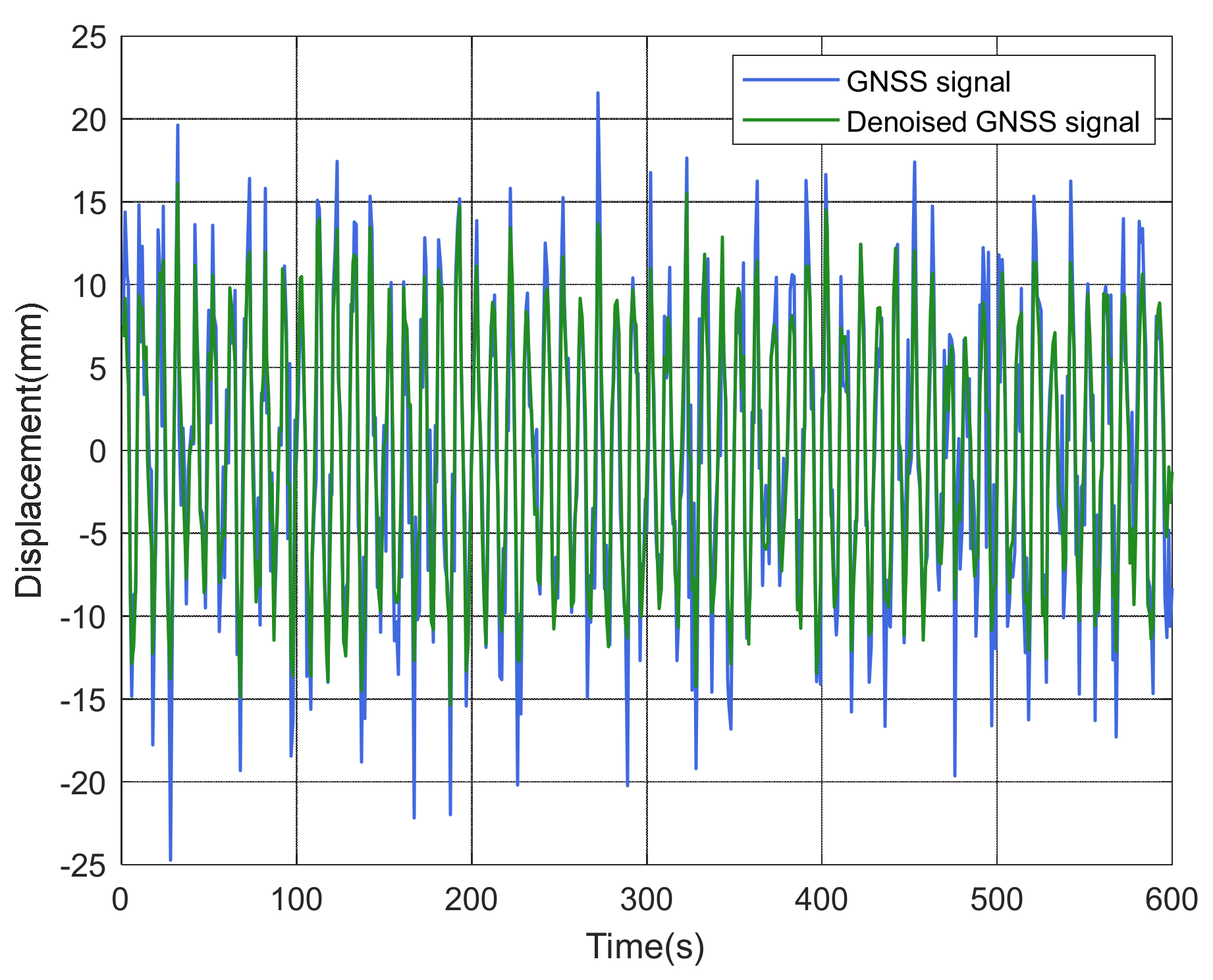
- Detect the shift points of the product as denoised signals.
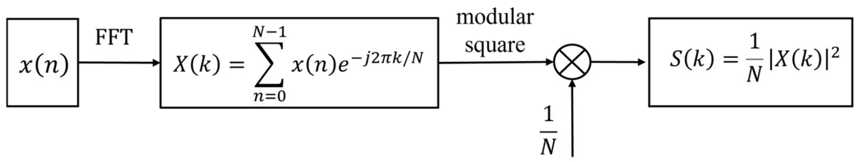
2.2. Power Spectral Density (PSD)
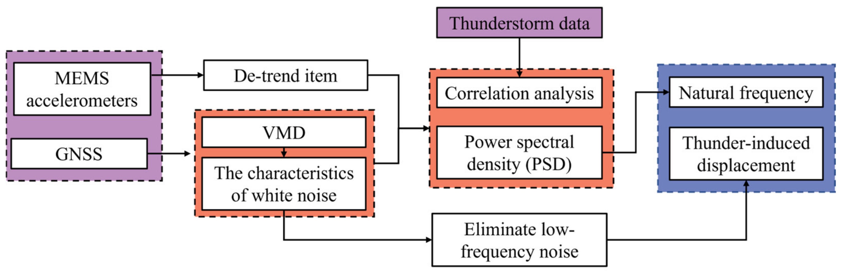
2.3. The Schematic to Detect Dynamic Responses Using an Integrated GNSS/MEMS Accelerometers System
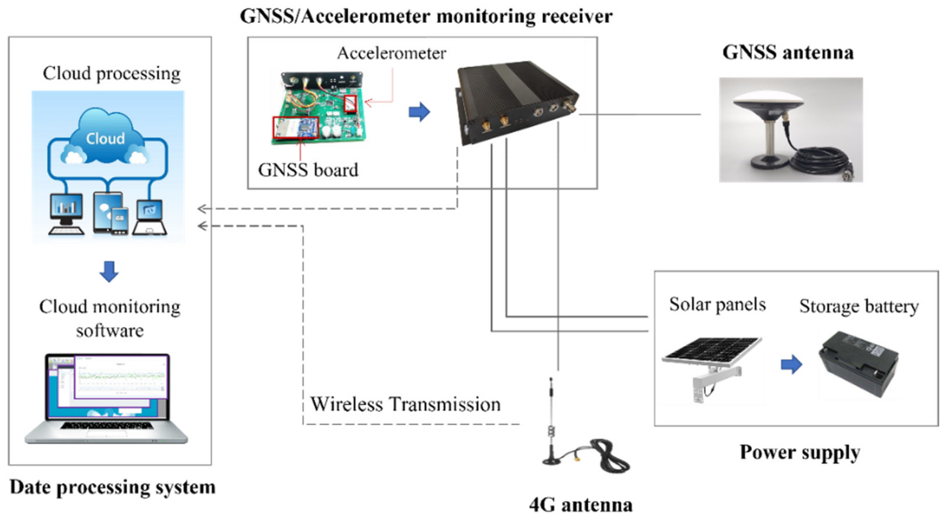
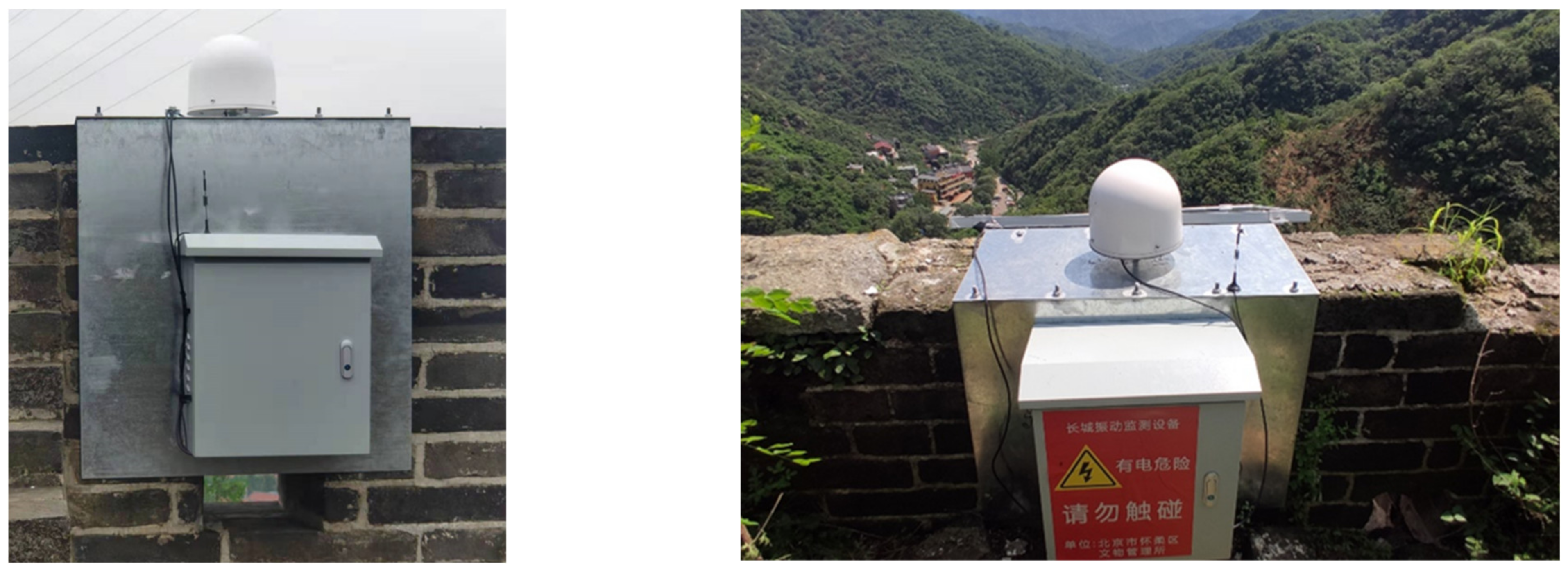
3. The GNSS/Accelerometer Vibration Monitoring System
4. Field Experiment
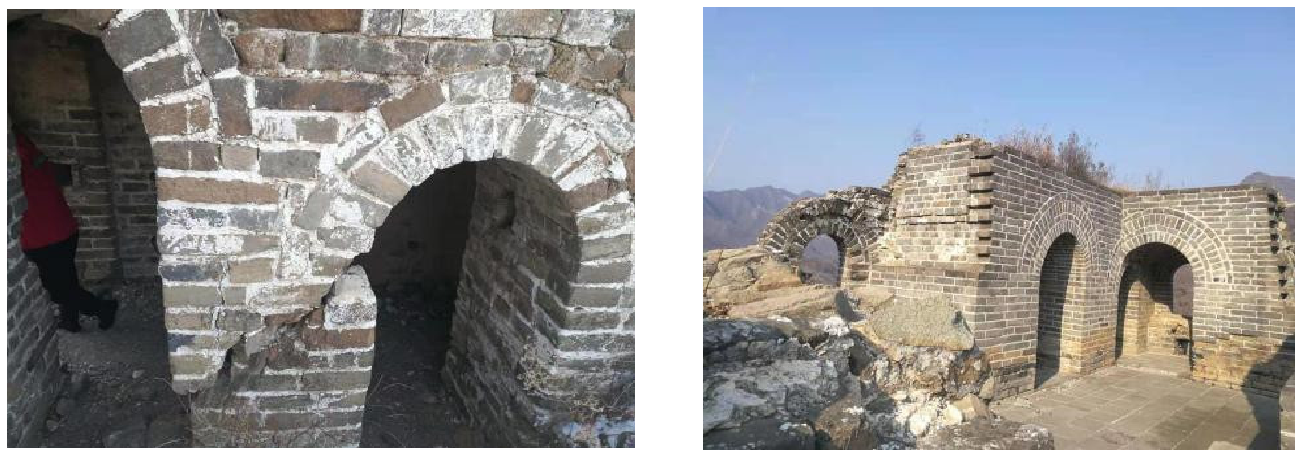
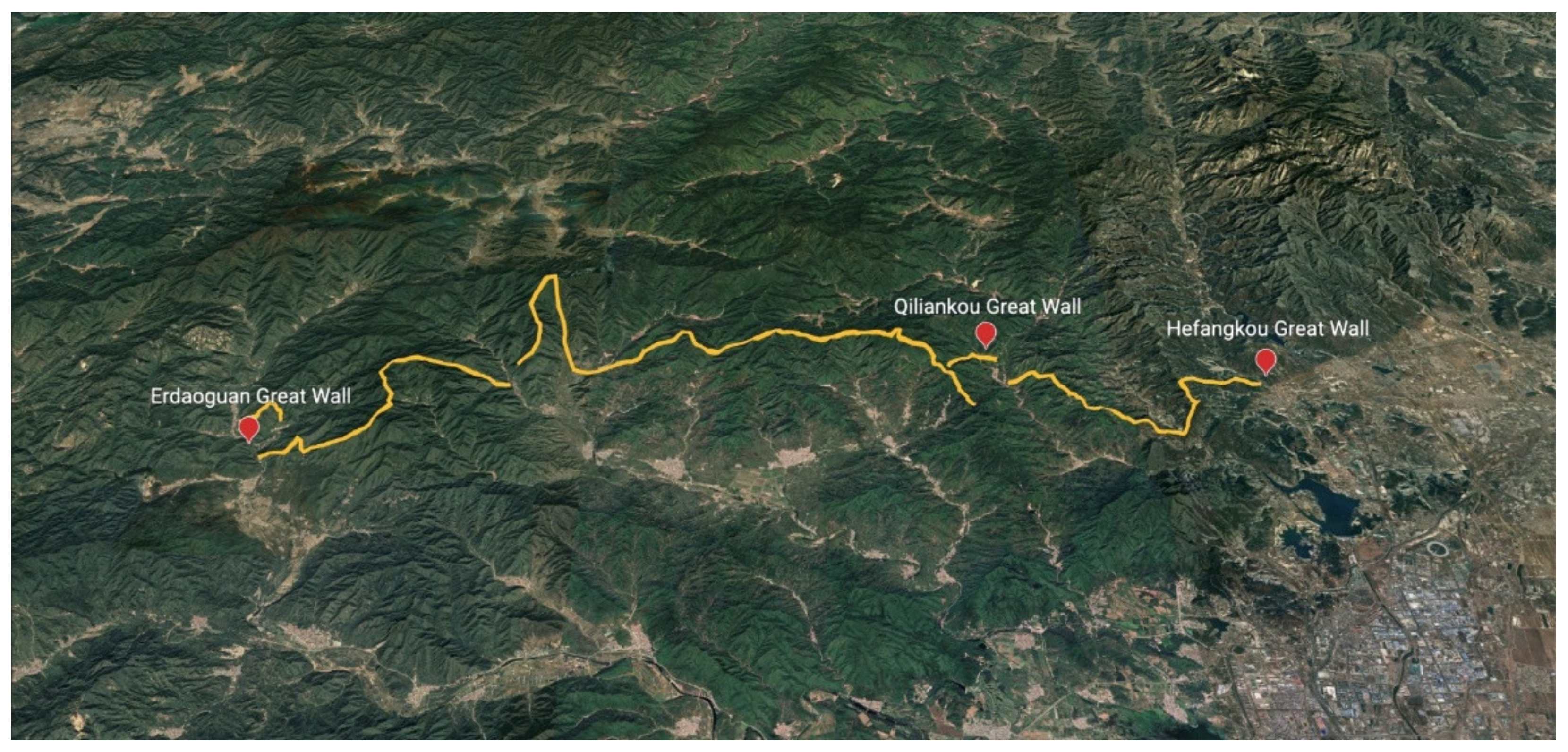
4.1. The Great Wall
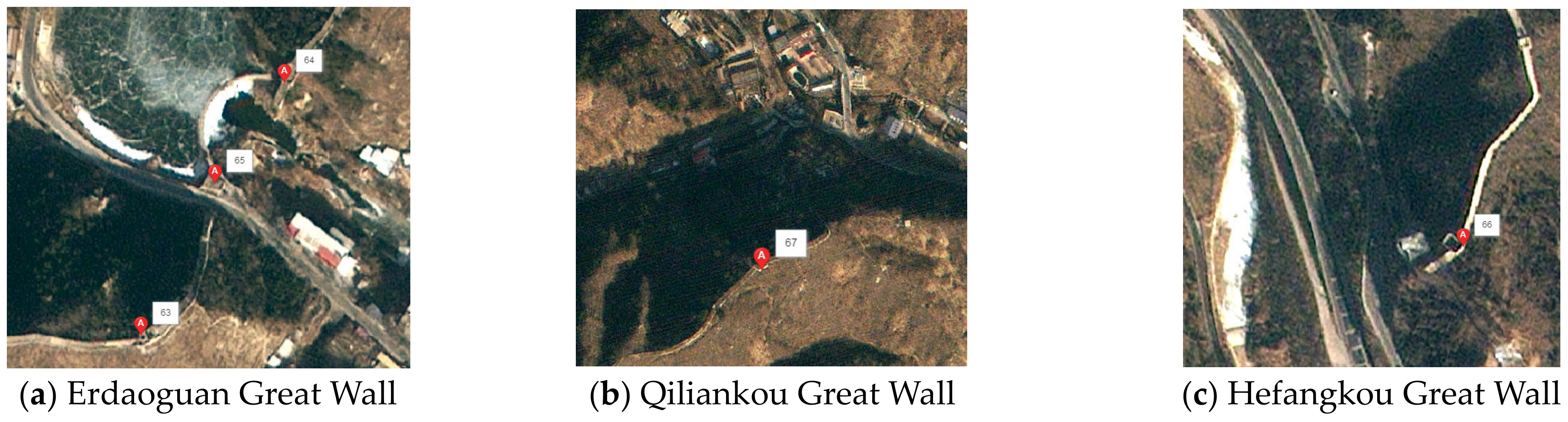
4.2. Location of the Monitoring Points
4.3. Meteorology Data
5. Results and Analysis
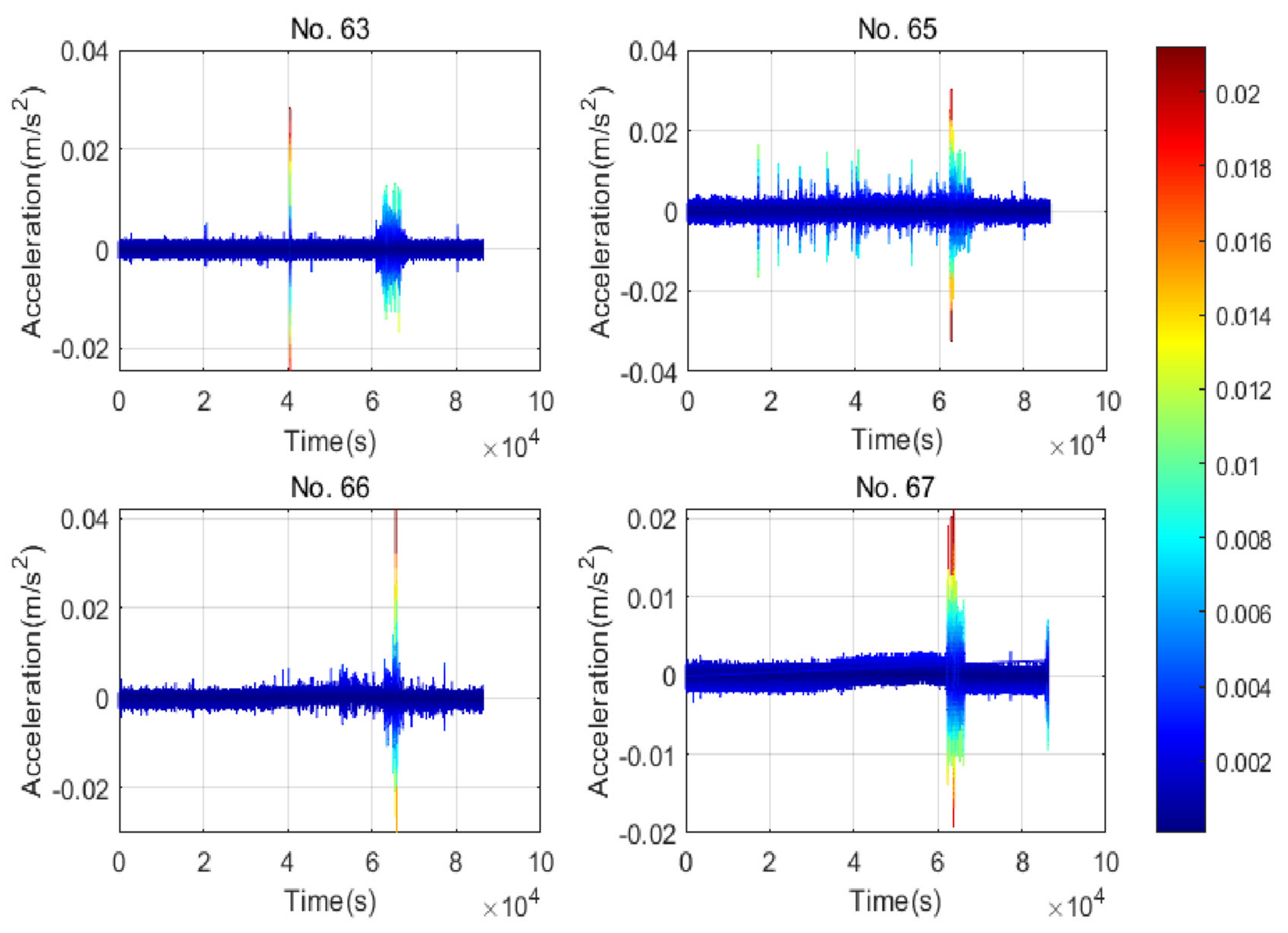
5.1. Analysis of Accelerometer Data
5.1.1. Accelerometer Data Collected on 5 July 2022
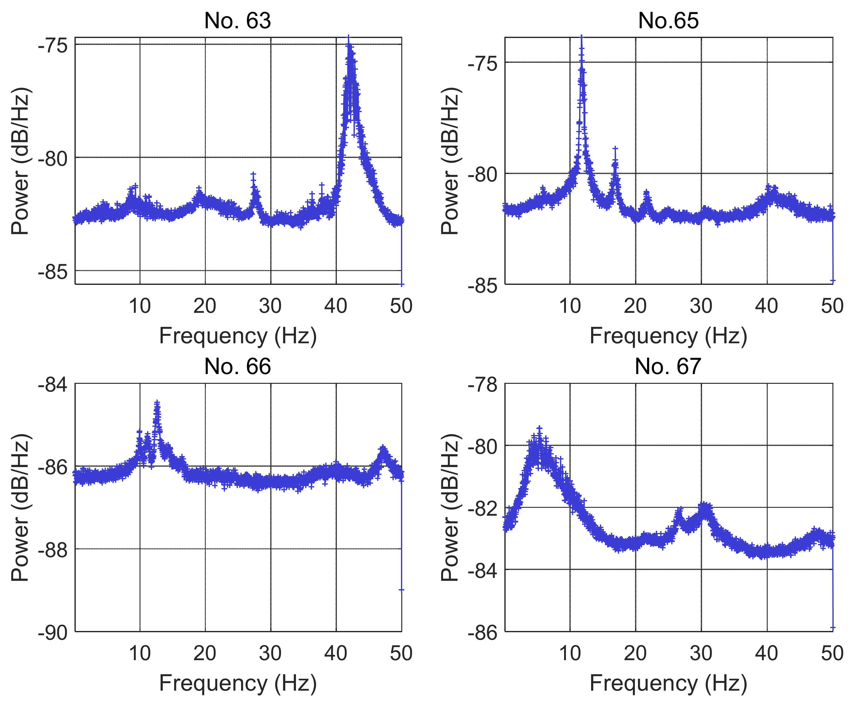
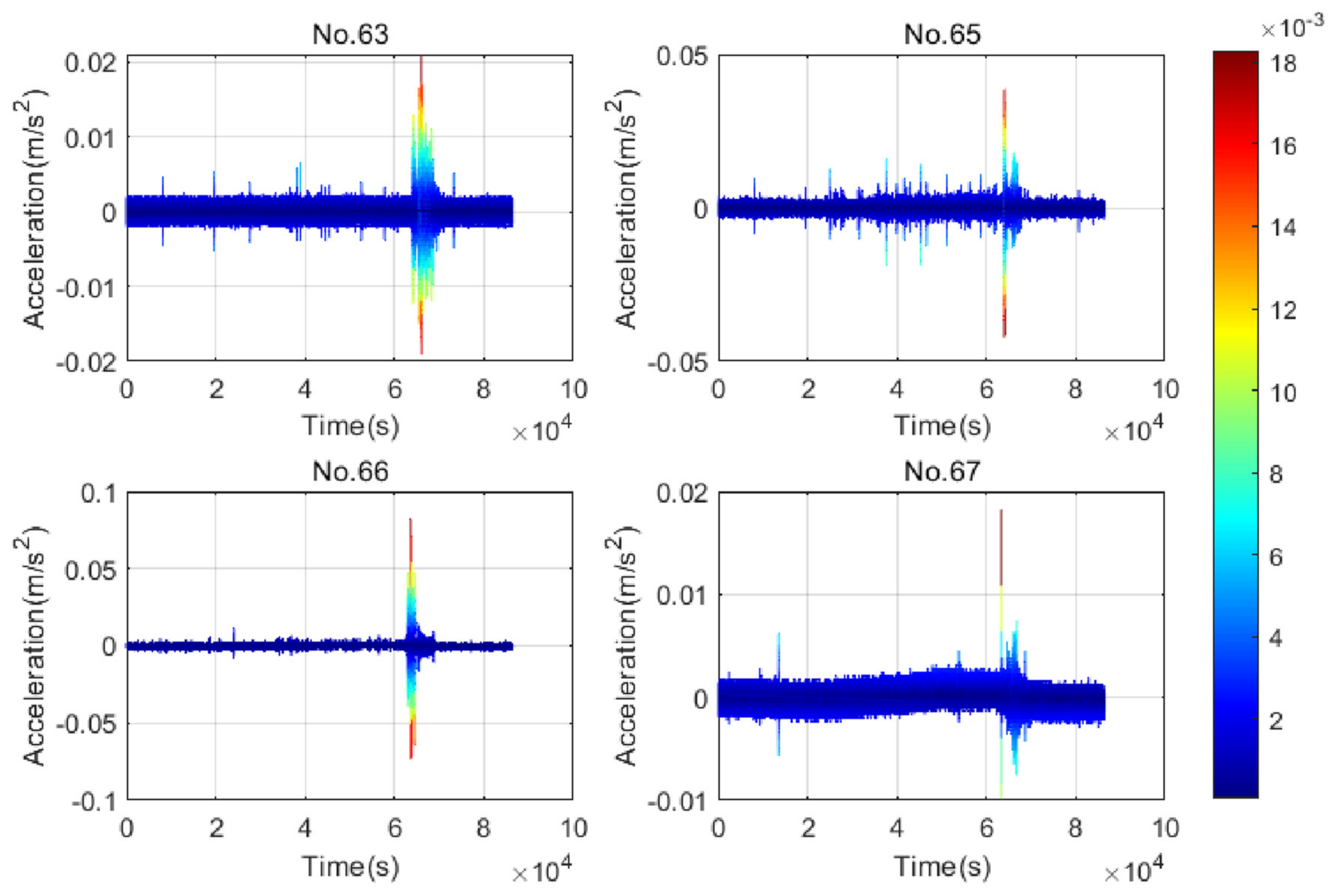
5.1.2. Accelerometer Data Collected on 4 August 2022
5.2. Analysis of GNSS Data
5.2.1. GNSS Data Collected on 5 July 2022
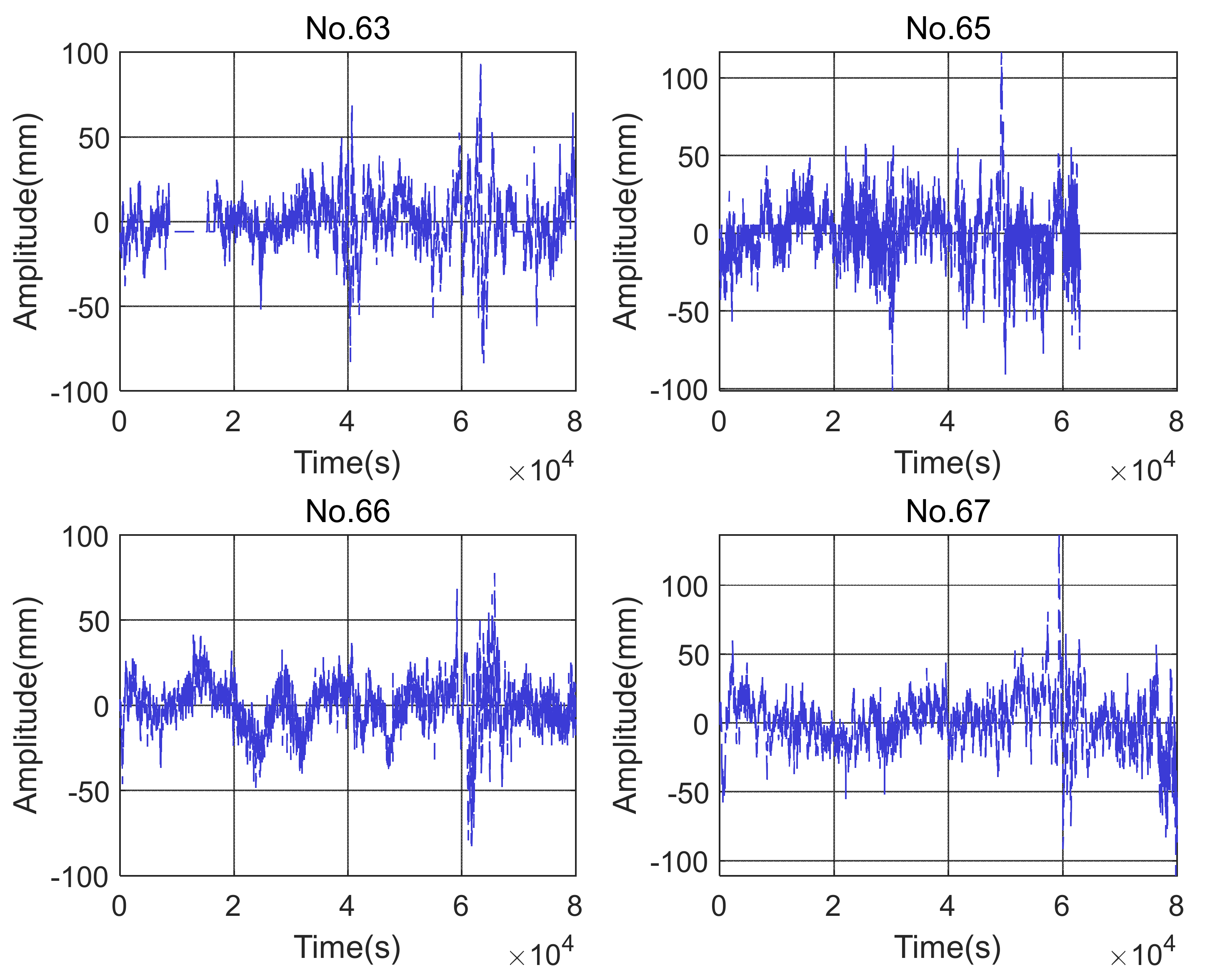
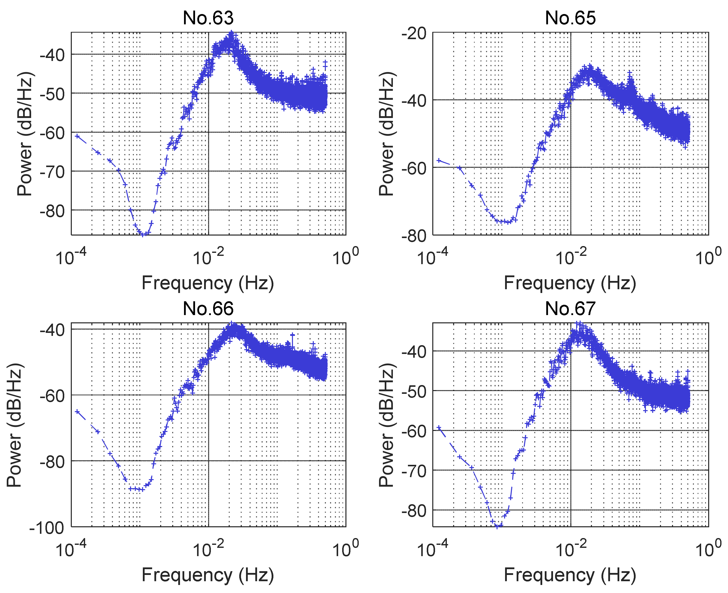
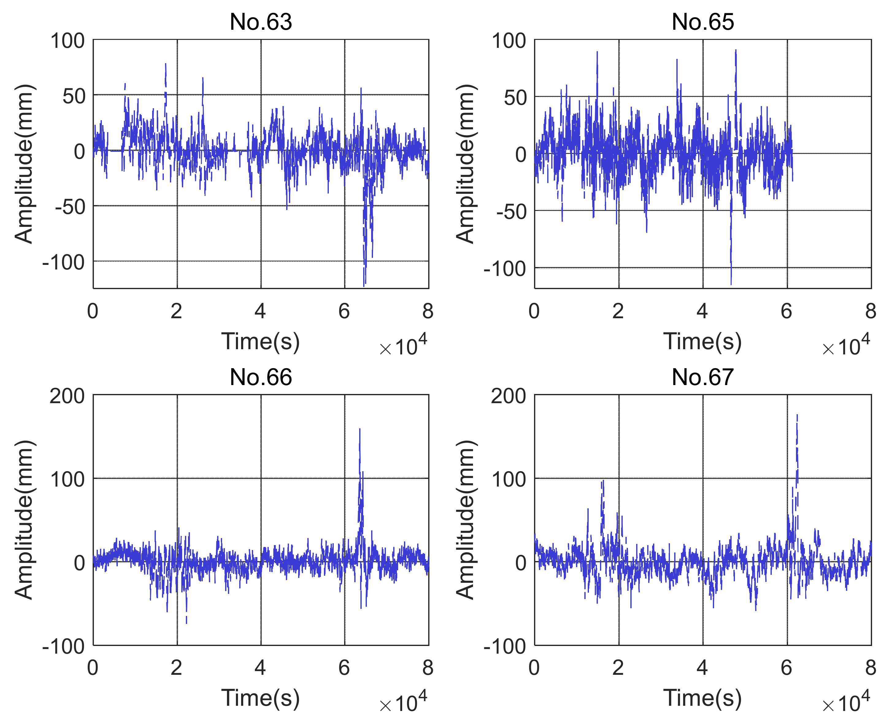
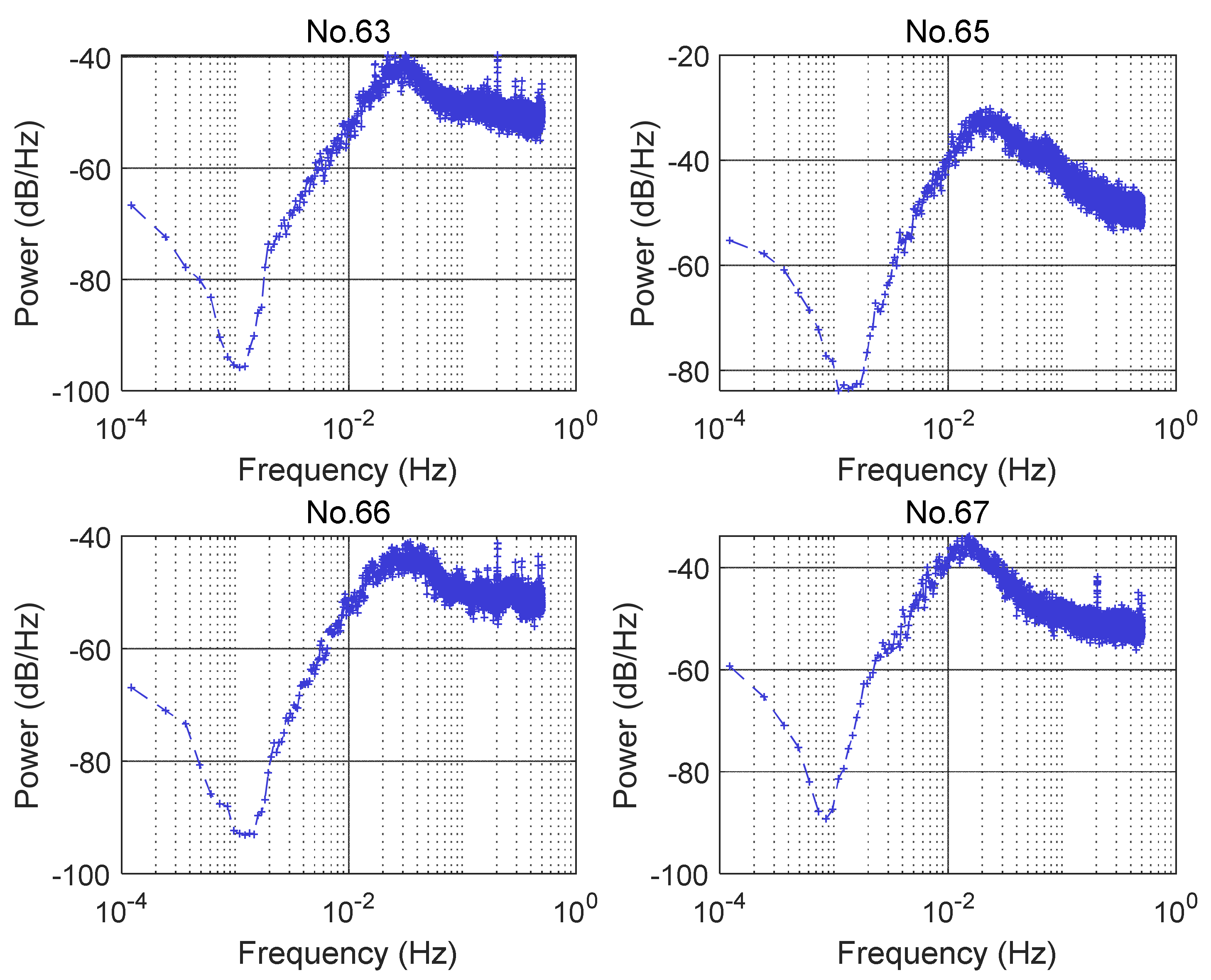
5.2.2. GNSS Data Collected on 4 August 2022
5.3. Discussion
6. Conclusions
Author Contributions
Funding
Data Availability Statement
Acknowledgments
Conflicts of Interest
References
- Shen, N.; Chen, L.; Liu, J.; Wang, L.; Tao, T.; Wu, D.; Chen, R. A Review of Global Navigation Satellite System (GNSS)-Based Dynamic Monitoring Technologies for Structural Health Monitoring. Remote Sens. 2019, 11, 1001. [Google Scholar] [CrossRef]
- Xi, R.; Jiang, W.; Meng, X.; Chen, H.; Chen, Q. Bridge monitoring using BDS-RTK and GPS-RTK techniques. Measurement 2018, 120, 128–139. [Google Scholar] [CrossRef]
- Du, H.; Chen, X.; Wang, D.K. Analysis and Evaluation of the Impact of Vehicle Driving Vibration on the Ancient Great Wall. J. Earthq. Eng. 2019, 41, 1448–1453. [Google Scholar]
- Tu, R.; Zhang, R.; Zhang, P.; Liu, J.; Lu, X. Integration of Single-Frequency GNSS and Strong-Motion Observations for Real-Time Earthquake Monitoring. Remote Sens. 2018, 10, 886. [Google Scholar] [CrossRef]
- Guerova, G.; Dimitrova, T.; Georgiev, S. Thunderstorm Classification Functions Based on Instability Indices and GNSS IWV for the Sofia Plain. Remote Sens. 2019, 11, 2988. [Google Scholar] [CrossRef]
- Qu, X.; Shu, B.; Ding, X.; Lu, Y.; Li, G.; Wang, L. Experimental Study of Accuracy of High-Rate GNSS in Context of Structural Health Monitoring. Remote Sens. 2022, 14, 4989. [Google Scholar] [CrossRef]
- Xu, P.; Shi, C.; Fang, R. High-rate precise point positioning (PPP) to measure seismic wave motions: An experimental comparison of GPS PPP with inertial measurement units. J. Geod. 2013, 87, 361–372. [Google Scholar] [CrossRef]
- Liu, X.; Wang, J.; Zhen, J.; Han, H.; Hancock, C. GNSS-aided accelerometer frequency domain integration approach to monitor structural dynamic displacements. Int. J. Image Data Fusion 2021, 12, 268–281. [Google Scholar] [CrossRef]
- Lin, J.-F.; Li, X.-Y.; Wang, J.; Wang, L.-X.; Hu, X.-X.; Liu, J.-X. Study of Building Safety Monitoring by Using Cost-Effective MEMS Accelerometers for Rapid After-Earthquake Assessment with Missing Data. Sensors 2021, 21, 7327. [Google Scholar] [CrossRef] [PubMed]
- Meng, X.; Dodson, A.H.; Roberts, G.W. Detecting bridge dynamics with GPS and triaxial accelerometers. Eng. Struct. 2007, 29, 3178–3184. [Google Scholar] [CrossRef]
- Sun, A.; Zhang, Q.; Yu, Z.; Meng, X.; Liu, X.; Zhang, Y.; Xie, Y. A Novel Slow-Growing Gross Error Detection Method for GNSS/Accelerometer Integrated Deformation Monitoring Based on State Domain Consistency Theory. Remote Sens. 2022, 14, 4758. [Google Scholar] [CrossRef]
- Li, X.; Ge, L.; Ambikairajah, E.; Rizos, C.; Tamura, Y.; Yoshida, A. Full-scale structural monitoring using an integrated GPS and accelerometer system. GPS Solut. 2006, 10, 233–247. [Google Scholar] [CrossRef]
- Meng, X.; Nguyen, D.T.; Owen, J.S.; Xie, Y.; Psimoulis, P.; Ye, G. Application of GeoSHM System in Monitoring Extreme Wind Events at the Forth Road Bridge. Remote Sens. 2019, 11, 2799. [Google Scholar] [CrossRef]
- Han, H.; Wang, J.; Meng, X.; Liu, H. Analysis of the dynamic response of a long span bridge using GPS/accelerometer/anemometer under typhoon loading. Eng. Struct. 2016, 122, 238–250. [Google Scholar] [CrossRef]
- Zeng, R.; Geng, J.; Xin, S.M. SMAG2000: Integrated GNSS strong seismograph and analysis of its seismic monitoring performance. Geomat. Inf. Sci. Wuhan Univ. 2020, 1–12. [Google Scholar] [CrossRef]
- Solari, G. Thunderstorm response spectrum technique: Theory and applications. Eng. Struct. 2016, 108, 28–46. [Google Scholar] [CrossRef]
- Roncallo, L.; Solari, G.; Muscolino, G.; Tubino, F. Maximum dynamic response of linear elastic SDOF systems based on an evolutionary spectral model for thunderstorm outflows. J. Wind. Eng. Ind. Aerodyn. 2022, 224, 104978. [Google Scholar] [CrossRef]
- Wang, Y.; Lu, G.; Shi, T.; Ma, M.; Zhu, B.; Liu, D.; Peng, C.; Wang, Y. Enhancement of Cloud-to-Ground Lightning Activity Caused by the Urban Effect: A Case Study in the Beijing Metropolitan Area. Remote Sens. 2021, 13, 1228. [Google Scholar] [CrossRef]
- Solari, G.; De Gaetano, P. Dynamic response of structures to thunderstorm outflows: Response spectrum technique vs time-domain analysis. Eng. Struct. 2018, 176, 188–207. [Google Scholar] [CrossRef]
- Dragomiretskiy, K.; Zosso, D. Variational mode decomposition. IEEE Trans. Signal Process. 2014, 62, 531–544. [Google Scholar] [CrossRef]
- Wang, J.; Liu, X.; Li, W.; Liu, F.; Hancock, C. Time–frequency extraction model based on variational mode decomposition and Hilbert–Huang transform for offshore oil platforms using MIMU data. Symmetry 2021, 13, 1443. [Google Scholar] [CrossRef]
- Flandrin, P.; Rilling, G.; Goncalves, P. Empirical mode decomposition as a filter bank. IEEE Signal Process. Lett. 2004, 11, 112–114. [Google Scholar] [CrossRef]
- Luo, Y.; Huang, C.; Zhang, J. Denoising method of deformation monitoring data based on variational mode decomposition. Geomat. Inf. Sci. Wuhan Univ. 2020, 45, 784–791. [Google Scholar]
- Yang, C.H.; Wu, T.C. Vibration measurement method of a string in transversal motion by using a PSD. Sensors 2017, 17, 1643. [Google Scholar] [CrossRef] [PubMed]
- Wang, J.; Hu, X. Application of MATLAB in Vibration Signal Processing; China Water and Power Press: Beijing, China, 2006. [Google Scholar]
- Li, Z.; Dong, Y.; Hou, M.; Wang, J.; Xin, T. Basic issues and research directions of the digital restoration of the Great Wall. Natl. Remote Sens. Bull. 2021, 25, 2365–2380. [Google Scholar]
- Available online: http://www.gov.cn/jrzg/2012-06/05/content_2153854.htm (accessed on 5 July 2022).


| Equipment | Performance | |
|---|---|---|
| GNSS | Signal tracking | BDS:B1/B2/B3; GPS: L1/L2/L5; GLONASS: L1/L2; GALILEO: E1/E5a/E5b; QZSS: L1/L5; SBAS: L1 |
| RTK(RMS) | Horizontal: ±8mm + 1 ppm; Vertical: ±15mm + 1 ppm | |
| Updating frequency | 1 Hz | |
| Accelerometer | Measurement range | 6 g |
| Noise density | 37 | |
| Offset error | 1.15 mg | |
| Linearity error | 1 mg | |
| Initial bias error (one year) | 10 mg | |
| Beijing Time | 5 July 2022 | 4 August 2022 | ||
|---|---|---|---|---|
| Weed Speed (m/s) | Severe Weather | Weed Speed (m/s) | Severe Weather | |
| 19:00 | moderate breeze (6 m/s) | moderate breeze (7 m/s) | thunderstorm | |
| 19:30 | gentle breeze (5 m/s) | (weak) thunderstorm, rain | gentle breeze (5 m/s) | (weak) thunderstorm, rain |
| 20:00 | light breeze (3 m/s) | (weak) thunderstorm, rain | light breeze (3 m/s) | (weak) thunderstorm, rain |
| 20:30 | light air (1 m/s) | (weak) thunderstorm, rain | light breeze (3 m/s) | thunderstorm, rain |
| 21:00 | light air (1 m/s) | (strong) thunderstorm | gentle breeze (4 m/s) | (weak) thunderstorm, gust, rain |
| 21:30 | light breeze (3 m/s) | light breeze (3 m/s) | thunderstorm | |
| 22:00 | light air (1 m/s) | light breeze (2 m/s | ||
| Data | 20220705 | 20220804 | ||||||
|---|---|---|---|---|---|---|---|---|
| Equipment | Accelerometer | GNSS | Accelerometer | GNSS | ||||
| Station | Max acc/ | Freq/Hz | Max amp | Freq/Hz | Max acc/ | Freq/Hz | Max amp | Freq/Hz |
| No.63 | 0.015 | 41.87 | 80 | 0.021 | 0.021 | 42.36 | 110 | 0.022 |
| No.65 | 0.041 | 11.74 | 140 | 0.019 | 0.017 | 14.11 | 120 | 0.019 |
| No.66 | 0.021 | 12.62 | 90 | 0.016 | 0.081 | 12.54 | 180 | 0.016 |
| No.67 | 0.032 | 5.35 | 110 | 0.014 | 0.041 | 6.57 | 160 | 0.014 |
| Mean | 0.027 | / | 105 | / | 0.040 | 143 | ||
Disclaimer/Publisher’s Note: The statements, opinions and data contained in all publications are solely those of the individual author(s) and contributor(s) and not of MDPI and/or the editor(s). MDPI and/or the editor(s) disclaim responsibility for any injury to people or property resulting from any ideas, methods, instructions or products referred to in the content. |
© 2023 by the authors. Licensee MDPI, Basel, Switzerland. This article is an open access article distributed under the terms and conditions of the Creative Commons Attribution (CC BY) license (https://creativecommons.org/licenses/by/4.0/).
Share and Cite
Wang, J.; Liu, X.; Liu, F.; Chen, C.; Tang, Y. An Integrated GNSS/MEMS Accelerometer System for Dynamic Structural Response Monitoring under Thunder Loading. Remote Sens. 2023, 15, 1166. https://doi.org/10.3390/rs15041166
Wang J, Liu X, Liu F, Chen C, Tang Y. An Integrated GNSS/MEMS Accelerometer System for Dynamic Structural Response Monitoring under Thunder Loading. Remote Sensing. 2023; 15(4):1166. https://doi.org/10.3390/rs15041166
Chicago/Turabian StyleWang, Jian, Xu Liu, Fei Liu, Cai Chen, and Yuyang Tang. 2023. "An Integrated GNSS/MEMS Accelerometer System for Dynamic Structural Response Monitoring under Thunder Loading" Remote Sensing 15, no. 4: 1166. https://doi.org/10.3390/rs15041166
APA StyleWang, J., Liu, X., Liu, F., Chen, C., & Tang, Y. (2023). An Integrated GNSS/MEMS Accelerometer System for Dynamic Structural Response Monitoring under Thunder Loading. Remote Sensing, 15(4), 1166. https://doi.org/10.3390/rs15041166