Urban Area Characterization and Structure Analysis: A Combined Data-Driven Approach by Remote Sensing Information and Spatial–Temporal Wireless Data

Abstract

Analysis of urban area function is crucial for urban development. Urban area function features can help to conduct better urban planning and transportation planning. With development of urbanization, urban area function becomes complex. In order to accurately extract function features, researchers have proposed multisource data mining methods that combine urban remote sensing and other data. Therefore, the research of efficient multisource data analysis tools has become a new hot topic. In this paper, a novel urban data analysis method combining spatiotemporal wireless network data and remote sensing data was proposed. First, a Voronoi-diagram-based method was used to divide the urban remote sensing images into zones. Second, we combined period and trend components of wireless network traffic data to mine urban function structure. Third, for multisource supported urban simulation, we designed a novel spatiotemporal city computing method combining graph attention network (GAT) and gated recurrent unit (GRU) to analyze spatiotemporal urban data. The final results prove that our method performs better than other commonly used methods. In addition, we calculated the commuting index of each zone by wireless network data. Combined with the urban simulation conducted in this paper, the dynamic changes of urban area features can be sensed in advance for a better sustainable urban development.

1. Introduction

Urbanization has led to a large number of people gathering in cities, and cities are environments in which people work, study, and live. Additionally, in the process of urbanization, the functions provided by urban areas became complex, which raises challenges for urban area functions analysis. The complexity [1,2,3] of urban area function is reflected in the following ways. First, the basic unit of urban activity is people. People in an area assemble into communities. The difference among crowd behaviors of communities leads to functional heterogeneity of urban areas [4,5], and, as urbanization progresses deeper, the migration and mobility of people among areas lead to dynamic changes in area function [6]. Secondly, there is heterogeneity in geographical environment among areas, such as topography [7], vegetation coverage [8], and building density and type [9]. However, area functions play a crucial role in sustainable urban development [10]. Therefore, in recent years, the characterization of urban function areas has become a hot research topic.

Traditional urban function features analysis is mainly based on survey statistics or expert judgments [11], in which main data involved are topographic maps, building-permit data [12], land use maps, and administrative boundary maps. This method relies on expert experience and survey results, so its effectiveness is limited by many subjective factors [13]. In recent years, with the rise of big data research, studies on urban function feature analysis have increasingly turned to data-driven approaches, and, from the perspective of data, urban remote sensing data is the main data source utilized for urban study [14,15,16]. For example, Zhou [17] proposed a function feature recognition method based on convolutional neural network (CNN) for urban area. The method first classified very-high-resolution (VHR) remote sensing images into basic function areas based on geographic information. Then, a trained CNN model was used to extract area function features. Ref. [18] applied remote sensing nighttime light for function characterization of urban area. This article proposed that intense night lighting is highly correlated with commercial (or industrial) areas. Conversely, areas of low light intensity are more likely to be residential. In addition to articles [17,18], many studies [19,20,21] have worked on the application of urban remote sensing data to urban function characterization, and good results have been achieved. However, as the process of urbanization deepens, functions assumed by urban areas change from singular to multiple. This complex urban system raises new challenges in the method of characterizing urban areas using only remote sensing data [22]. Facing this challenge, researchers proposed data fusion methods [23].

Urban areas are complex systems that involve both human activities and geographic environments. Human activities have a significant impact on the functions of urban areas [24]. Remote sensing data lack information on human activities [25], so the above methods cannot comprehensively analyze the functions of complex urban areas. To overcome this shortcoming, spatiotemporal data analysis was added to urban studies on the basis of urban remote sensing data [26]. The commonly used spatiotemporal data are location-based social perception data [27]. Ref. [28] proposed a hierarchical semantic recognition approach that maps urban zone by remote sensing images and point of interest (POI) data. Ref. [29] designed a new architecture to integrate remote sensing images and POI data for analyzing urban area function and provided open-source data for other researchers. POI data can reflect characteristics of human activities; however, it cannot directly provide information on the scale of human activities [30,31]. The rapid development of telecommunications and mobile technology in the past decade has fundamentally changed human activities. Therefore, researchers tend to analyze the scale of human activities by location-based cell phone data [32,33]. Ref. [34] extracted features of multiple source data which include remote sensing images and cell phone positioning data. Function features analysis of urban areas was conducted through cross-correlations. Ref. [35] first utilized cell phone signal data to extract temporal feature of human activities. Then, remote sensing images were combined for area feature identification in Changchun, China. However, most current spatiotemporal data used in urban studies were human features, which rely on expert experience and are laborious [23]. This problem was alleviated through the emergence of social media and smartphones [36]. However, location-based cell phone data raised the issue of user data privacy protection [37,38].

In this paper, in order to accurately extract function features of urban areas without using private information involving the user’s location, we adopted base-station-level wireless network traffic data. Since they reflect the crowd behavior of users served by a base station (BS), user privacy is not involved [39,40]. Wireless network data represent function features of urban area at a temporal scale; on the other hand, BS location data combined with remote sensing images provide the possibility to analyze function features of urban areas at a spatial scale. Further, we analyze causal relationships [41,42] among different urban zones and model urban function structure as causal directed graphs. The graphs reflect cross-zone movement features of human activities and provide valuable information for urban simulation. In summary, the contributions of this paper can be summarized as follows:

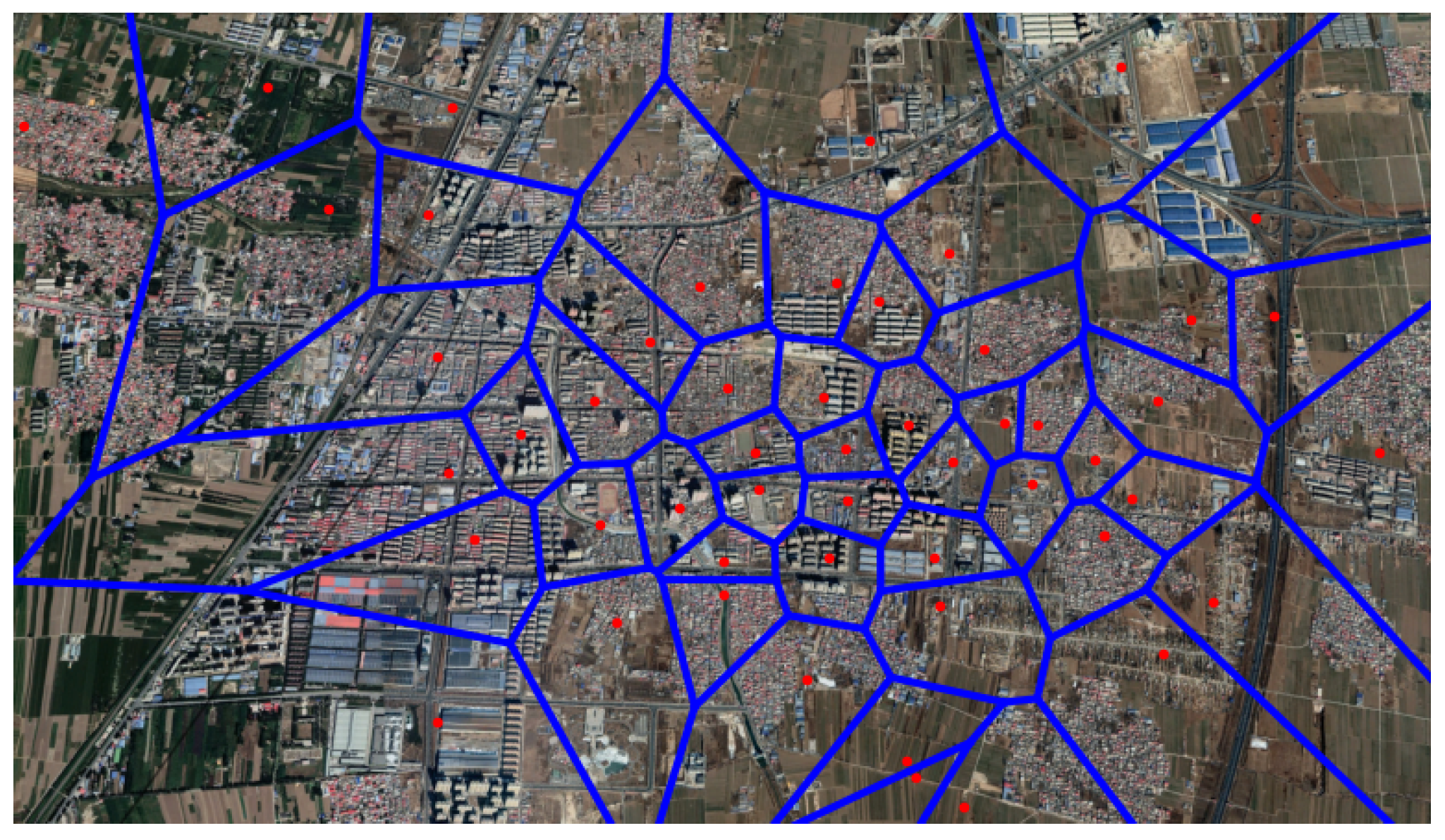
• We adopt Voronoi diagrams to zone urban areas by combining BS locations data and remote sensing images. The Voronoi-diagram-based method can accurately identify activity areas of the users served by BSs.
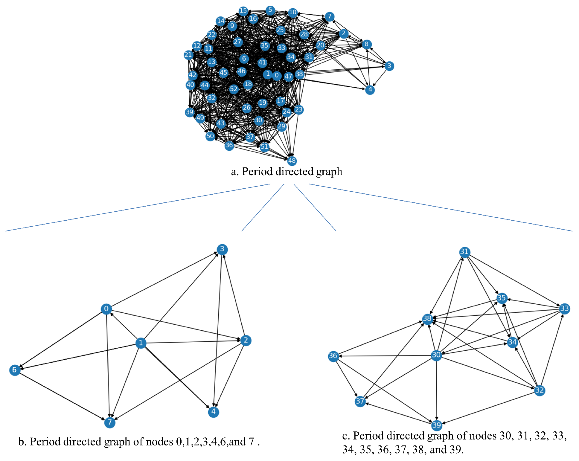
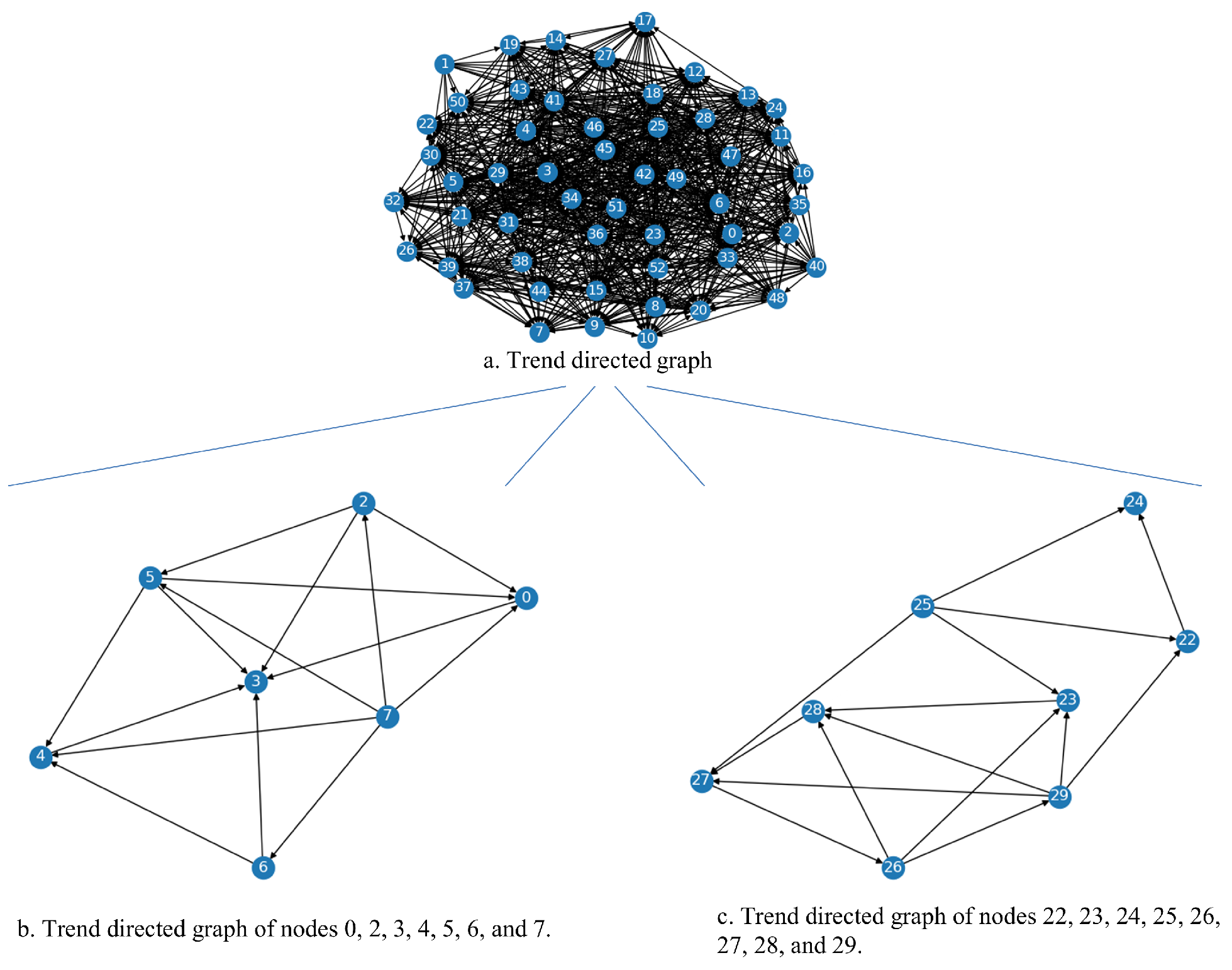
• We employ an ensemble empirical mode decomposition (EEMD) method to extract period component and trend component of wireless network data, which represent human behavior and activity level, and we use transfer-entropy-based causal structure learning to model urban function structure as a causal directed graph.
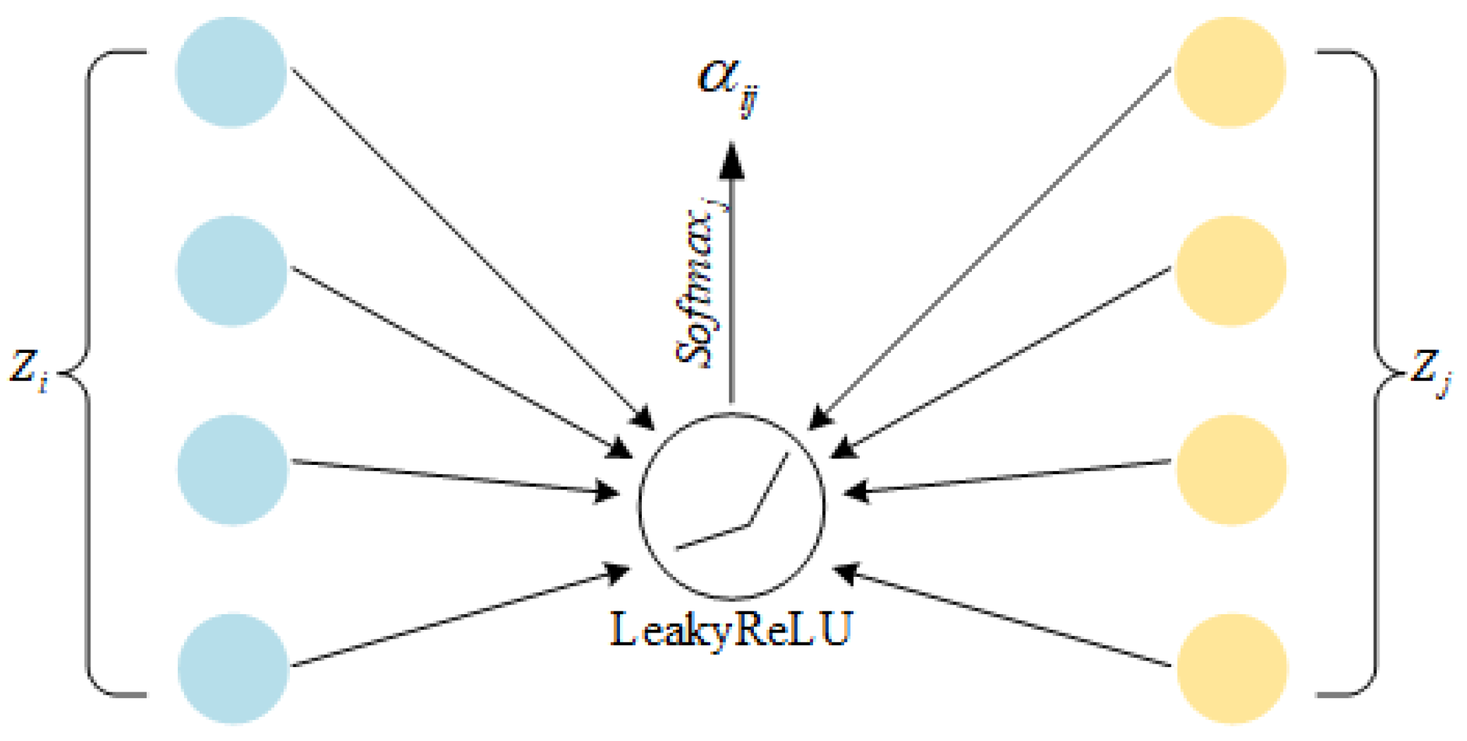
• We design a novel spatiotemporal city computing method based on graph attention network to mine features of urban function structure. The goal of our city computing research is to find an accurate prediction method for urban wireless traffic, which is an important topic in city simulation. Combined with commuting index calculation, the method can provide guidance for urban planning, transportation planning, and urban energy saving. Experimental results prove that the proposed method outperforms other common methods.

2. Materials and Methods

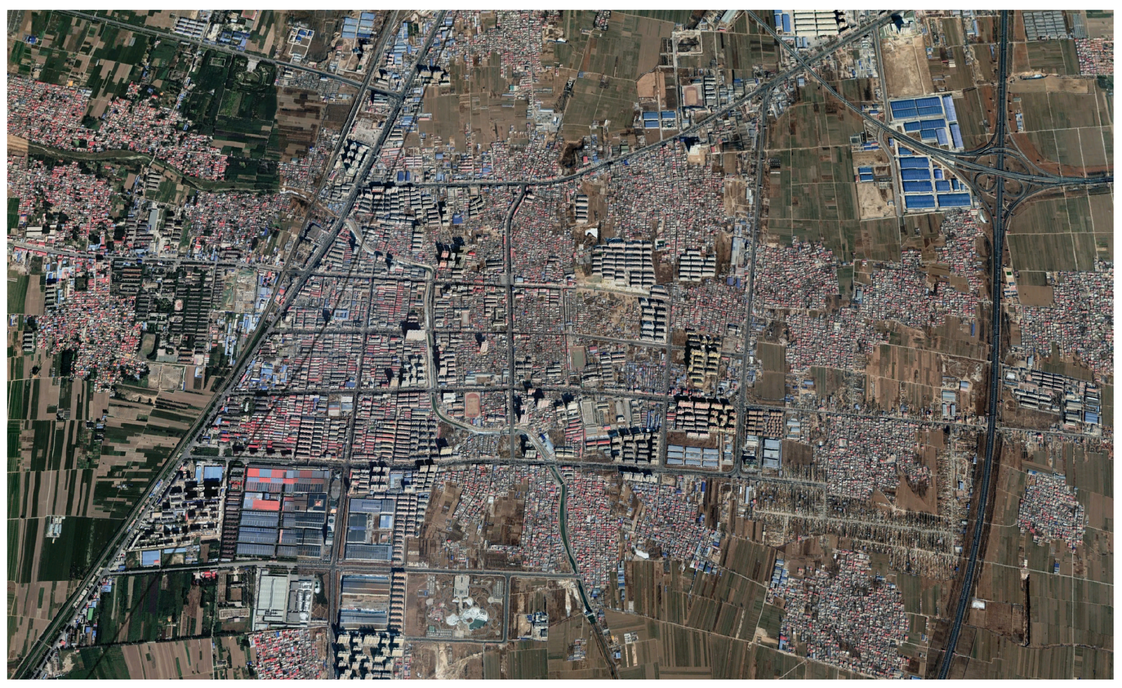
2.1. Dataset and Study Area

In this study, we selected Xushui District, Baoding City, Hebei Province, China, as the study area. Specifically, as shown in Figure 1, the study area ranges from longitude ${115.609}^{\circ }$E to ${115.695}^{\circ }$E and latitude ${38.994}^{\circ }$N to ${39.044}^{\circ }$N, covering approximately 39.057 km${}^2$. The study area belongs to Baoding city, which has a complex function. Moreover, there is no clear division of function zones in area, and a zone often contains many urban facilities, such as government agencies, investment enterprises, factories, schools, supermarkets, etc. It is a challenge to analyze urban function features in such a complex area.

The base-station-level wireless network data used in this paper were provided by a local mobile network operator. In total, we collected 62 days of downlink traffic data from 52 BSs in the study area. The temporal granularity of the data is 1 h, which means that one BS can generate 24 downlink traffic records data in a day. To make the presentation more concise, we show the data fields and partial contents in

Table 1. Structure of wireless network data.

Time Stamp	eNodeBID	Downlink Traffic (GB)
1 July 2019 00:00	1	2.429
1 July 2019 01:00	1	0.9914
1 July 2019 02:00	2	2.045
1 July 2019 03:00	2	0.2787
...

. The fields TimeStamp, eNodeBID, and Downlink Traffic represent the data collection time, the BS ID, and the sum of downlink traffic at a BS within 1 hour, respectively. For example, the second line of Table 1 means that the sum of downlink traffic volume at BS 1 is 0.9914 GB during 1 July 2019 00:00 and 1 July 2019 01:00.

To demonstrate spatial and temporal variation of the data, we plotted the temporal domain and spatial distribution of downlink traffic for partial BSs, as shown in Figure 2 and Figure 3. From Figure 2, we can see that the traffic variation trends of different BSs are generally similar within a day, but differ significantly at some time points. For example, from 14:00 to 16:00, the traffic trends of the two BSs are opposite. Figure 3 shows the variation of the traffic spatial distribution at different time points, where the square represents a BS, and the color of a square represents the volume of base-station-level (BS-level) downlink traffic. It can be seen that the spatial distribution of traffic also varies with time.

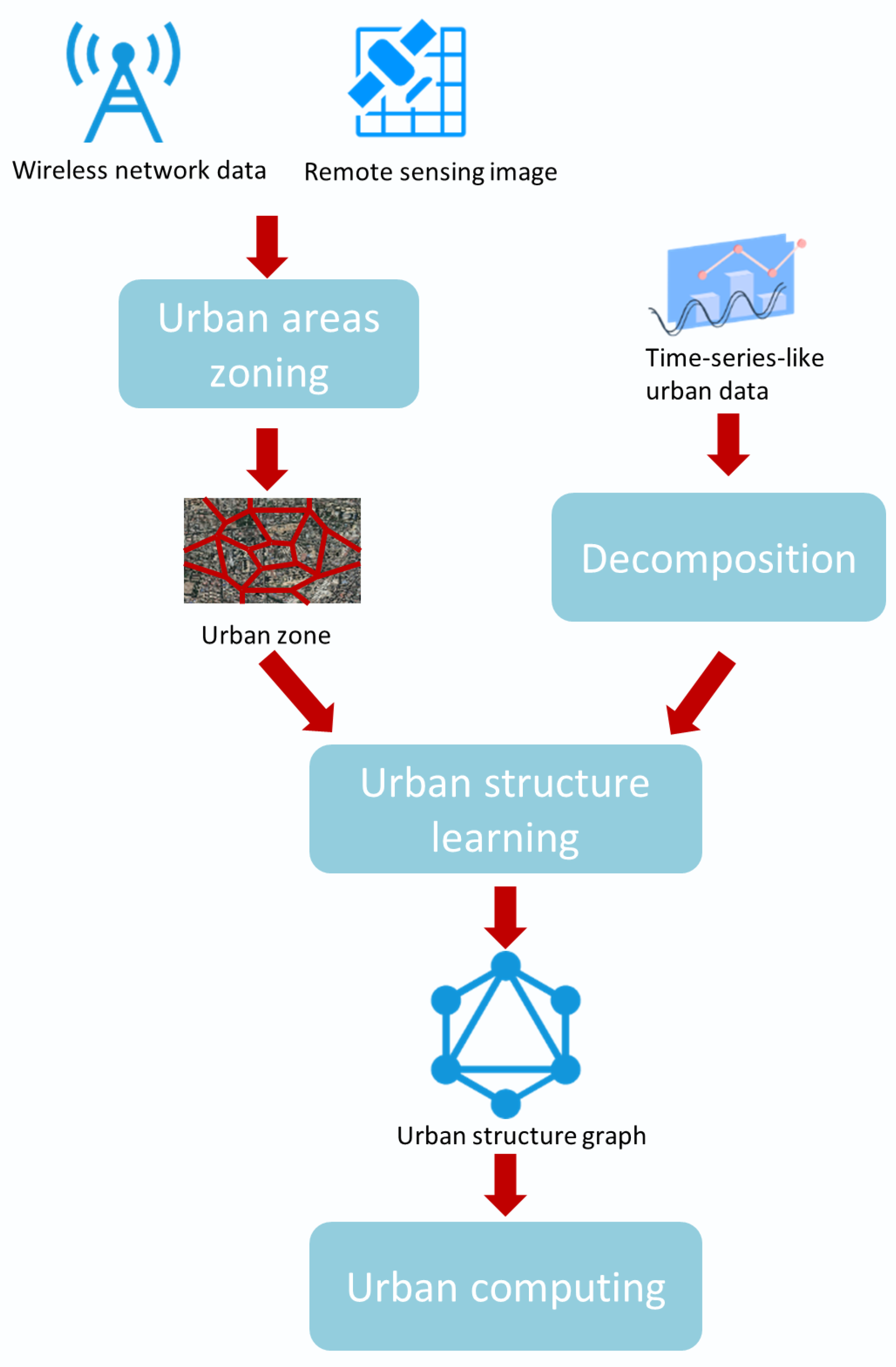
2.2. General Structure of Proposed Method

In order to make the presentation more concise, we describe the overall process of the proposed method before presenting the details. As shown in Figure 4, this article first analyzes city function structure and proposes a spatiotemporal city computing method based on city function structure. Modules of the process include urban area zoning, wireless network data decomposition, urban structure learning, and urban computing. Their functions are described as follows.

• Urban areas zoning: The motivation of this paper is to analyze city functions through BS-level wireless network traffic data. Therefore, the first task is to accurately zone BS coverage areas. As a result, an urban remote sensing image is divided into a collection of coverage areas anchored by BSs. To achieve this objective, we propose a Voronoi-diagram-based method, which is detailed in Section 2.3.
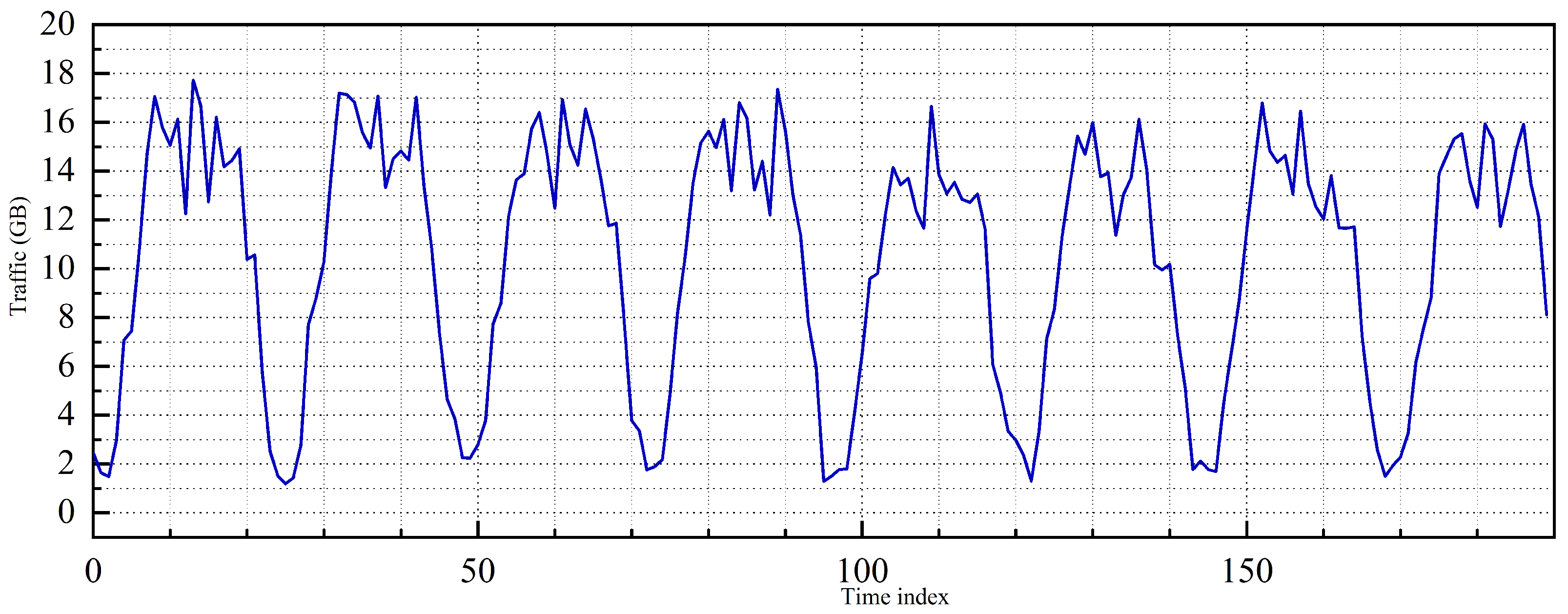
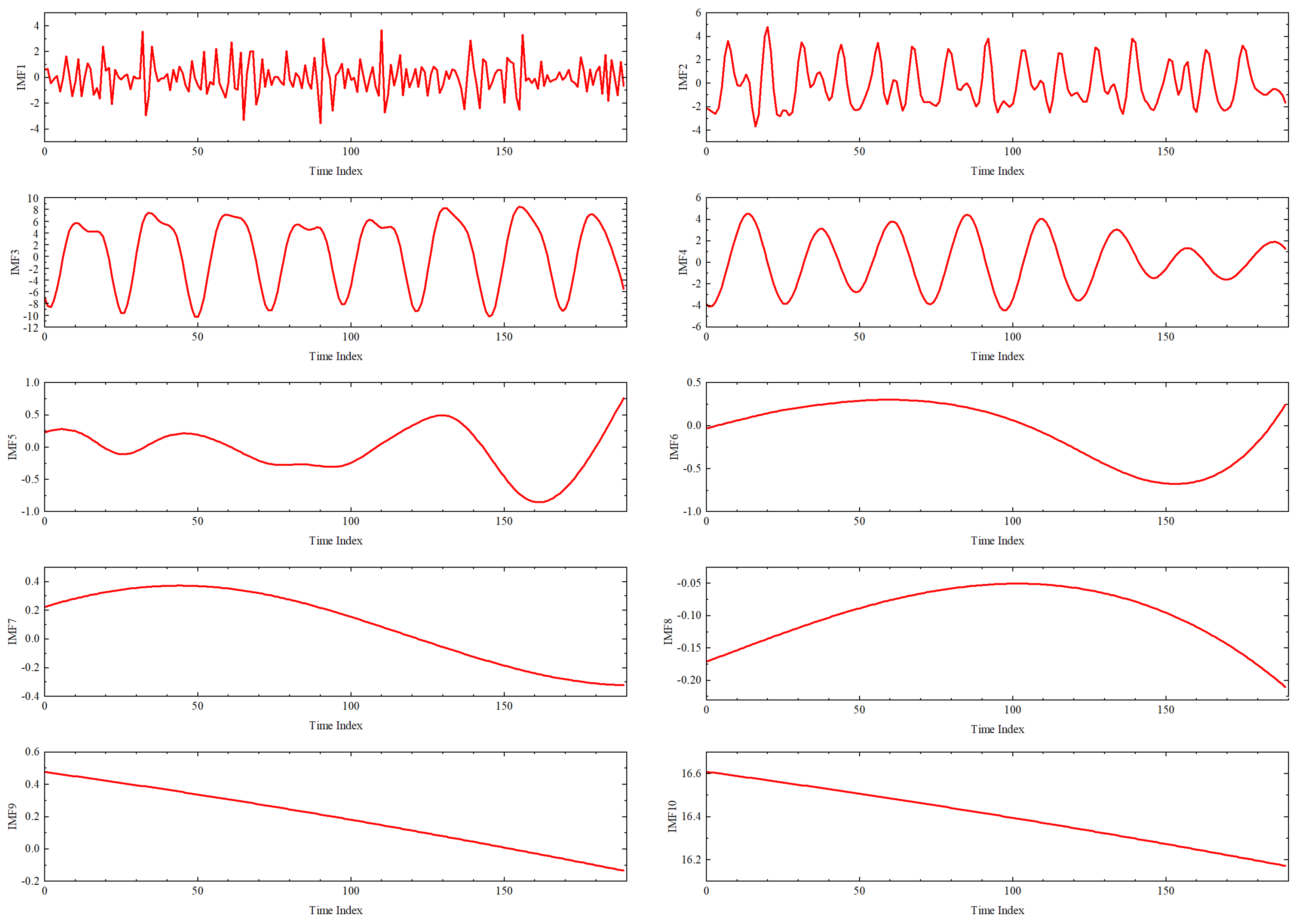
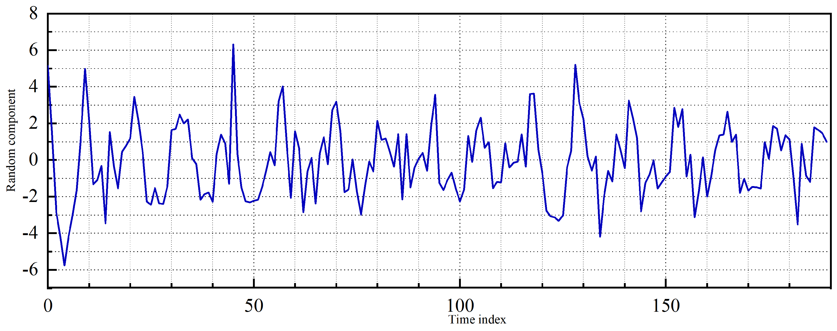
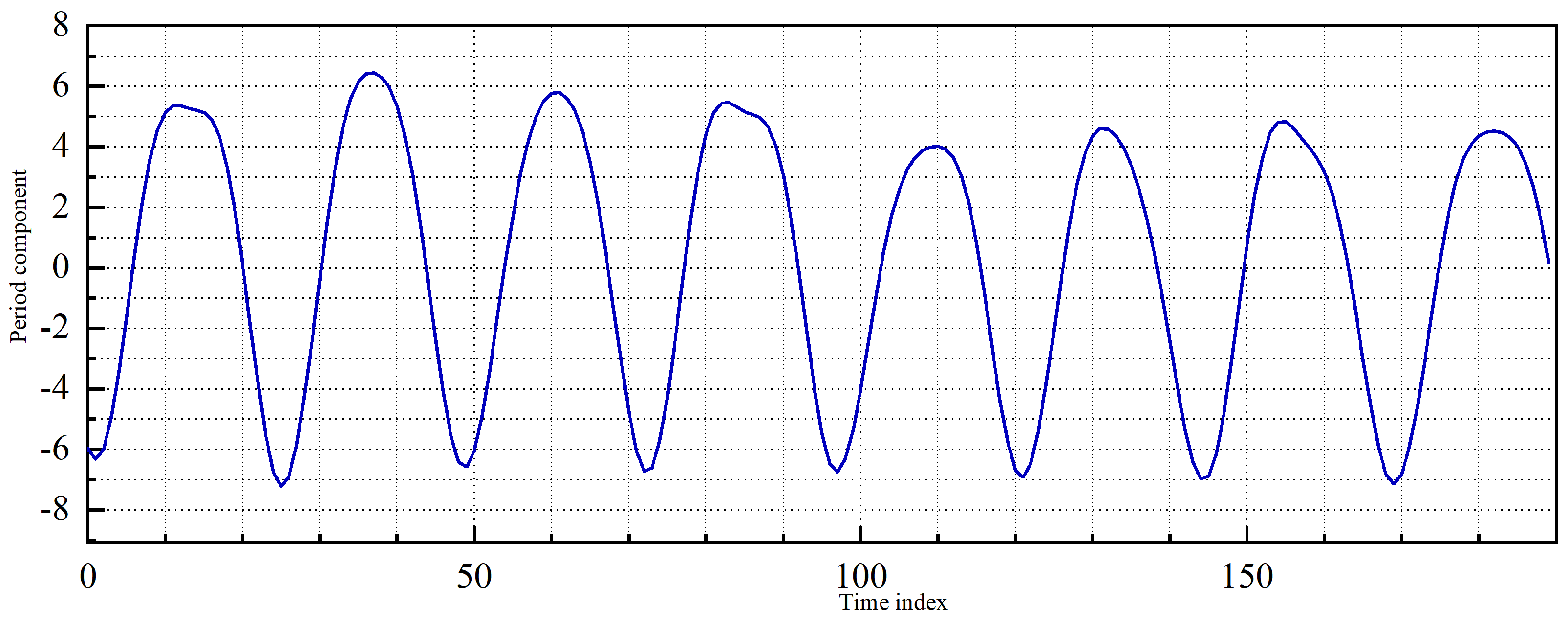
• Wireless network data decomposition: A challenge of analyzing urban function structure through wireless network data is the nonstationarity of the data. Therefore, as preparation for urban function structure learning, we propose an EEMD-based method for decomposing wireless network traffic data. The method decomposes nonstationary traffic time series of each BS into three components (i.e., random component, periodic component, and trend component). Each component represents human behavior at different scales within the BS coverage area. The specific process of the method is described in Section 2.4.1.
• Urban structure learning: In this module, we model the impacts among different coverage areas as directed causal relationships, and we adopt a VLTE-based causal structure learning method to mine the causal relationships among coverage areas at three components (the specific algorithm is described in Section 2.4.2). As a result, urban function structures at three component scales are modeled as causal directed graphs. This enables visualization of urban function structure.
• Urban computing: The above three modules provide the possibility for structured city simulation. To deal with complex causal directed graphs of urban areas, this paper introduces advanced graph neural network technology to implement spatiotemporal city computing, and we perform wireless network traffic prediction to verify the method. The spatiotemporal city computing method and simulation results are presented in Section 2.5 and Section 3.

2.3. Urban Area Zoning

In recent years, with the advancement of telecommunication technology, wireless data traffic services have become an essential part of people’s work and life. Therefore, in this paper, we analyze human activities in urban areas by using wireless traffic data. For user privacy protection, the data we selected are at BS-level. Thus, it is necessary to combine BS location, BS coverage, and remote sensing images to zone an urban area. Moreover, the zoning requires that all users in the zone are served by a single BS in the same zone. In order to achieve this requirement, we designed a zoning method for urban area based on a Voronoi diagram.

The service BS of wireless network users is generally the BS with the highest signal strength. The strength of a wireless signal is proportional to the distance from the user to the BS. Consider the BS as the control point of a Voroni diagram. The Voronoi diagram has a characteristic that the distance from any point within a Voronoi diagram to the control point of the diagram is smaller than the distance to control points of other diagrams. Therefore, the Voronoi diagram is a commonly used method to evaluate coverage of wireless networks. Considering the BS set $B=\{b_1,b_2,\dots ,b_N\}$ as control points, the Voronoi diagram of $b_i$ can be expressed as:

$$v\left(b_i\right)=\left\{x\mid ∥x-b_i∥\le ∥x-b_j∥\mathrm{for}j\ne i,j\in \{1,2,\dots ,N\}\}\right.$$

(1)

where $∥·∥$ means distance calculation, x means the point in the remote sensing image, and the set of Voronoi diagrams is described by $V=\{v\left(b_1\right),v\left(b_2\right),\dots ,v\left(b_N\right)\}$.

According to articles [43,44], we use the Delaunay triangulation [45] based method to generate Voronoi diagrams. The specific steps are as follows.

• Construct the Delaunay triangle network $T=\{t_1,t_2,\cdots \}$ according to control points set B and record the three control points that construct the triangle in T;
• Generate an adjacent triangle set $a\left(b_i\right)$ for each control point $b_i$, that is, $a\left(b_i\right)$ is the set of triangles whose vertices have control point $b_i$; then sort the triangles in $a\left(b_i\right)$ into a clockwise or counterclockwise direction;
• Calculate the external circle center of each triangle in T. Record it as $c\left(t\right),t\in T$;
• According to adjacent triangles of each control point, the Voronoi diagram set V are obtained by connecting outer circle centers of these adjacent triangles. The vertices of $v\left(b_i\right)$ can be represented by Formula (2). For Voronoi diagrams at the edges of the triangular network, a vertical bisector can be made to intersect with the outline of the figure and form a Voronoi diagram together with the outline.

$$vertices\left[v\left(b_i\right)\right]=\{c\left(t\right)\mid t\in a\left(b_i\right)\}$$

(2)

The Voronoi diagram offers the possibility of using BS-level data for urban function analysis. Compared with popular grid-level data, BS-level data can provide better protection of user privacy, because the construction of grid-level data often requires collecting user location information, and BS-level data aggregate all user data within coverage area, which avoids involving sensitive location information of users. On the other hand, many users often do not give third-party location permission or do not upload location information to protect privacy. Thus, grid-level data may miss the relevant information on human activities.

After zoning the remote sensing image by the Voronoi-diagram-based method, we can analyze urban area function features by the wireless network downlink traffic data of control points (i.e., BSs) within zones. In this study, we introduce zone commuting index $I_{v\left(b_i\right)}$ to analyze urban function features [46], which indicates the bias of zone $v\left(b_i\right)$ in terms of work and residence attributes, as shown in Equation (3).

$$I_{v\left(b_i\right)}=\left\{\begin{array}{cc}\frac{D_{\mathrm{mi}}\left(b_i\right)-D_{\mathrm{ci}}\left(b_i\right)}{{max}_{b_j\in B}\left(D_{\mathrm{mi}}\left(b_j\right)-D_{\mathrm{ci}}\left(b_j\right)\right)},\hfill & D_{\mathrm{mi}}\left(b_i\right)-D_{\mathrm{ci}}\left(b_i\right)>0\hfill \\ \frac{D_{\mathrm{mi}}\left(b_i\right)-D_{\mathrm{ei}}\left(b_i\right)}{{min}_{b_j\in B}\left(D_{\mathrm{ei}}\left(b_i\right)-D_{\mathrm{mi}}\left(b_i\right)\right)},\hfill & D_{\mathrm{mi}}\left(b_j\right)-D_{\mathrm{cj}}\left(b_i\right)<0\hfill \end{array}\right.$$

(3)

where $D_{mi}\left(b_i\right)$ denotes average hourly traffic increment of zone $v\left(b_i\right)$ in morning peak (i.e., 7:00 to 9:00), and $D_{ei}\left(b_i\right)$ denotes average hourly traffic increment of zone $v\left(b_i\right)$ in evening peak (i.e., 18:00 to 20:00). From Equation (3), it can be seen that $I_{v\left(b_i\right)}$ takes values in the range $[-1,1]$. As $I_{v\left(b_i\right)}$ is close to $-1$, zone $v\left(b_i\right)$ prefers to be considered as a residence. As $I_{v\left(b_i\right)}$ is close to 1, zone $v\left(b_i\right)$ prefers to be considered as a working place.

2.4. Urban Function Structure Learning

In the previous section, we used a Voronoi-diagram-based method for urban area zoning and introduced commuting index to analyze zone function feature. In this section, in order to further analyze function features of urban areas, we perform urban function structure learning based on the area zoning results in the previous section. Urban function structure learning aims at mining the relationship among urban remote sensing image zones by analyzing human-activity-related data. In this paper, human-activity-related data are BS-level wireless network downlink data, and we design an urban function structure learning method based on signal decomposition. First, the method decomposes wireless network data into three components, which represent different features of human activity. Second, a causal structure learning method is used to mine the relationship among different zones, and then model urban function structure as a causal directed graph.

2.4.1. Wireless Network Data Decomposition

Wireless network traffic data often show the characteristics of complex and nonstationary [47]. It is difficult to mine human activity information from the raw data. Therefore, in this paper, we introduced EEMD [48,49] to decompose traffic data into three components, which are random component, period component, and trend component. The random component represents the random actions of humans. The period component represents regular periodic productive activities of humans in urban life. The trend component represents the level of human activity in the zone.

EEMD is an improved method of empirical mode decomposition (EMD). EMD was originally proposed by N.E. Huang to adaptive analyze nonlinear and nonstationary signals [50]. Compared with EMD, EEMD eliminates the problem of mode mixing by adding white noise to the original signal. This technique is feasible for wireless network traffic data decomposition [51]. To comprehensively describe EEMD, we first introduce the concept of intrinsic mode functions (IMF). IMF is a series that satisfies two conditions:

• The number of extreme and zero crossings must either equal or differ by 1 or 2;
• The envelopes defined by the local maxima and the local minima are symmetrical.

The EEMD algorithm assumes that time series data generally contain multiple volatility components which can be expressed by the IMF function, and the motivation for adding white noise is to make the signals of different scales reside in the corresponding IMFs.

We denote the traffic data of BS i by $S_i$ and the total wireless network traffic data by $S=\left[S_1,S_2,\dots S_i\dots S_N\right]$, where N is the number of BSs. The process of EEMD based decomposition for each $S_i$ is described as follows:

• Initialize $l=1$ and $r_0\left(t\right)=S_i$.
• Generate M white noises $n_j\left(t\right),m=1,2,\dots ,M$.
• Perform the jth decomposition on the signal added white noise.

  a

  As shown in Formula (4), add a white noise to $r_{l-1}\left(t\right)$.

  $$x_j\left(t\right)=r_{l-1}\left(t\right)+n_j\left(t\right)$$

  (4)

  b

  Set $k=1$, and initialize $h_{j,k-1}=x_j\left(t\right)$.

  c

  Extract the upper envelope $M_u$ and lower envelope $M_l$ of $h_{j,k-1}$, and $h_{j,k}$ can be obtained by (5),

  $$h_{j,k}\left(t\right)=h_{j,k-1}-m_j\left(t\right)$$

  (5)

  where $m_j\left(t\right)=(M_u+M_l)/2$.

  d

  If $h_{j,k}$ is an IMF, then set $IM{F}_j=h_{j,k}$, otherwise go to step (c) with $k=k+1$.

• Set $j=j+1$ then repeat step 2 if $j<=M$.
• Calculate the mean of IMFs by Formula (6).

  $$\overline{IM{F}_l}=\frac{1}{M}\sum _{j=1}^{M}IM{F}_j$$

  (6)

  Due to the zero mean property of white noise, Formula (6) removes the effect of the added noise volume on the original signal.
• Report $\overline{IM{F}_l}$ then separate $\overline{IM{F}_l}$ from $r_{l-1}$ to obtain $r_l\left(t\right)$.

  $$r_l\left(t\right)=r_{l-1}\left(t\right)-IM{F}_l$$

  (7)
• If $r_l\left(t\right)$ still has least 2 extremes then set $l=l+1$ and repeat the operations from step 2 to step 6, otherwise the decomposition process is finished.

After decomposition, we cluster the IMF set $\{\overline{IM{F}_1},\overline{IM{F}_2},\dots \}$ of each $S_i$ into three components by K-nearest neighbor (KNN) algorithm, where sample entropy [52] and mean period [53] are used to represent the features of each IMF.

The frequency of IMF decreases with the increase of decomposition times j [53]. According to N.E. Huang’s research, the low-order and high-frequency IMFs can be regarded as noise. In cellular traffic data, noise represents the random component due to user service requests. The trend component which consists of high-order IMFs represents the growth or decline trend of traffic. The frequency of period component is between random and period component, which stands for the tidal characteristic of cellular traffic.

2.4.2. Causal Structure Learning

In this section, we analyze urban area function structure by learning the structure of period component and trend component. Causality is utilized to model the relationship among different zones. The causality describes how one time series impacts another time series, and many researchers have demonstrated its effectiveness [39,54]. In this study, the function feature of each zone is represented by time series (i.e., wireless network data), so the relationship among time series mined by causal structure learning describes the influence of human activities among different zones.

At present, the common causality test algorithms mainly include Granger causality and transfer entropy. The Granger causality test is a statistical hypothesis test which is used to determine whether one time series is valuable for predicting another [55], but the linear regression model in Granger causality test may not be able to capture the nonlinear process dynamics and may miss the causal connection [56]. The transfer entropy (TE) is a nonlinear extension of Granger causality [57]. They assume that a time series is influenced by a combination of other series with a fixed time delay. This assumption is too strong for many applications.

To mine causal relation deeply, we introduced the variable-lag transfer entropy (VLTE) method to learn the causal structure. Compared with the TE-based method, VLTE adaptively aligns two time series and mines the causal relationship between them [58,59]. This overcomes the problem of fixed time delay assumption. The calculation method of VLTE from time series X to Y is described by Formula (8):

$${\mathcal{T}}_{X\to Y}^{\mathrm{VL}}=H\left(Y\left(t\right)\mid Y_{t-1}^{\left(k\right)}\right)-H\left(Y\left(t\right)\mid Y_{t-1}^{\left(k\right)},{\tilde{X}}_{t-1}^{\left(l\right)}\right)$$

(8)

where $H(·\mid ·)$ is a conditional entropy, $Y_{t-1}^{\left(k\right)}=\{Y(t-1),\dots ,Y(t-k)\}$, and ${\tilde{X}}_{t-1}^{\left(l\right)}=\{X(t-1-{\Delta }_{t-1}),\dots ,X(t-l-{\Delta }_{t-l})\}$. The entropy used in this paper is Shannon entropy.

$$H\left(X\right)=-\sum _{t}p\left(X\left(t\right)\right){log}_2\left(p\left(X\left(t\right)\right)\right)$$

(9)

Now, our task is to find an appropriate series $\{{\Delta }_{t-1},{\Delta }_{t-2},\dots \}$ to reconstitute $X_{t-1}^{\left(l\right)}=\{X(t-1),\dots ,X(t-l)\}$ into ${\tilde{X}}_{t-1}^{\left(l\right)}=\{X(t-1-{\Delta }_{t-1}),\dots ,X(t-l-{\Delta }_{t-l})\}$. According to [59], dynamic time wrapping (DTW) is used for accomplishing this task. Then, we can obtain the causal relationship from X to Y by Formula (10):

$$C{S}_{X,Y}=\left\{\begin{array}{cc}\mathrm{true}\hfill & {\mathcal{T}}_{X\to Y}^{\mathrm{VL}}/{\mathcal{T}}_{Y\to X}^{\mathrm{VL}}>1\hfill \\ \mathrm{false}\hfill & {\mathcal{T}}_{X\to Y}^{\mathrm{VL}}/{\mathcal{T}}_{Y\to X}^{\mathrm{VL}}<1\hfill \end{array}\right.$$

(10)

The random component, period component, and trend component are denoted by $X^r=\{x_i^r\mid i\in \{1,2,\dots ,N\}\}$, $X^p=\{x_i^p\mid i\in \{1,2,\dots ,N\}\}$, and $X^t=\{x_i^t\mid i\in \{1,2,\dots ,N\}\}$. $x_i^{*}(\ast =r,p,ort)$ is the corresponding component time series of zone $v\left(b_i\right)$, which is obtained in Section 2.4.1. In this study, we analyze the function structure of urban area at three levels: random structure $D_r=(X^r,E^r)$, periodic structure $D_p=(X^p,E^p)$, and trend structure $D_t=(X^t,E^t)$. $D_{*}=(X^{*},E^{*})(\ast =r,p,ort)$ is a directed graph where the vertices are the corresponding component of zones, and the directed edges represent the influence among zones. The specific generation steps of edge $E^{*}$ are shown in Algorithm 1. These three structures not only describe the influence among zones but also assist in city computing to improve the performance of the method, which is described in the next section.

Algorithm 1 Causal structure learning.

1: Input $X^{*}=\{x_i^{*}\mid i\in \{1,2,\dots ,N\}\}(\ast =r,p,ort)$ 2: Initialize $E^{*}={\left[e_{i,j}^{*}\right]}_{N\times N}$ to identity matrix 3: for $i=1,2,\dots ,N$ do 4:     for $j=1,2,\dots ,N$ and $j\ne i$ do 5:         $X\leftarrow x_i^{*}$ 6:         $Y\leftarrow x_j^{*}$ 7:         Calculate ${\mathcal{T}}_{X\to Y}^{\mathrm{VL}}$ by Equation (8) 8:         Calculate ${\mathcal{T}}_{Y\to X}^{\mathrm{VL}}$ by Equation (8) 9:         Calculate $C{S}_{X,Y}$ by Equation (10) 10:         $e_{i,j}^{*}\leftarrow C{S}_{X,Y}$ 11:     end for 12: end for 13: Output $E^{*}$

Finally, we obtain the directed causal graph of each component, which can be expressed as follows: $D_T=(X^t,E^t)$, $D_P=(X^p,E^p)$, and $D_R=(X^r,E^r)$. Taking the trend component as an example, $X^t=\{x_i^t\mid i\in BSset\}$ is the node set, $x_i^t$ is the trend component obtained by Section 2.1, and $E^t$ is the set of edges indicated by adjacency matrix $A^t={\left[C{S}_{x_i^t,x_j^t}\right]}_{N\ast N}$, where N is the number of BSs.

2.5. Spatiotemporal City Computing

For urban simulation, this section proposes a spatiotemporal city computing process based on the previous analysis of urban area function, as shown in Figure 4. The method extracts spatial and temporal features of time-series-like urban data and performs prediction. The prediction results can help urban planners perceive changes in urban development and realize advanced planning. The data preprocessing part of this method is the same as the data decomposition and structure learning introduced in Section 2.3 and Section 2.4. The data decomposition can be considered as temporal feature extraction, and the structure learning can be considered as spatial feature extraction. A deep learning method based on GAT is introduced in the urban computing part for deeper spatiotemporal features mining and predicting. To make the presentation more concise, the following will introduce the deep learning method from the perspective of wireless network traffic prediction.

Recently, the rise of graph neural networks has successfully promoted the research of data mining. It makes up for the shortcomings of neural networks in dealing with non-Euclidean spatial data (graph data), so GAT [60] is used to extract features from the graph data generated in the previous section. The attention mechanism in GAT learns different weights for different neighbor nodes, which greatly improves the expression ability of graph neural network models by aggregating the causality between nodes into the prediction model.

Specifically, the input of GAT is $h=\left\{h_1,\dots ,h_i,h_N\right\}$, where $h_i$ represents the component series of BS i.

Specifically, the input of GAT is $D_{*}=(X^{*},E^{*}={\left[e_{i,j}^{*}\right]}_{N\times N})(\ast =r,p,ort)$. $z_i$ represents the embedding of nodes i (i.e., zone $v\left(b_i\right)$), which is calculated by Formula (11).

$$z_i=W{x}_i^{*}$$

(11)

where W is a parameter that needs to be learned. The attention mechanism is described in Figure 5. ${\alpha }_{ij}$ is the normalized attention coefficient which represents the effect of neighbor node j to target node i. The calculation process of ${\alpha }_{ij}$ can be written as Formulas (12) and (13).

$$p_{ij}=LeakyReLU\left({\overrightarrow{a}}^T\left(z_i\parallel z_j\right)\right)$$

(12)

$${\alpha }_{ij}=softmax\left(p_{ij}\right)=\frac{exp\left(p_{ij}\right)}{{\sum }_{e_{j,i}^{*}\ne 0}exp\left(p_{ik}\right)}$$

(13)

where ${\overrightarrow{a}}^T$ is a feedforward neural network whose parameters need to be learned. $LeakyReLU(·)$ is nonlinear activation function, $softmax(·)$ is normalization function, and ‖ means concatenated. GAT extracts the feature of each node depending on the nodes which have a causal correlation with the target node. Therefore, directed causal structure is embedded into the neural network and used for prediction, and corresponding formulas are (14).

$${\overrightarrow{h}}_i=\sigma \left(\sum _{e_{j,i}^{*}\ne 0}{\alpha }_{ij}{z}_j\right)$$

(14)

After graph feature extraction, we input the features ${\overrightarrow{h}}_i$ into the GRU to obtain component prediction result $\overline{X^{*}}$. As a variant of LSTM, GRU has a similar concept [61], which uses the reset gate and the update gate to capture the temporal dependence. Finally, we obtain the prediction result of wireless network traffic by summing up the prediction of each component, as shown in Equation (15).

$$\overline{S}=\overline{X^t}+\overline{X^p}+\overline{X^r}$$

(15)

3. Results

3.1. Urban Area Zoning

As introduced in Section 2.2, we propose an urban area zoning method based on remote sensing image and wireless network data. The remote sensing image of the study area is shown in Figure 1. Wireless network BS locations are provided by local operators. The zoning result is shown in Figure 6, where the red dots are the BS locations and the blue lines are zone segmentation lines. Further, we calculate the commuting index for each zone by using Equation (3). The results are shown in

Table 2. Commuting index.

Zone Id	Commuting Index	Zone Id	Commuting Index	Zone Id	Commuting Index
1	0.14713343	18	0.6250174	35	−0.905465
2	0.003361332	19	−0.055667	36	−0.970327
3	−0.504959471	20	−0.550208	37	−0.576254
4	−0.487725772	21	−0.949675	38	−0.860672
5	−0.894548963	22	−0.165399	39	−0.561098
6	0.250310568	23	−0.79184	40	−0.558165
7	0.462387708	24	0.1178097	41	−0.658584
8	−0.490481698	25	−0.434763	42	−0.626709
9	−0.819941458	26	−0.922275	43	−0.805434
10	1	27	−0.661987	44	−0.33808
11	0.062685314	28	−0.727245	45	−0.621166
12	−0.335140768	29	−0.940734	46	0.0613054
13	−0.155702131	30	−0.610347	47	−0.689869
14	−0.368456079	31	−0.191953	48	−0.868152
15	−0.155143688	32	−0.902722	49	0.7691417
16	−0.66856836	33	−0.444718	50	−0.316654
17	−0.669408032	34	−0.55769	51	−0.028517
				52	−0.541641

.

3.2. Urban Function Structure

As introduced in Section 2.3, we propose an urban function structure learning method based on time series decomposition and causal structure learning. A certain zone is taken as an example. EEMD-based time series decomposition decomposes the base-station-level downlink traffic data in a zone (shown in Figure 7) into 10 IMF time series, as shown in Figure 8.

After that, we use the KNN algorithm to cluster IMF series into three components based on their sample entropy and average period. The random component, the period component, and the trend component are represented in Figure 9, Figure 10 and Figure 11, respectively.

Finally, we use causal structure learning to model urban function structure as period and trend structures, as shown in Figure 12 and Figure 13. Due to the complexity of the study area, the structure of the directed graph is complex. For better presentation, we amplify the graph of some neighboring zones, as shown in Figure 12b,c and Figure 13b,c. The nodes in Figure 12 and Figure 13 represent zone IDs, and the directed edges represent influence among zones. For example, in Figure 12b, the directed edge between zones 0 and 5 represents the impact of zone 0 on zone 5.

3.3. Spatiotemporal City Computing

In this section, we verify the effectiveness and efficiency of the proposed city computing process from the perspective of wireless network traffic prediction. We compare the experimental results with other common methods. The granularity of traffic data is 1 hour, and a total of 62 days are counted (July 2019 to August 2019). Actual traffic data were collected at 52 BSs in the study area. We use the data of 4 hours to predict the traffic for the next hour. In model training, the ratio of the training set is 0.87, and the training parameters are shown in

Table 3. Training parameters.

Component	Learning Rate	Batch Size	Iterations
Trend	0.08	128	800
Period	0.007	64	800
Random	0.01	128	800

. Since three components have different patterns and jitter levels, the training parameters for them are also different. The parameters in Table 3 are the optimal parameters obtained through extensive experiments. In order to clearly describe the performance of different algorithms, RMSE and MAPE are calculated. To verify the performance of the proposed method, we compare it with three advanced methods.

• GCN: GCN is a convolutional neural network for graph data [10]. In the simulation of this method, the used graph structure is generated by the urban function structure learning module proposed in this paper.
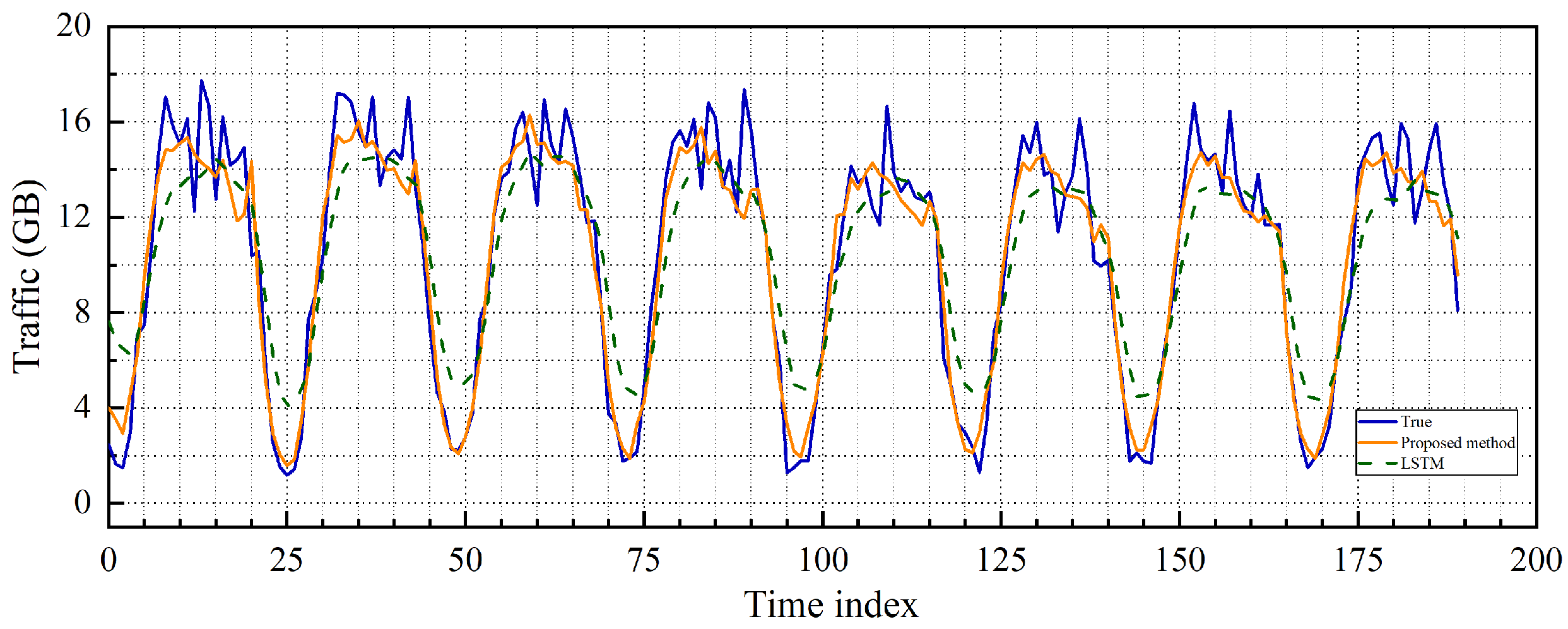
• LSTM: LSTM is a recurrent neural network with long- and short-term memory capability. In recent years, it is often used to perform time series prediction with the spread of machine learning applications [62].
• ARIMA: ARIMA is a differentially integrated moving average autoregressive model, which is a statistical method commonly used for time series prediction.

The comparison result is presented in

Table 4. Performance comparison.

Method	RMSE	MAPE
Proposed method	1.535814	45.895
GCN	1.603046	55.4792
LSTM	2.0889	55.5947
ARIMA	3.020975	87.8763

. It is obvious that the performance of our proposed DIVC-GAT is the best. To better show the performance of the proposed method, the prediction result of a certain BS is used as an example, as shown in Figure 14.

4. Discussion

As can be seen from Figure 6, the zone density is high in the urban center and low around the town. This is because operators deploy a large number of BSs in urban centers to guarantee the user experience of a dense population. From the perspective of city function analysis, the dense population and complex functions of city centers require fine-grained area zoning. Fine-grained zoning can improve the accuracy of urban function analysis. Conversely, in the sparsely populated areas around urban areas, we can expand the size of zones. It can be seen that the introduction of wireless network data can help in function analysis of urban areas. Table 2 shows zone commuting indices calculated from wireless network data. It can be seen that 10 zones have a commuting index greater than 0, 29 zones have a commuting index less than −0.5, and 14 zones have a commuting index greater than −0.5 and less than 0. This indicates that the urban area consists of a few commercial centers, some mixed zones, and mostly residential areas.

The time series in Figure 8 are arranged from top to bottom by the order of decomposition. It can be seen that IMF series are more smooth with higher order. This is because the EEMD algorithm can be regarded as a filter, and as order increases, the filtered series is more stable. Further, IMF series can be clustered into three components by the KNN algorithm, as shown in Figure 9, Figure 10 and Figure 11. The IMF series with lower order are summed to obtain a jittered random component. The higher-order ones are summed to obtain a trend component. The rest of them are summed to form a period component. The period component and trend component represent human behavior and activity, respectively, so their structures are not the same, as shown in Figure 12 and Figure 13, and by enlarging the structure graph of the neighboring area, urban planners can gain insight into the changes of people’s behavior and activity across zones. Taking Figure 13b as an example, we can see that the development of area is proceeding to zone 3 and zone 0. This is because all edges of both zones point to themselves.

From Figure 12 and Figure 13, we can see that the function structure of the study area is very complex. For urban simulation, the city computing method proposed in Section 2.4 adopts GAT to handle complex graph structure data. We verify the urban simulation by performing wireless network traffic prediction. As shown in Table 4, the performance of GCN and the proposed method is significantly better than that of LSTM and ARIMA. This proves that the incorporation of urban structured information can effectively improve the performance of urban computing. Further, our proposed method is better than GNN. The attention mechanism in GAT embeds the direction of causality into city computing and enhances the depth of spatial relation mining among different coverage areas.

Compared with LSTM and ARIMA, which cannot handle structural information, the proposed method achieves joint processing of multiple zones through attention mechanism and improves the performance of city computing.

Moreover, as shown in Figure 14, the proposed method has a higher performance gain at inflection points where traffic changes drastically. This further demonstrates superiority of the spatiotemporal urban computing method.

With the above analysis, our proposed method achieves extraction of human activity features and visualization of urban function structure while ensuring user privacy. Combined with spatiotemporal urban computing, relevant authorities can make active sense of urban areas and predict the evolution of urban human activity. This provides structured information and human activity trend information for urban planning, which improves the effectiveness and science of planning decisions.

5. Conclusions

In this paper, we studied the application of remote sensing image and wireless network data to urban function analysis and proposed a spatiotemporal city computing method. Combining remote sensing images, we introduced the Voronoi diagram for urban area zoning, which is commonly used in network coverage analysis, and the function feature of each zone was evaluated by wireless network data. Further, we used causality to evaluate influence among zones and modeled urban function structure as causal directed graphs.

Urban simulation and prediction supported by remote sensing and wireless big data can realize the mining of urban dynamic changes. This paper proposes a novel spatiotemporal city computing method using remote sensing and wireless big data in urban research. The results show that this method can be used in urban planning, urban simulation, and other research fields. In addition, the resource consumption problem caused by the deployment of 5G can also be achieved through the analysis method of combining remote sensing information with wireless data to achieve environmentally friendly and sustainable urban development. In the future, our research will expand the scope of multisource data, such as city light data, road traffic data, and so on. Moreover, we will introduce gridded wireless network data for more detailed analysis of urban area function.

References

1. Zhou, W.; Pickett, S.T.; Cadenasso, M.L. Shifting concepts of urban spatial heterogeneity and their implications for sustainability. Landsc. Ecol. 2017, 32, 15–30. [Google Scholar] [CrossRef]
2. Shoemaker, D.A. The Role of Spatial Heterogeneity and Urban Pattern in Modulating Ecosystem Services; North Carolina State University: Raleigh, NC, USA, 2016. [Google Scholar]
3. Pickett, S.T.; Cadenasso, M.L.; Childers, D.L.; McDonnell, M.J.; Zhou, W. Evolution and future of urban ecological science: Ecology in, of, and for the city. Ecosyst. Health Sustain. 2016, 2, e01229. [Google Scholar] [CrossRef]
4. Borgström, S.; Andersson, E.; Björklund, T. Retaining multi-functionality in a rapidly changing urban landscape: Insights from a participatory, resilience thinking process in Stockholm, Sweden. Ecol. Soc. 2021, 4, 4. [Google Scholar] [CrossRef]
5. Elbakidze, M.; Dawson, L.; Milberg, P.; Mikusiński, G.; Hedblom, M.; Kruhlov, I.; Yamelynets, T.; Schaffer, C.; Johansson, K.E.; Grodzynskyi, M. Multiple factors shape the interaction of people with urban greenspace: Sweden as a case study. Urban For. Urban Green. 2022, 74, 127672. [Google Scholar] [CrossRef]
6. Shane, D.G. Urban Design since 1945. In A Global Perspective; John Wiley and Sons Ltd.: New York, NY, USA, 2011. [Google Scholar]
7. Ortiz-Báez, P.; Cabrera-Barona, P.; Bogaert, J. Characterizing landscape patterns in urban-rural interfaces. J. Urban Manag. 2021, 10, 46–56. [Google Scholar] [CrossRef]
8. Vanderhaegen, S.; Canters, F. Mapping urban form and function at city block level using spatial metrics. Landsc. Urban Plan. 2017, 167, 399–409. [Google Scholar] [CrossRef]
9. Yan, X.; Ai, T.; Yang, M.; Yin, H. A graph convolutional neural network for classification of building patterns using spatial vector data. ISPRS J. Photogramm. Remote Sens. 2019, 150, 259–273. [Google Scholar] [CrossRef]
10. Zhang, K.; Chuai, G.; Zhang, J.; Chen, X.; Si, Z.; Maimaiti, S. DIC-ST: A Hybrid Prediction Framework Based on Causal Structure Learning for Cellular Traffic and Its Application in Urban Computing. Remote Sens. 2022, 14, 1439. [Google Scholar] [CrossRef]
11. Gu, J.R.; Chen, X.W.; Yang, H.L. Spatial clustering algorithm on urban function oriented zone. Sci. Surv. Mapp. 2011, 36, 5. [Google Scholar]
12. Cheng, J.; Turkstra, J.; Peng, M.; Du, N.; Ho, P. Urban land administration and planning in China: Opportunities and constraints of spatial data models. Land Use Policy 2006, 23, 604–616. [Google Scholar] [CrossRef]
13. Chen, Y.; Yang, J.; Yang, R.; Xiao, X.; Xia, J.C. Contribution of urban functional zones to the spatial distribution of urban thermal environment. Build. Environ. 2022, 216, 109000. [Google Scholar] [CrossRef]
14. Heiden, U.; Heldens, W.; Roessner, S.; Segl, K.; Esch, T.; Mueller, A. Urban structure type characterization using hyperspectral remote sensing and height information. Landsc. Urban Plan. 2012, 105, 361–375. [Google Scholar] [CrossRef]
15. Batty, M.; Longley, P.A. Fractal Cities: A Geometry of Form and Function; Academic Press: Cambridge, MA, USA, 1994. [Google Scholar]
16. Luck, M.; Wu, J. A gradient analysis of urban landscape pattern: A case study from the Phoenix metropolitan region, Arizona, USA. Landsc. Ecol. 2002, 17, 327–339. [Google Scholar] [CrossRef]
17. Zhou, W.; Ming, D.; Lv, X.; Zhou, K.; Bao, H.; Hong, Z. SO–CNN based urban functional zone fine division with VHR remote sensing image. Remote Sens. Environ. 2020, 236, 111458. [Google Scholar] [CrossRef]
18. Aubrecht, C.; León Torres, J.A. Evaluating multi-sensor nighttime earth observation data for identification of mixed vs. residential use in urban areas. Remote Sens. 2016, 8, 114. [Google Scholar] [CrossRef]
19. Ben-Dor, E.; Levin, N.; Saaroni, H. A spectral based recognition of the urban environment using the visible and near-infrared spectral region (0.4-1.1 μm). A case study over Tel-Aviv, Israel. Int. J. Remote Sens. 2001, 22, 2193–2218. [Google Scholar] [CrossRef]
20. Herold, M.; Gardner, M.E.; Roberts, D.A. Spectral resolution requirements for mapping urban areas. IEEE Trans. Geosci. Remote Sens. 2003, 41, 1907–1919. [Google Scholar] [CrossRef]
21. Du, S.; Du, S.; Liu, B.; Zhang, X. Context-enabled extraction of large-scale urban functional zones from very-high-resolution images: A multiscale segmentation approach. Remote Sens. 2019, 11, 1902. [Google Scholar] [CrossRef]
22. Tu, W.; Hu, Z.; Li, L.; Cao, J.; Jiang, J.; Li, Q.; Li, Q. Portraying urban functional zones by coupling remote sensing imagery and human sensing data. Remote Sens. 2018, 10, 141. [Google Scholar] [CrossRef]
23. Cao, R.; Tu, W.; Yang, C.; Li, Q.; Liu, J.; Zhu, J.; Zhang, Q.; Li, Q.; Qiu, G. Deep learning-based remote and social sensing data fusion for urban region function recognition. ISPRS J. Photogramm. Remote Sens. 2020, 163, 82–97. [Google Scholar] [CrossRef]
24. He, Y.; Wang, W.; Chen, Y.; Yan, H. Assessing spatio-temporal patterns and driving force of ecosystem service value in the main urban area of Guangzhou. Sci. Rep. 2021, 11, 3027. [Google Scholar] [CrossRef]
25. Song, J.; Lin, T.; Li, X.; Prishchepov, A.V. Mapping urban functional zones by integrating very high spatial resolution remote sensing imagery and points of interest: A case study of Xiamen, China. Remote Sens. 2018, 10, 1737. [Google Scholar] [CrossRef]
26. Huang, C.; Xiao, C.; Rong, L. Integrating Point-of-Interest Density and Spatial Heterogeneity to Identify Urban Functional Areas. Remote Sens. 2022, 14, 4201. [Google Scholar] [CrossRef]
27. Xu, N.; Luo, J.; Wu, T.; Dong, W.; Liu, W.; Zhou, N. Identification and portrait of urban functional zones based on multisource heterogeneous data and ensemble learning. Remote Sens. 2021, 13, 373. [Google Scholar] [CrossRef]
28. Zhang, X.; Du, S.; Wang, Q. Hierarchical semantic cognition for urban functional zones with VHR satellite images and POI data. ISPRS J. Photogramm. Remote Sens. 2017, 132, 170–184. [Google Scholar] [CrossRef]
29. Chen, W.; Huang, H.; Dong, J.; Zhang, Y.; Tian, Y.; Yang, Z. Social functional mapping of urban green space using remote sensing and social sensing data. ISPRS J. Photogramm. Remote Sens. 2018, 146, 436–452. [Google Scholar] [CrossRef]
30. Yunliang, J.; Moxuan, D.; Jing, F.; Shaowen, G.; Yong, L.; Xinqiang, M. Research on identifying urban regions of different functions based on POI data. J. Zhejiang Norm. Univ. 2017, 40, 398–405. [Google Scholar]
31. Kang, Y.; Wang, Y.; Xia, Z.; Chi, J.; Jiao, L.; Wei, Z. Identification and classification of Wuhan urban districts based on POI. J. Geomat. 2018, 43, 81–85. [Google Scholar]
32. Calabrese, F.; Ferrari, L.; Blondel, V.D. Urban sensing using mobile phone network data: A survey of research. ACM Comput. Surv. (CSUR) 2014, 47, 1–20. [Google Scholar] [CrossRef]
33. Novović, O.; Brdar, S.; Mesaroš, M.; Crnojević, V.; Papadopoulos, A.N. Uncovering the relationship between human connectivity dynamics and land use. ISPRS Int. J. Geo Inf. 2020, 9, 140. [Google Scholar] [CrossRef]
34. Zhang, Y.; Li, Q.; Tu, W.; Mai, K.; Yao, Y.; Chen, Y. Functional urban land use recognition integrating multi-source geospatial data and cross-correlations. Comput. Environ. Urban Syst. 2019, 78, 101374. [Google Scholar] [CrossRef]
35. Chang, S.; Wang, Z.; Mao, D.; Liu, F.; Lai, L.; Yu, H. Identifying Urban Functional Areas in China’s Changchun City from Sentinel-2 Images and Social Sensing Data. Remote Sens. 2021, 13, 4512. [Google Scholar] [CrossRef]
36. Cools, D.; McCallum, S.C.; Rainham, D.; Taylor, N.; Patterson, Z. Understanding Google location history as a tool for travel diary data acquisition. Transp. Res. Rec. 2021, 2675, 238–251. [Google Scholar] [CrossRef]
37. Zhang, C.; Zhu, L.; Xu, C.; Ni, J.; Huang, C.; Shen, X. Location privacy-preserving task recommendation with geometric range query in mobile crowdsensing. IEEE Trans. Mob. Comput. 2021, 21, 4410–4425. [Google Scholar] [CrossRef]
38. Jiang, H.; Li, J.; Zhao, P.; Zeng, F.; Xiao, Z.; Iyengar, A. Location privacy-preserving mechanisms in location-based services: A comprehensive survey. ACM Comput. Surv. (CSUR) 2021, 54, 1–36. [Google Scholar] [CrossRef]
39. Zhang, K.; Chuai, G.; Gao, W.; Liu, X.; Maimaiti, S.; Si, Z. A new method for traffic forecasting in urban wireless communication network. EURASIP J. Wirel. Commun. Netw. 2019, 2019, 66. [Google Scholar] [CrossRef]
40. Zhang, K.; Chuai, G.; Gao, W.; Zhang, J.; Liu, X. Traffic-Aware and Energy-Efficiency Network Oriented Spatio-Temporal Analysis and Traffic Prediction. In Proceedings of the 2019 IEEE Globecom Workshops (GC Wkshps), Waikoloa, HI, USA, 9–13 December 2019; IEEE: New York, NY, USA, 2019; pp. 1–6. [Google Scholar]
41. Granger, C.W.; Jeon, Y. Long-term forecasting and evaluation. Int. J. Forecast. 2007, 23, 539–551. [Google Scholar] [CrossRef]
42. Ning, Y.; Wah, L.C.; Erdan, L. Stock price prediction based on error correction model and Granger causality test. Clust. Comput. 2019, 22, 4849–4858. [Google Scholar] [CrossRef]
43. Fortune, S. Voronoi diagrams and Delaunay triangulations. In Handbook of Discrete and Computational Geometry; Chapman and Hall/CRC: Boca Raton, FL, USA, 2017; pp. 705–721. [Google Scholar]
44. Epstein, L. Selfish Bin Packing Problems. In Encyclopedia of Algorithms; Springer: Berlin/Heidelberg, Germany, 2016. [Google Scholar]
45. Liu, Z.; Liu, H.; Lu, Z.; Zeng, Q. A dynamic fusion pathfinding algorithm using delaunay triangulation and improved a-star for mobile robots. IEEE Access 2021, 9, 20602–20621. [Google Scholar] [CrossRef]
46. Liu, X.; Dong, L.; Jia, M.; Tan, J. RETRACTED CHAPTER: Urban Jobs-Housing Zone Division Based on Mobile Phone Data. In Proceedings of the Blockchain and Trustworthy Systems: First International Conference, BlockSys 2019, Guangzhou, China, 7–8 December 2019; Proceedings 1. Springer: Cham, Switzerland, 2020; pp. 534–548. [Google Scholar]
47. Zhao, N.; Ye, Z.; Pei, Y.; Liang, Y.C.; Niyato, D. Spatial-temporal attention-convolution network for citywide cellular traffic prediction. IEEE Commun. Lett. 2020, 24, 2532–2536. [Google Scholar] [CrossRef]
48. Lei, Y.; He, Z.; Zi, Y. Application of the EEMD method to rotor fault diagnosis of rotating machinery. Mech. Syst. Signal Process. 2009, 23, 1327–1338. [Google Scholar] [CrossRef]
49. Yan, Y.; Wang, X.; Ren, F.; Shao, Z.; Tian, C. Wind speed prediction using a hybrid model of EEMD and LSTM considering seasonal features. Energy Rep. 2022, 8, 8965–8980. [Google Scholar] [CrossRef]
50. Huang, N.E.; Shen, Z.; Long, S.R.; Wu, M.C.; Shih, H.H.; Zheng, Q.; Yen, N.C.; Tung, C.C.; Liu, H.H. The empirical mode decomposition and the Hilbert spectrum for nonlinear and non-stationary time series analysis. Proc. R. Soc. Lond. Ser. A Math. Phys. Eng. Sci. 1998, 454, 903–995. [Google Scholar] [CrossRef]
51. Wang, T.; Zhang, M.; Yu, Q.; Zhang, H. Comparing the applications of EMD and EEMD on time–frequency analysis of seismic signal. J. Appl. Geophys. 2012, 83, 29–34. [Google Scholar] [CrossRef]
52. Richman, J.S.; Moorman, J.R. Physiological time-series analysis using approximate entropy and sample entropy. Am. J. Physiol. Heart Circ. Physiol. 2000, 278, 2039–2049. [Google Scholar] [CrossRef]
53. Wu, Z.; Huang, N.E. A study of the characteristics of white noise using the empirical mode decomposition method. Proc. R. Soc. Lond. Ser. A Math. Phys. Eng. Sci. 2004, 460, 1597–1611. [Google Scholar] [CrossRef]
54. Wen, J.; Sheng, M.; Li, J.; Huang, K. Assisting intelligent wireless networks with traffic prediction: Exploring and exploiting predictive causality in wireless traffic. IEEE Commun. Mag. 2020, 58, 26–31. [Google Scholar] [CrossRef]
55. Orzeszko, W. Nonlinear Causality between Crude Oil Prices and Exchange Rates: Evidence and Forecasting. Energies 2021, 14, 6043. [Google Scholar] [CrossRef]
56. Lindner, B.; Auret, L.; Bauer, M.; Groenewald, J.W. Comparative analysis of Granger causality and transfer entropy to present a decision flow for the application of oscillation diagnosis. J. Process Control 2019, 79, 72–84. [Google Scholar] [CrossRef]
57. Barnett, L.; Barrett, A.B.; Seth, A.K. Granger causality and transfer entropy are equivalent for Gaussian variables. Phys. Rev. Lett. 2009, 103, 238701. [Google Scholar] [CrossRef]
58. Dhifaoui, Z.; Khalfaoui, R.; Abedin, M.Z.; Shi, B. Quantifying information transfer among clean energy, carbon, oil, and precious metals: A novel transfer entropy-based approach. Financ. Res. Lett. 2022, 49, 103138. [Google Scholar] [CrossRef]
59. Amornbunchornvej, C.; Zheleva, E.; Berger-Wolf, T. Variable-lag granger causality and transfer entropy for time series analysis. ACM Trans. Knowl. Discov. Data (TKDD) 2021, 15, 67. [Google Scholar] [CrossRef]
60. Velickovic, P.; Cucurull, G.; Casanova, A.; Romero, A.; Lio, P.; Bengio, Y. Graph Attention Networks; University of Cambridge: Cambridge, UK, 2017; Volume 1050, p. 20. [Google Scholar]
61. Chung, J.; Gulcehre, C.; Cho, K.; Bengio, Y. Empirical evaluation of gated recurrent neural networks on sequence modeling. arXiv 2014, arXiv:1412.3555. [Google Scholar]
62. Siami-Namini, S.; Tavakoli, N.; Namin, A.S. A comparison of ARIMA and LSTM in forecasting time series. In Proceedings of the 2018 17th IEEE International Conference on Machine Learning and Applications (ICMLA), Orlando, FL, USA, 17–20 December 2018; IEEE: New York, NY, USA, 2018; pp. 1394–1401. [Google Scholar]
Figure 1. Study area.
Remotesensing 15 01041 g001
Figure 2. Downlink traffic of two BSs.
Remotesensing 15 01041 g002
Figure 3. Spatial distribution of downlink traffic at different times. (a) 8:00 a.m.; (b) 10:00 p.m. (the square represents a BS, and the color of a square represents the volume of BS-level downlink traffic).
Remotesensing 15 01041 g003
Figure 4. General process of proposed method.
Remotesensing 15 01041 g004
Figure 5. Attention mechanism.
Remotesensing 15 01041 g005
Figure 6. Urban area zoning.
Remotesensing 15 01041 g006
Figure 7. BS-level downlink traffic.
Remotesensing 15 01041 g007
Figure 8. IMF series.
Remotesensing 15 01041 g008
Figure 9. Random component.
Remotesensing 15 01041 g009
Figure 10. Period component.
Remotesensing 15 01041 g010
Figure 11. Trend component.
Remotesensing 15 01041 g011
Figure 12. Period structure.
Remotesensing 15 01041 g012
Figure 13. Trend structure.
Remotesensing 15 01041 g013
Figure 14. Prediction comparison of a certain BS.
Remotesensing 15 01041 g014