A Novel Method for Obstacle Detection in Front of Vehicles Based on the Local Spatial Features of Point Cloud

Abstract

Obstacle detection is the primary task of the Advanced Driving Assistance System (ADAS). However, it is very difficult to achieve accurate obstacle detection in complex traffic scenes. To this end, this paper proposes an obstacle detection method based on the local spatial features of point clouds. Firstly, the local spatial point cloud of a superpixel is obtained through stereo matching and the SLIC image segmentation algorithm. Then, the probability of the obstacle in the corresponding area is estimated from the spatial feature information of the local plane normal vector and the superpixel point-cloud height, respectively. Finally, the detection results of the two methods are input into the Bayesian framework in the form of probabilities for the final decision. In order to describe the traffic scene efficiently and accurately, the detection results are further transformed into a multi-layer stixel representation. We carried out experiments on the KITTI dataset and compared several obstacle detection methods. The experimental results indicate that the proposed method has advantages in terms of its Pixel-wise True Positive Rate (PTPR) and Pixel-wise False Positive Rate (PFPR), particularly in complex traffic scenes, such as uneven roads.

1. Introduction

Road traffic safety hazards are a social security problem that the world is facing. According to the statistics from the WHO, approximately 1.35 million people are killed and 20~50 million people are injured by road traffic accidents every year across the world [1]. In terms of traffic accident categories, the proportion related to automobiles is more than 2/3, and the harm is also the most serious. In order to improve the level of road traffic safety, the automobile industry has developed favorable tools, such as airbags, anti-lock braking systems and electronic stability systems at an early stage. In recent years, research in the field of automobile safety has developed towards a more intelligent Advanced Driving Assistance System (ADAS). The ADAS can perceive the surrounding environment and remind the driver or automatically control the vehicle when danger occurs in order to reduce or avoid the harm of traffic accidents and it belongs to a new generation of active safety systems [2]. As most of the hazards caused by traffic accidents originate from collisions between vehicles and obstacles, obstacle avoidance is the primary task of the ADAS, and the accurate detection of obstacles is the basis for the ADAS to take obstacle avoidance measures [3].

In the field of the environment perception of automobile driving assistance systems, there are currently two solutions in the industry [4]; namely, machine vision solution [5,6] and radar solution [7,8]. Both solutions have their own advantages, but the machine vision solution is closer to the human driving form and has significant potential for development. Compared with the radar solution, the machine vision solution can obtain richer information, and has advantages in device installation, usage restrictions and costs. Research shows that about 90% of the information obtained by the driver comes from vision [9]. As a sensor of machine vision, the image obtained by the camera is most similar to the real world, as it is perceived by the human eye, and the rich information contained in it can be used to complete various tasks in the field of environmental perception.

Multiple view geometry and deep learning are the two main detection methods in vision schemes. The multiple view geometry method [10,11] exploits the relationship between images captured at different viewpoints to detect image content through the geometric structural features of objects. The deep learning method [12,13,14] relies on a large amount of data to train the network to identify specific objects. It is limited by the richness of the data set and has a poor detection ability for object types not included in the training set. The multiple view geometry method is not limited by the object types and has wider application scenes. Multiple view geometry methods are further divided into monocular vision methods and stereo vision methods. The monocular vision method uses a monocular camera as a sensor, it cannot determine the absolute depth of the object, and there is a problem of scale ambiguity. The stereo vision method uses a binocular or multi-eye camera as a sensor. It uses a fixed baseline between the cameras to obtain depth information, which can avoid the scale ambiguity of monocular vision. This paper mainly studies the obstacle detection method based on stereo vision.

This paper proposes an Obstacle Detection method based on the Local Spatial Feature (OD-LSF). As a general obstacle detection method, the OD-LSF method is able to classify traffic scenes into an obstacle class and free space class, and transform the classification results into efficient stixel representation. The main contributions of this paper are as follows:

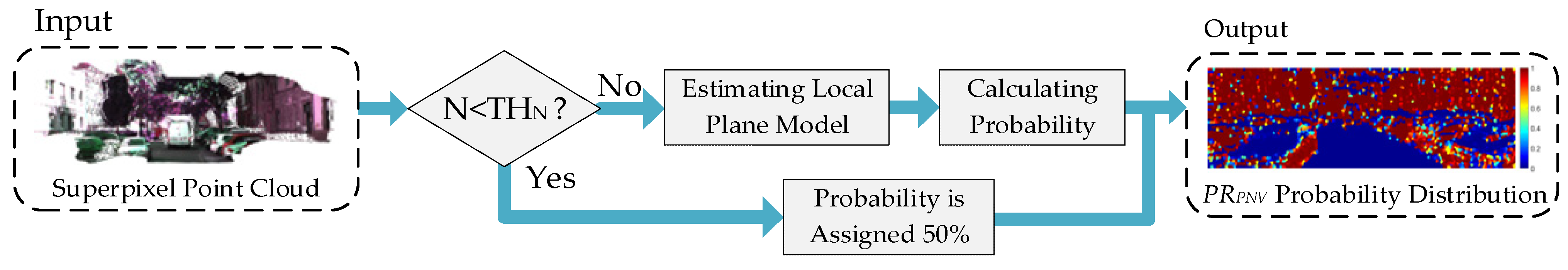
• An Obstacle Detection method based on the Plane Normal Vector (OD-PNV) is proposed. Compared with the traditional obstacle detection method, based on a geometric structure, this method does not need to establish the road surface model, so the detection results are not affected by the road surface fitting accuracy. At the same time, as the method detects each superpixel independently according to its local plane normal vector, it is less affected by conditions such as road surface inclination and unevenness.
• An Obstacle Detection method based on Superpixel Point-cloud Height (OD-SPH) is proposed. This method improves the accuracy of the road plane fitting by combining the results of the OD-PNV method. According to the fitted road plane, the height of the superpixel point cloud from the road surface can be calculated accurately, and obstacles can be detected according to the height value. This method has a good detection effect for the obstacles that protrude obviously from the road surface. It is different from the OD-PNV method in principle and in its feature information, so it plays a very good complementary role to the OD-PNV method.

2. Related Work

Early obstacle detection methods based on stereo vision usually map the depth information into 2D or 3D occupancy grids [15], and locate obstacle regions by finding the occupied grids. As in reference [16], a stochastic occupancy grid was constructed to solve the detection problem of free space area. It applied dynamic programming to the stochastic occupancy grid to finally find the optimal dividing line between the obstacle area and the free space area. However, it could not provide the specific location information of the obstacles. Some references obtain obstacle location information by creating and analyzing a “v-disparity” image. In the “v-disparity” image, roads are projected as approximately horizontal lines, and vertical obstacles are projected as approximately vertical lines. Reference [17] used this principle to detect roads and obstacles, and judged the location of the obstacles by projection difference. This approach reduces the effects of vehicle dynamic pitching. Reference [18] proposed a method that can localize scene elements through sparse 3D point clouds. It first used the “v-disparity” image to detect the depth values of obstacles and extracted the consecutive points corresponding to these depth values from the point cloud. Then, these points were clustered, and finally, the obstacles were located through the clustering results. Although these early methods can detect most obstacles, their detection accuracy is generally low and the amount of information that can be provided is small. Therefore, it is often only suitable for some simple scenes.

From the perspective of vehicle trafficability, traffic scenes can be divided into two classes: obstacle and free space. Free space refers to the part of the road surface that does not contain any obstacle, i.e., the area where the vehicle may enter. In order to segment these two areas, some references first establish a global road surface model, and then detect obstacles by comparing other parts of the scene with the road surface model. For example, reference [19] proposed a road obstacle detection method based on height. The method used point clouds to fit the road plane and calculated the height of the point clouds, and finally detected the obstacles according to the height information of the point clouds. The stixel method, proposed in reference [20], mapped the road surface to a straight line in the v-disparity space, and detected the straight line through Hough transform to determine the road surface model. Then, adjacent rectangular sticks of a certain width and height were used to describe obstacles. Reference [10] proposed the multi-layer stixel on the basis of reference [20]. This method lifted the constraint of the stixel to touch the ground surface and allowed for multiple stixels along every column of the image, thus enabling a more comprehensive description of the traffic scene. Reference [5] proposed an obstacle detection method combining the v-disparity image and stixel method. This method computationally reduced the complexity of making an effective Hough space and improved the accuracy of the road surface extraction results. The digital elevation map method proposed in reference [21] converted the 3D point cloud into a digital elevation map, and combined the quadratic road surface model to detect and represent different types of obstacles. Reference [22] first identified the free space to segment the drivable area, and then used the pixels in the free space to estimate the digital elevation map to improve the estimation accuracy of the road profile. Compared with the original image, the data size of the stixel and digital elevation map is greatly reduced, and the influence of outliers on the detection results is weakened. Therefore, these two scene representation methods are widely used in the current research field of obstacle detection. The road surface models established by the above methods are relatively simple, and they are difficult to fit to the real road surface well. For this reason, some references have introduced more complex road surface profile models, such as clothoid [23] and B-spline surface [24]. However, because the road surface usually presents many local features (such as local protrusions and depressions), it is difficult to use a unified model to describe it. As a result, the detection effect of the above methods largely depends on the accuracy of the road surface parameters and the effectiveness of the models.

Another research idea is to detect obstacle points through the geometric relationship between 3D point pairs. For example, Professor Huang et al. [25] proposed a position-based object segmentation method using the 3D reconstruction capability of stereo vision. This method performed obstacle segmentation based on object depth in an aerial view. Franke et al. [26] analyzed image sequences from the spatial and temporal perspectives. They combined stereo vision and image tracking features to compute 3D point clouds to represent obstacles. In reference [27], instead of using all of the 3D point cloud data, some 3D point cloud candidates extracted by height analysis were used for obstacle detection, which improved the detection accuracy in specific scenes. Reference [28] fused the point cloud of lidar and the image of the camera, obtained the point cloud belonging to the obstacle by using the u-disparity map, and then used the clustering algorithm to segment and locate the obstacles. The images generated by these methods are pixel-level obstacle representations. As there is no need to model the road surface, the detection effect is less affected by the road conditions. Reference [6] proposed a framework of a superpixel-based vehicle detection method using a plane normal vector in the disparity space, which used lane estimation to set the ROI to reduce the amount of calculation. Then, the road plane was fitted by the K-means algorithm, and the candidate areas of the road and obstacles were extracted. Finally, HOG and SVM were used as features and classifiers to verify obstacle candidate areas, respectively. This method took advantage of the geometric relationship between 3D point cloud, but it was still limited by the richness of the data set and the application scenes were limited. However, these methods all need to cluster 3D point clouds. In complex traffic scenes, the uncertainty of the clustering results leads to an unstable detection performance, which is difficult to promote in demanding applications.

In fact, the 3D point clouds contain rich spatial information, and the points in the scene are usually not isolated. The local spatial features of the point cloud can just reflect the connection between the spatial points. Aiming at the complex problem of obstacle detection in traffic scenes, this paper designs an obstacle detection method with a high detection rate and strong stability. This method comprehensively considers the probability of existing obstacles in the local area from the perspective of the plane normal vector feature and superpixel point-cloud height feature. As the spatial information used by these two features is different, the fusion of the two features achieves good results.

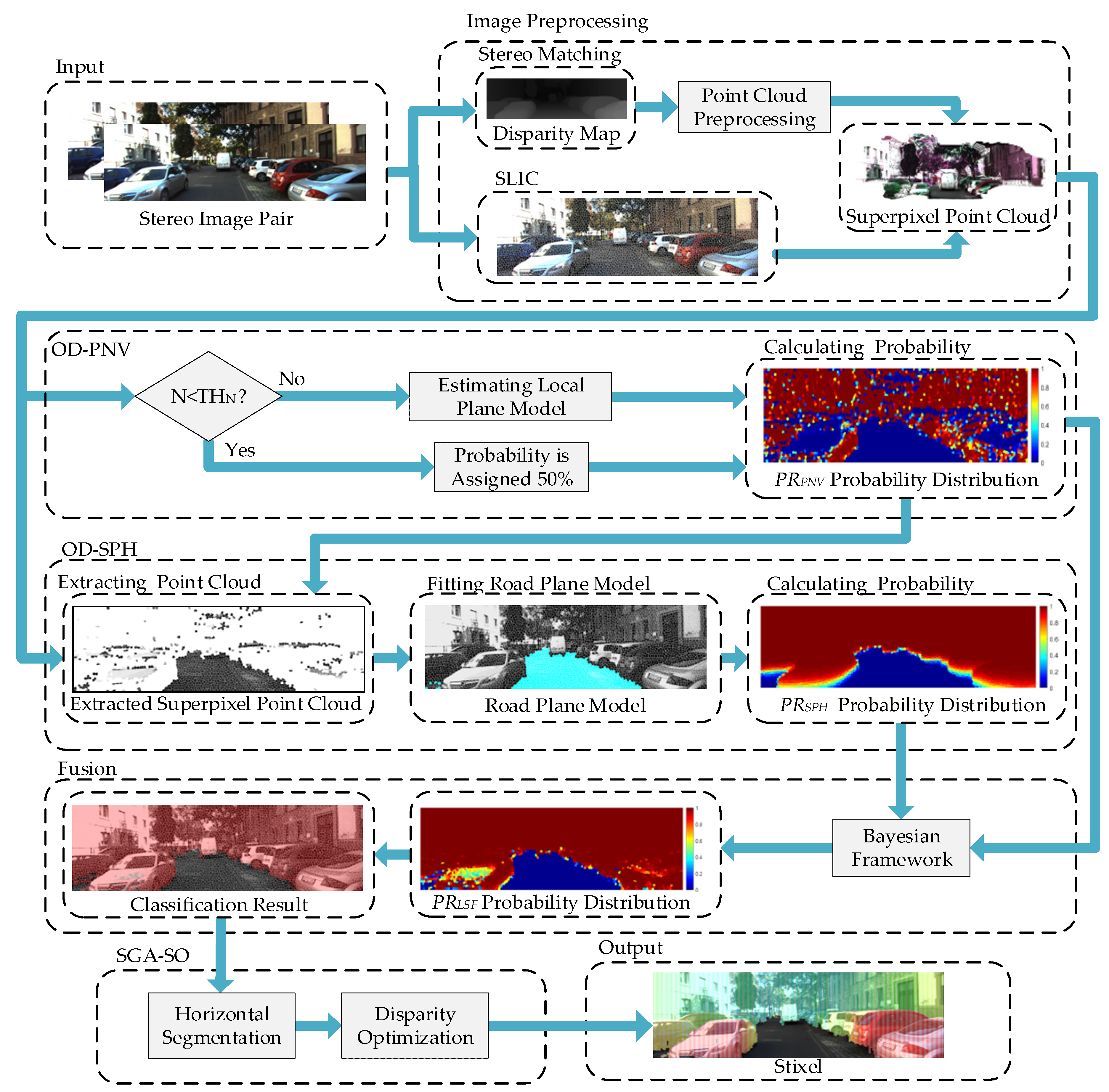
3. Proposed Methods

The flow chart of the proposed obstacle detection method, OD-LSF, is shown in Figure 1. It is mainly divided into Image preprocessing, OD-PNV, OD-SPH, Fusion and a Stixels Generation Algorithm based on Segmentation and Optimization (SGA-SO). Image preprocessing mainly includes stereo matching, superpixel segmentation and point cloud preprocessing. OD-LSF is the main body of this paper, which is mainly composed of four parts; namely, the OD-PNV, OD-SPH, fusion, and Stixels Generation Algorithm based on Segmentation and Optimization (SGA-SO). The OD-PNV method determines the probability that the superpixel belongs to an obstacle by calculating the local plane normal vector according to the fact that the point cloud distribution in the obstacle area tends to be vertical and the point cloud distribution in the free space tends to be horizontal. The superpixels are then classified according to the probability threshold. The larger the distance between the superpixel point cloud and the road surface, the higher the probability that it belongs to the obstacle area. Therefore, the OD-SPH method first determines the road surface by plane fitting the superpixels that are classified as free space by the OD-PNV method, then calculates the height of all the superpixel point clouds from the road surface. Finally, the obtained height information is used to estimate the probability that the superpixel belongs to the obstacle area. The fusion part fuses the probabilities obtained by the OD-PNV and OD-SPH methods, and finally classifies the superpixels according to the fused probabilities. On the basis of the above classification, the SGA-SO algorithm efficiently describes the traffic scene in the form of stixel.

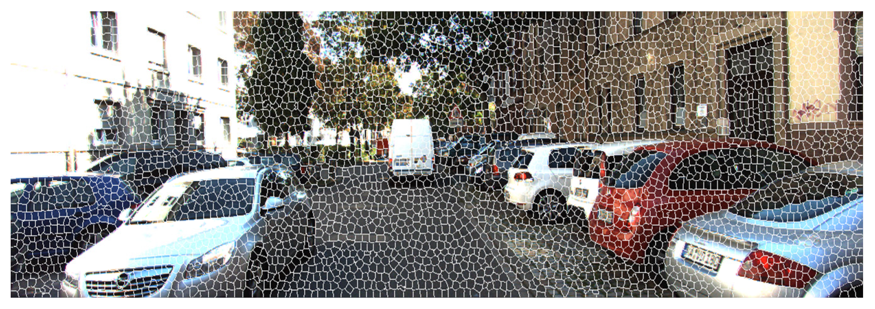
3.1. Image Preprocessing

The OD-LSF method proposed in this paper needs to use the depth information of the pixels, which can be obtained by stereo matching. As stereo matching is not the focus of this paper, we chose the relatively mature algorithm PSMNet [29]. In this paper, a three-dimensional coordinate system is established with the focus of the left camera of the binocular camera as the origin. The specific coordinate (X, Y, Z) of each point in the point cloud in the coordinate system can be obtained by the following calculation formulas:

$$\mathrm{Z}=\frac{B_{line}\ast f}{d}$$

(1)

$$X=\frac{Z\ast \left(x_p-x_{ol}\right)}{f}$$

(2)

$$Y=\frac{Z\ast \left(y_p-y_{ol}\right)}{f}$$

(3)

Among them, $B_{line}$ represents the baseline length of the binocular camera, $f$ represents the focal length of the camera, and $d$ is the disparity. $x_p$ and $y_p$ represent the column coordinate and row coordinate of the pixels in the left image, $x_{ol}$ and $y_{ol}$ represent the column coordinate and row coordinate of the center point of the left image.

The size of the point cloud obtained by stereo matching is usually very large, and it inevitably contains some outliers and invalid value points due to mismatching or distance. Therefore, point cloud filtering [30] is used to preprocess it and improve the quality of the point cloud while reducing the data size. In order to calculate the local spatial feature of the point cloud, this paper adopts the SLIC algorithm [31] to perform superpixel segmentation on the image, and takes the superpixels as the smallest detection unit. The segmentation result of the SLIC algorithm is shown in Figure 2. This algorithm is different from the simple rectangular superpixel segmentation. It can better retain the contour information of the image and make the pixels in the superpixel come from the same object as much as possible. In addition, the SLIC algorithm can reduce the difference in the depth of the point cloud from the same superpixel, which is beneficial to the subsequent plane fitting.

By preprocessing the stereo image, the segmented superpixels and the corresponding point clouds can be obtained. In order to classify the superpixels, this paper proposes two independent methods based on the local spatial features of the point cloud; namely, OD-PNV and OD-SPH. The final probability that each superpixel belongs to an obstacle is obtained by comprehensively considering the outputs of the two methods.

3.2. Obstacle Detection Method Based on Plane Normal Vector (OD-PNV)

The OD-PNV method first performs an initial screening of the input superpixel point clouds to shield the point clouds with too little 3D information. Then, the 3D information of the point clouds contained in the superpixel is used to fit the local plane model. The probability that the superpixel belongs to an obstacle is calculated according to the difference between the normal vector of the local plane model and the normal vector of the free space plane model. The flow chart of the OD-PNV method is shown in Figure 3.

Common obstacles in traffic scenes mainly include vehicles, pedestrians, buildings and vegetation, while free space mainly includes areas such as road and parking lots. Figure 4 shows the point cloud distribution of these two types of objects (the coordinate origin in the figure is the superpixel point cloud centroid, the x-axis coincides with the optical axis and points to the front of the camera, the y-axis is perpendicular to the x-axis and points above the camera, and the z-axis is perpendicular to the y-axis and x-axis and points to the left of the camera). It can be seen from the figure that the point cloud distribution in the obstacle area tends to be vertical, while the point cloud distribution in the free space area tends to be horizontal. If a plane model is used to fit the point cloud in the superpixel, the greater the angle $\theta$ between the normal vector of the plane model and the positive direction of the y-axis, the more the superpixel conforms to the feature of the obstacle area. The OD-PNV method distinguishes the obstacle and the free space by this feature of the point cloud. First, plane fitting is performed on the point cloud in the superpixel; then, the probability that the superpixel belongs to an obstacle is calculated according to the included angle $\theta$.

This method independently calculates the probability that each superpixel belongs to an obstacle based on the plane normal vector. Supposing that $H_o$ shows that the superpixel belongs to an obstacle, and $H_f$ shows the superpixel belongs to a free space, $H_o$ and $H_f$ are mutually exclusive events. Each local plane is represented by model $ax+by+cz+d=0$, then $\overrightarrow{\theta }=(a,b,c)$ represents its normal vector. In order to enhance the robustness of the algorithm, this paper uses the RANSAC algorithm [32] to estimate the local plane model. RANSAC randomly extracts the least original data that satisfy the hypothesis and expands the initial point set with the consistent data points. It is an algorithm to find the optimal model to fit the data through iteration. RANSAC needs to randomly select three points in the point cloud every time, and determine the 3D plane based on these three points. Then, it calculates the distance of each point to the plane, that is, the error. According to the error threshold, it is judged whether each point belongs to the inliers. RANSAC will continue to iterate to find the plane model with the largest number of inliers, that is, the optimal model. The input of the RANSAC algorithm is the 3D point cloud data of the superpixel, and the output is the optimal local plane model parameters and the maximum consistent set. As at least three points are required to determine a plane in 3D space, the minimum subset size of the RANSAC algorithm needs to be set to three. Compared with parameter estimation algorithms, such as least squares estimation, the RANSAC algorithm can more accurately estimate the model parameters from superpixel point clouds containing a large number of outliers.

After obtaining the local plane model parameters of the superpixel, its normal vector $\overrightarrow{\theta }$ can be obtained. Then, the angle $\theta$ between $\overrightarrow{\theta }$ and the positive direction of the y-axis can be expressed as:

$$\theta =\left|\arccos \left(\frac{b}{\sqrt{a^2+b^2+c^2}}\right)\right|.$$

(4)

Among them, $\theta \in \left(0,\pi /2\right)$. In this paper, the Sigmoid function is used to convert $\theta$ into probabilistic form. First, normalize $\theta$ as follows:

$$D{V}_{PNV}=\left(\frac{\theta }{\pi /2}-0.5\right)\ast 10.$$

(5)

Then, the Sigmoid function is built as follows:

$$P{R}_{PNV}=\frac{1}{1+e^{-D{V}_{PNV}}}.$$

(6)

$P{R}_{PNV}$ is approximately between 0 and 1, which is used here to indicate the probability that the superpixel belongs to an obstacle.

Figure 5a shows the probabilistic distribution of an image in the KITTI dataset represented by $P{R}_{PNV}$. The redder the color, the greater the $P{R}_{PNV}$ value, i.e., the higher the probability that the superpixel belongs to an obstacle. In order to classify the superpixel, the decision threshold is set to 0.1, i.e., superpixels with $P{R}_{PNV}>0.1$ are classified as obstacles, otherwise they are classified as free spaces. Figure 5b shows the result after classification. The red area in Figure 5b represents the area classified as an obstacle. As can be seen from the figure, although only a simple threshold segmentation has been conducted, due to the obvious difference between the $P{R}_{PNV}$ values of the two classes, a good classification effect has been achieved. The classification result of the OD-PNV method and the $P{R}_{PNV}$ values obtained in this section will be used in Section 3.3 and Section 3.4, respectively.

As it is difficult for stereo matching to provide accurate depth information for each pixel, the size of the point cloud (the number of points in the point cloud) may be too small in some superpixels. To fit a reliable local plane model, the size of the point cloud must be large enough, so the superpixels with a point cloud too small in size need to be filtered out before fitting. Assuming that the point cloud size of a superpixel is $N$, if $N$ is less than the threshold $T{H}_N$, it is considered that the current superpixel point cloud size is too small to provide a judgment basis for the OD-PNV method, so the probability that the superpixel belongs to an obstacle is set to 0.5.

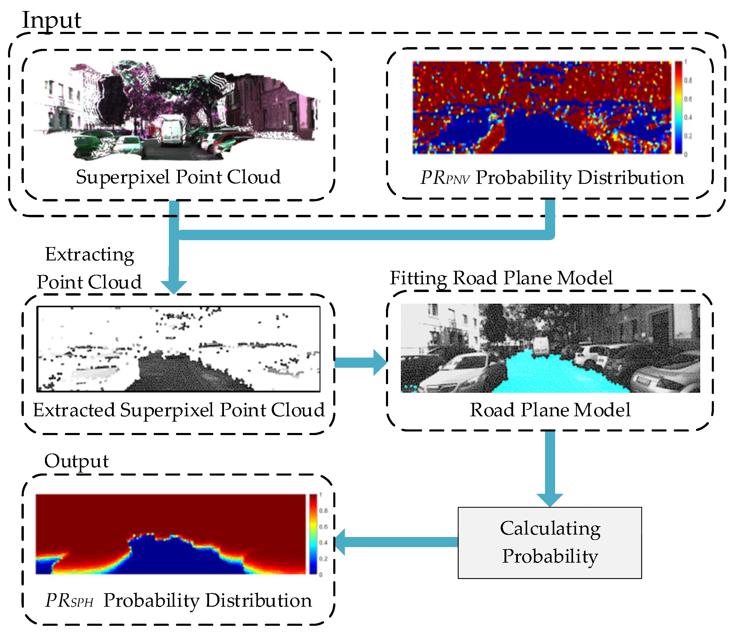
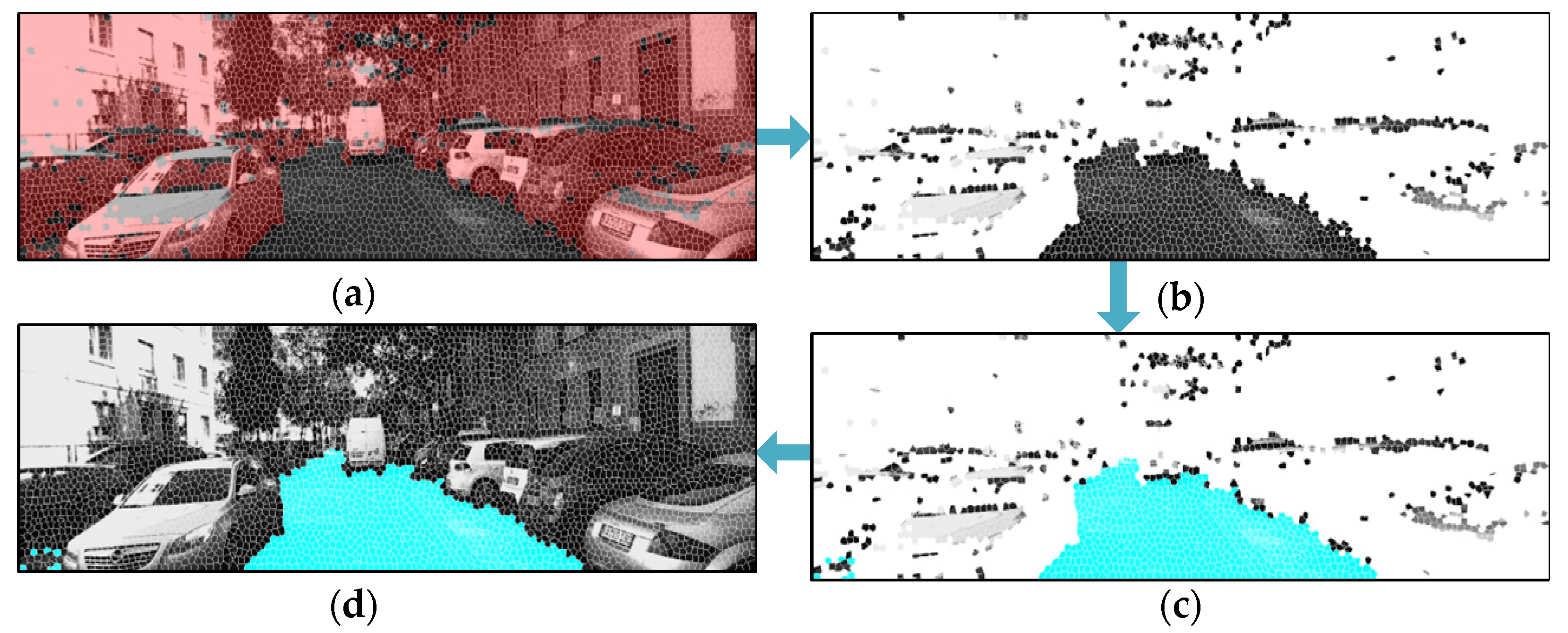
3.3. Obstacle Detection Method Based on Superpixel Point-Cloud Height (OD-SPH)

As mentioned earlier, the OD-PNV method can correctly classify most of the superpixels. However, this method also has certain limitations. It cannot correctly distinguish some obstacle areas with a planar geometry (such as the hood of a vehicle marked by a green box in Figure 5b) from free space areas. Nonetheless, these obstacle areas are usually significantly different in height from the free space areas, and we propose the OD-SPH method based on this difference. The flow chart of this method is shown in Figure 6. To calculate the object height, the road plane model is first estimated by combining the superpixel point cloud information and the classification result of the OD-PNV method. This method calculates the height of the superpixel point cloud based on the estimated model, and then converts the height information into the probability that the superpixel belongs to an obstacle.

If all the superpixel point clouds in the image are used for road plane model fitting, a large part of these superpixels may belong to the obstacle area, which affects the fitting accuracy and efficiency. The OD-SPH method uses the classification result of the OD-PNV method when fitting the model, and its process is shown in Figure 7. First, the superpixel point clouds classified as free spaces by the OD-PNV method are extracted, then the RANSAC algorithm is used to fit the road plane model on these point clouds. As the majority of superpixel point clouds classified as free spaces by the OD-PNV method are located near the road plane, the proportion of inliers in the dataset is significantly increased, thus improving the efficiency of the algorithm. In addition, this method can also avoid false fitting in scenes with complex road conditions.

This paper makes a reasonable assumption based on the obstacle distribution in the traffic scene. That is, the probability of whether a superpixel belongs to an obstacle is related to the height of the point cloud from the road surface. The higher the height of the superpixel point cloud, the greater the probability that it belongs to an obstacle. The height of each point in the superpixel point cloud from the road surface can be calculated according to the fitted road plane model $Ax+By+Cz+D=0$. Assuming that there is a point $p_i\left(x_i,y_i,z_i\right)\left(i=1\dots N\right)$ in the superpixel point cloud, the height of the superpixel point cloud from the road surface can be represented by the mean height $h$ of each point in the point cloud:

$$h=\frac{1}{N}{\displaystyle \sum _{i=1}^N\frac{\left|A{x}_i+B{y}_i+C{z}_i+D\right|}{\sqrt{A^2+B^2+C^2}}}.$$

(7)

Similarly to the OD-PNV method, the Sigmoid function is still used to convert $h$ into a probabilistic form. According to the previous assumption, we set the probability that the superpixels whose height is close to 0 m belong to an obstacle close to 0%. The probability that the superpixels that are close to or exceed $h_m$ (in this paper, $h_m$ is set to 1 m) belong to obstacles is set to be close to 100%. The probability that superpixels with height $h_m/2$ above the ground belong to obstacles is set to 50%. First, normalize the mean height $h$ as follow:

$$D{V}_{SPH}=\left(h-h_m/2\right)\ast 10.$$

(8)

Thus, the Sigmoid function is constructed as follow:

$$P{R}_{SPH}=\frac{1}{1+e^{-D{V}_{SPH}}}.$$

(9)

$P{R}_{SPH}$ is approximately between 0 and 1, which is used here to indicate the probability that the superpixel belongs to an obstacle.

Figure 8 shows the probabilistic distribution of the above image, represented by $P{R}_{SPH}$, and the classification result of the OD-SPH method (the decision threshold is set to 0.15). As can be seen from the figure, as $P{R}_{SPH}$ is obtained from the height of the superpixel point cloud, there is no misjudgment in the obstacle area with a plane geometry, such as the hood of the vehicle. These areas are classified as the obstacle in Figure 8b, and this method makes up for the shortcoming of the OD-PNV method. However, in some areas close to the road surface (such as vehicle tires), the OD-SPH method has the problem of low discrimination, while the OD-PNV method does not have such a problem. Therefore, the fusion of these two methods can achieve complementary effects.

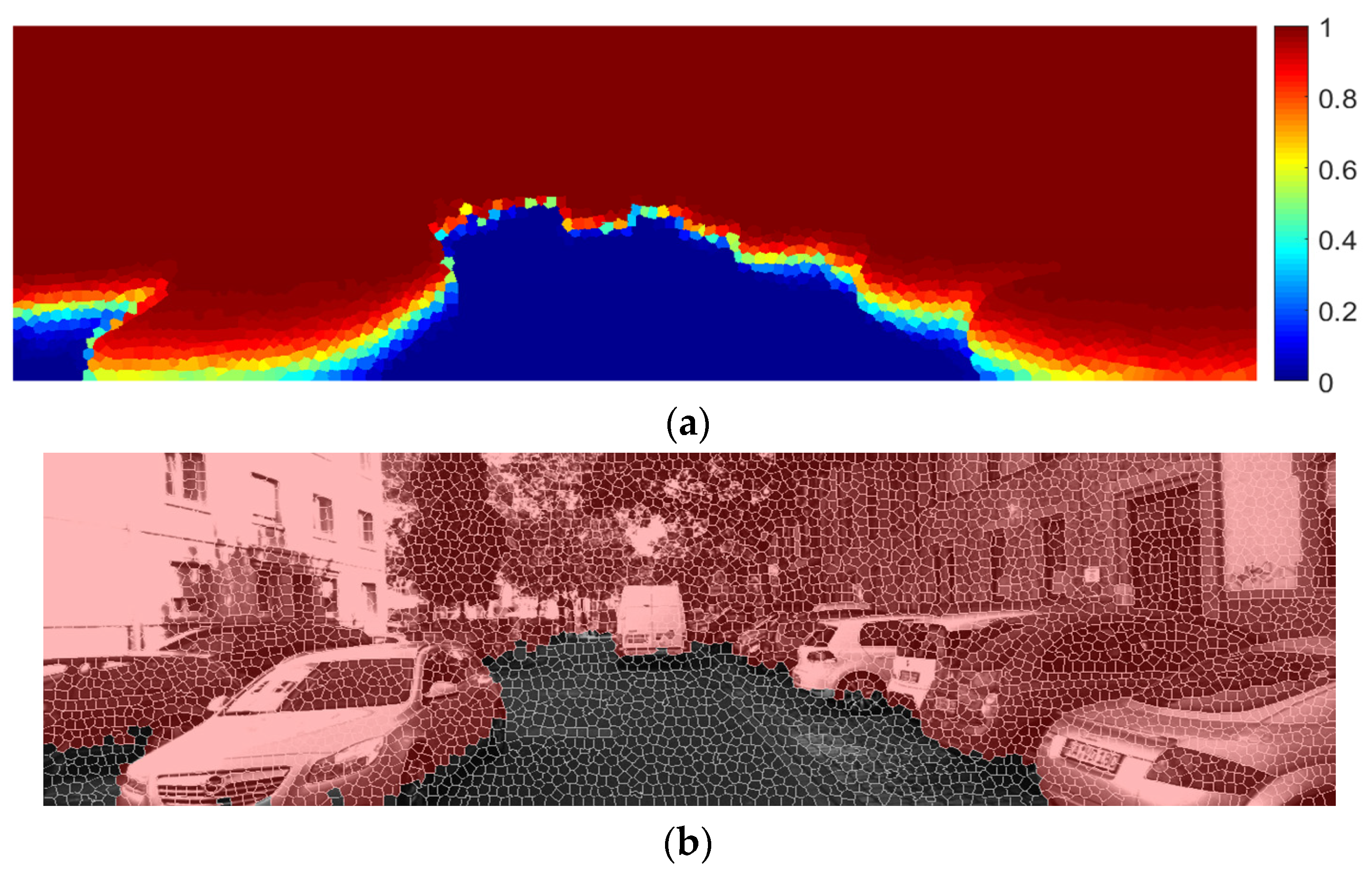
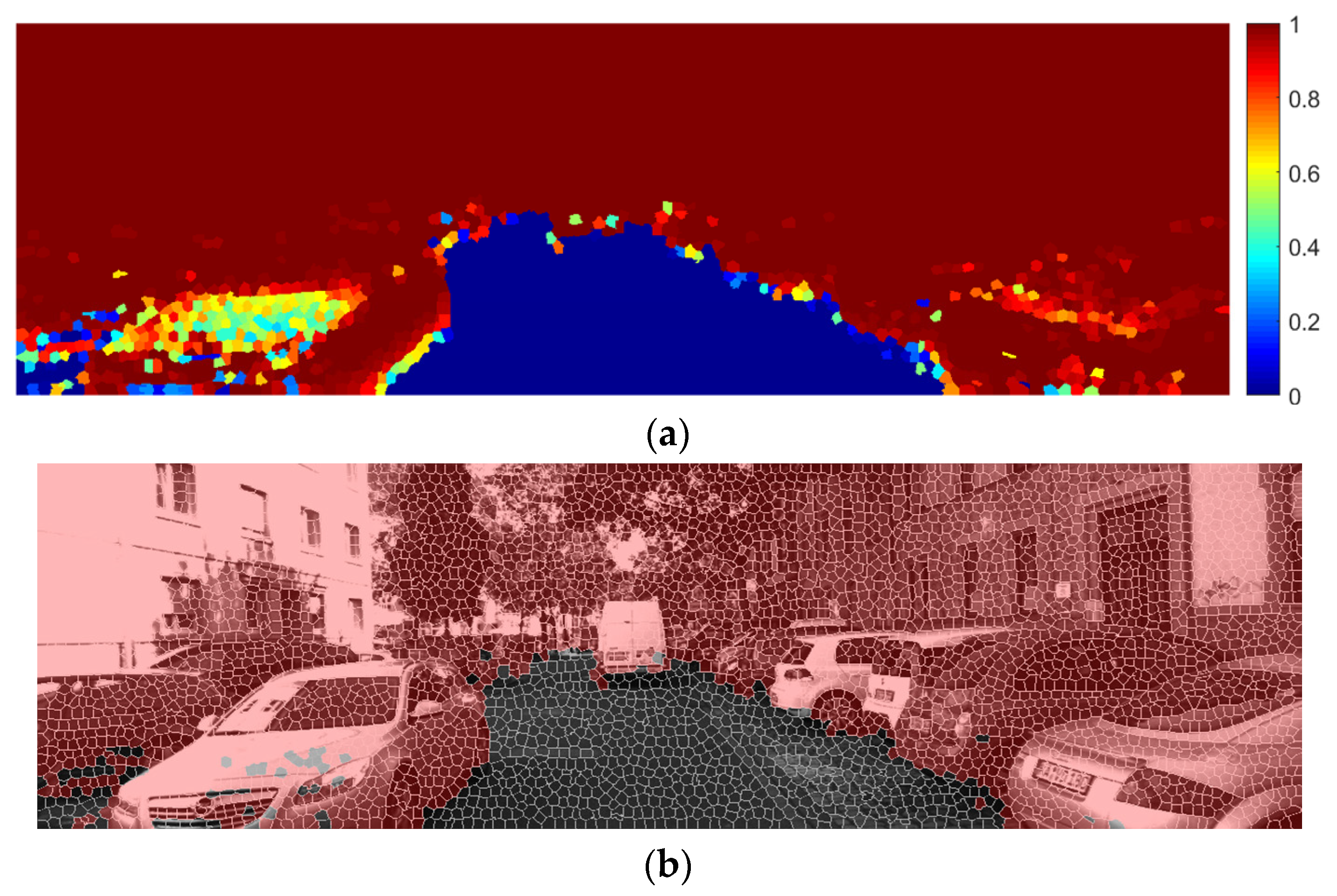
3.4. Probabilistic Fusion

OD-SPH uses the classification results of OD-PNV when fitting the road plane, and its purpose is to better fit the road plane. The probability that the superpixel output by the OD-PNV and OD-SPH methods belongs to an obstacle is only determined by the height and the plane normal vector of the superpixel, respectively. That is, the probability that a superpixel belongs to an obstacle based on the height feature will not be affected by the plane normal vector feature. There is no direct influence between the probability results output by the two methods. The bayesian framework is suitable for decision inference based on the multi-factor probabilistic methods, which is more in line with the human driver’s judgment and decision-making process than the methods of obstacle detection using single information. In order to accurately detect obstacles in complex traffic scenes, this paper proposes the OD-LSF method, which uses the Bayesian framework to fuse the output results of the above two methods to achieve a comprehensive judgment. The probability $P{R}_{LSF}$ that the superpixel belongs to an obstacle is calculated by the following formula:

$$P{R}_{LSF}=\frac{P_{pr}\cdot P{R}_{PNV}\cdot P{R}_{SPH}}{\left(P_{pr}\cdot P{R}_{PNV}\cdot P{R}_{SPH}\right)+\left(1-P_{pr}\right)\left(1-P{R}_{PNV}\right)\left(1-P{R}_{SPH}\right)}.$$

(10)

Among them, $P_{pr}$ represents the prior probability; $P{R}_{PNV}$ and $P{R}_{SPH}$ represent the probability that the superpixel is judged as belonging to an obstacle by OD-PNV and OD-SPH, respectively. Figure 9 shows the probabilistic distribution of the above image represented by $P{R}_{LSF}$ and the classification result of the OD-LSF method (the decision threshold of $P{R}_{LSF}$ is set to 0.45). It can be seen that the OD-LSF method comprehensively considers the output results of the OD-PNV and OD-SPH methods. There is sufficient discrimination in areas such as the hood and tires of the vehicle, and the correct detection results are output.

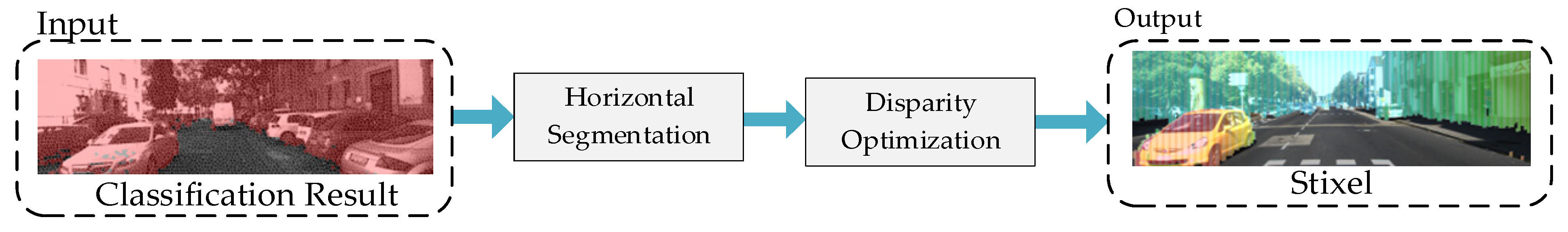
3.5. Stixels Generation Algorithm Based on Segmentation and Optimization (SGA-SO)

Stixels are a superpixel environment description model based on the observation that geometries in an artificial environment are mainly composed of planes. A single stixel is defined as a thin earthbound rectangle with a fixed pixel width and vertical pose [10]. When describing the traffic scene, the stixel shows high accuracy and flexibility, and can compress the output data size, which is particularly suitable for the artificial environment mainly composed of horizontal and vertical structures. In this paper, the stixel includes four attributes: width, base point, top point and depth. The width is the pixel width of the stixel, the base point and the top point mark the beginning and end of each stixel, and the depth represents the distance between the stixel and the camera. On the basis of reference [10], SGA-SO is proposed in this paper. According to the features of the output result of the obstacle detection method proposed in this paper, SGA-SO is divided into two parts: horizontal segmentation and disparity optimization. SGA-SO first performs a column-by-column horizontal segmentation of obstacle superpixels according to a fixed width, and then further optimizes the initially segmented stixels. Figure 10 is the flow chart of SGA-SO.

The input of SGA-SO is the pixel-level classification result of the Fusion output. SGA-SO first horizontally segments the input classification result. It divides the obstacle area according to the width of the stixel, simply divides it into a rectangular image, and then traverses each row of the rectangular image. If there is a pixel point judged to be an obstacle in a row in the rectangular image, it is considered that the row is an obstacle row. Then, divide the obstacle row and the adjacent obstacle row into the same stixel. The specific horizontal segmentation process is shown in Algorithm 1.

Algorithm 1. Horizontal Segmentation

Input:$input\_img$: Pixel-level label image of classification result; $width$: Stixel width; $input\_img.row$: The number of rows of the input image; $input\_img.col$: The number of columns of the input image; $input\_img.extract\left(a,b\right)$: Extract column $a$ to column $b$ of $result\_img$ and return Mat type data; $block$: Segmented rectangular image; $block.row\_data(i)$: The function is to return the data of row $i$ in $block$; $judge\left(block.row\_data(i)\right)$: The function is to judge whether there is a pixel judged as an obstacle in row $i$, and return 0 if it exists, otherwise return 1 Output: $S$: List of $stixel$

$width=5$, $f=0$, $f\_last=0$, $k=0$ $N=input\_img.col/width$ while $k<N$ do  $block$=$input\_img.extract\left(k\ast width,\left(k+1\right)\ast width\right)$, $f=0$, $f\_last=0$   while $i<input\_img.row$ do       $f=judge\left(block.row\_data(i)\right)$    if$f==0$and$f\_last==1$     $S.push\left(stixel\right)$, $stixel.clear()$     $stixel.push\left(block.row\_data\left(i\right)\right)$    else if$f==0$and$f\_last==0$     $stixel.push\left(block.row\_data\left(i\right)\right)$    end if    $f\_last=f$, $i++$   end while  $k++$ end while

The superpixels detected as obstacles are horizontally segmented according to the fixed stixel width. The segmented stixels are shown in Figure 11a, where the width of the stixel is 5 pixels. The depth value of the stixel is the average depth of the pixels it contains, and the redder its color is, the closer it is to the camera. Following the horizontal segmentation, obstacles with great differences in their depth may still be divided into the same stixel, such as the cars and buildings marked by a black box in Figure 11a.

In order to enable a stixel to better describe the obstacle, disparity optimization is further performed on the horizontally segmented stixels to obtain multi-layer stixels. The optimization process is as follows: each row of the stixel is traversed from top to bottom, and the mean disparity of the current row is calculated. Determine whether the difference between the mean disparity of the current row and the previous row is within the disparity optimization threshold. The stixel is truncated if the difference exceeds the disparity optimization threshold. The optimized stixels are shown in Figure 11b, where the disparity optimization threshold is five. It can be seen from the figure that the optimized stixels are truncated between two cars and between cars and buildings, and the area covered by the same stixel is basically the same obstacle, as shown in the black box in Figure 11b. In addition, the color of the optimized stixels also reflects the distance of different obstacles. Therefore, the optimized stixels can more accurately describe the traffic scenes, which are conducive to deepening the understanding of the scenes. The specific disparity optimization process is shown in Algorithm 2.

Algorithm 2. Disparity Optimization

Input:$S$: List of $stixel$; $N$: Number of $stixel$; $i$: Number of current row in $stixel$; $S[\cdot ].\max \_row$: The maximum number of rows in the current $stixel$; $S[\cdot ].\min \_row$: The minimum number of rows in the current $stixel$; $mean(stixel,i)$: The function to calculate mean depth of row $i$ in input $stixel$; $truncate(stixel,i)$: The function truncate $stixel$ at row $i$, generates and returns new $stixel$ Output: $S\_opted$: list of optimized $stixel$

$i=0$, $k=0$, $dep=0$, $dep\_last=0$, $S\_opted=[]$, $TH=5$ while $k<N$ do while $i<=(S[k].\max \_row-S[k].\min \_row)$ do   $dep=mean(S[k],i)$   if$(dep-dep\_last)>TH$    $S\_opted.push(truncate(S[k],i))$   else if$i+S[k].\min \_row==S[k].\max \_row$  $S\_opted.push(truncate(S[k],i))$  end if  $dep\_last=dep$, $i++$  end while $k++$ end while

4. Experiment and Result Analysis

4.1. Experimental Environment and Parameter Settings

The experiment is based on OpenCV and PCL, the programming language is C++, and the experiment is implemented in the windows operating system. In terms of the experimental hardware, the CPU is AMD Ryzen5 5600U. Its frequency is 2.30 GHz, and the memory space is 16 GB. The width of the stixel is 5 pixels and the thresholds of $P{R}_{PNV}$, $P{R}_{SPH}$ and $P{R}_{LSF}$ are set to 0.1, 0.15 and 0.45, respectively. The above parameters are the optimal parameters obtained during the experiment. There are also some parameters that have little influence on the experimental result, so we empirically selected an appropriate threshold; for example, the error threshold for determining inliers/outliers in RANSAC is set to 0.1, the prior probability $P_{pr}$ is 0.5, and the disparity optimization threshold is set to 5. All of the methods in the experiment use the same disparity data.

The specific implementation process of the OD-LSF method is as follows: first input the stereo image pair in the data set, calculate the disparity map, and further calculate the point cloud information, and generate the superpixel point cloud through the segmentation result of the SLIC algorithm and the point cloud information. In the second step, the superpixel point cloud information is input into the OD-PNV method, and the probability that the superpixel belongs to an obstacle is calculated through the local plane normal vector feature. In the third step, the detection results of the OD-PNV method and the superpixel point cloud are input into OD-SPH, and the road plane is fitted to obtain the local height features. The OD-SPH method calculates the probability that the superpixel belongs to an obstacle through the local height feature. In the fourth step, the detection results of the two methods are fused using the Bayesian framework. Finally, SGA-SO is used to generate the stixel and output obstacle detection result.

4.1.1. Baseline

In order to compare the performance differences between different detection methods, the OD-LSF method is compared with the following four methods: (1) Reference [19]: It is a new method, recently proposed, which can calculate the probability that a superpixel point cloud belongs to an obstacle according to its height from the road surface, and complete the obstacle detection in traffic scenes; (2) Reference [10]: It is a classic obstacle detection method based on stereo vision that can describe the traffic scenes using a multi-layer stixel; (3) The OD-PNV method proposed in this paper; (4) The OD-SPH method proposed in this paper. For the convenience of comparison, the outputs of reference [19], the OD-PNV method and the OD-SPH method are represented in the form of a stixel using the SGA-SO proposed in this paper. The detection performance of the methods based on the obstacle height can be evaluated by comparing reference [19] with the OD-SPH method, and the detection performance of the fusion methods can be evaluated by comparing OD-LSF with OD-PNV and OD-SPH.

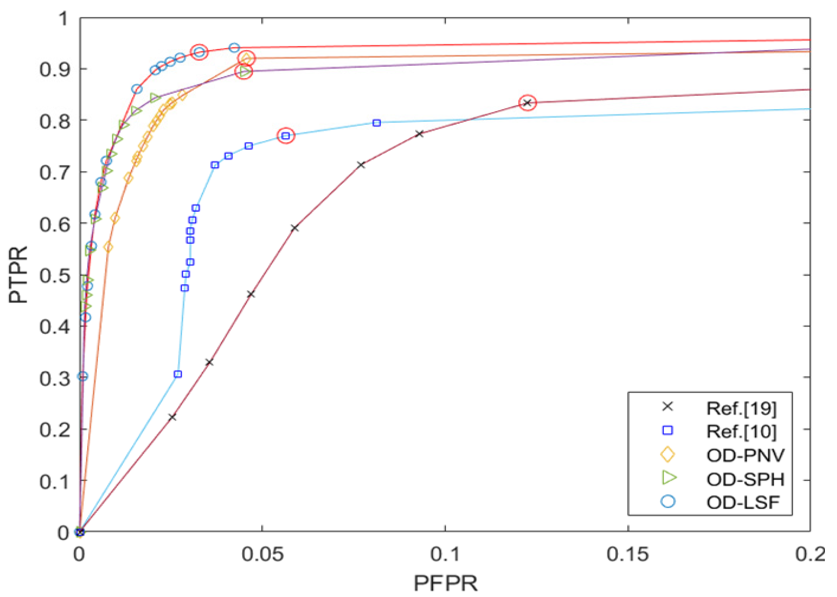
4.1.2. Evaluation Criteria

For the detection task, the Pixel-wise True Positive Rate (PTPR) and Pixel-wise False Positive Rate (PFPR) are two important indicators, which reflect the coverage and judgment ability of the detection method to the object, respectively. Therefore, the above two pixel-wise evaluation indicators are used as quantitative performance evaluation criteria in this paper. PTPR can be expressed as follows:

$$PTPR=\frac{TP}{TP+FN}.$$

(11)

Among them, $TP$ is the number of pixels correctly detected as obstacles; $TP+FN$ is the pixel number of real obstacles. PFPR can be expressed as follows:

$$PFPR=\frac{FP}{FP+TN}.$$

(12)

Among them, $FP$ is the number of pixels falsely detected as obstacles; $FP+TN$ is the pixel number of real free spaces.

In addition, the Receiver Operating Characteristic (ROC) curve is used to determine the optimal parameters of each detection method. The abscissa of the ROC curve is PFPR, and the ordinate is PTPR. By executing the detection method under different parameters, the detection results are mapped to a series of points in the plane, and the optimal parameters are determined according to the convex hull positions of the ROC curves.

4.1.3. Dataset

The semantic segmentation dataset of KITTI [33] is selected as the experimental dataset. This dataset has abundant images of urban traffic scenes, including a variety of obstacle types, and the corresponding semantic annotations are provided. The KITTI semantic dataset does not give the label of the test set, but only the label of the training set, so this experiment only uses the training set and divides it again. There are 200 images in the training set of the KITTI semantic dataset, 100 images of which are randomly selected as the training set for this experiment, and the other 100 images are used as the test set. The training set is used to draw the ROC curve and select the optimal parameters, and the test set is used to test the performance of each method under the optimal parameters.

The semantic segmentation dataset of KITTI divides the pixels in the image into various classes according to the common objects in the traffic scene. However, as this paper only focuses on the obstacles and free spaces in the traffic scenes, the pedestrians, vehicles, buildings, and vegetation are classified into the obstacle class, while the roads, sidewalks and parking lots are classified into the free space class. Among the pixel classes defined in the dataset, the sky class and nature-terrain class are ignored in this paper. This is because the disparity of the sky is difficult to measure accurately, and the position of the sky has almost no effect on vehicle driving. Some nature-terrain is on the same plane as the road surface, while others are much higher than the road surface, so it is difficult to define whether the nature-terrain is free space or an obstacle. We performed a statistical analysis of the pixel number with different obstacle class labels in the dataset. The statistical result indicates that the pixel number of obstacle classes closely related to traffic behavior, such as vehicles, pedestrians and traffic signs, only account for 9.02% of the total pixel number, while the pixel number of obstacle classes far from the vehicle, such as buildings and vegetations, account for 50.71% of the total pixel number. Although the former accounts for a relatively small proportion, they are obviously more worthy of attention. If the two are not distinguished, the optimal parameters obtained from the ROC curves are mainly determined by obstacles such as buildings and vegetation. In order to make the algorithm pay more attention to obstacles such as vehicles, pedestrians and traffic signs, this paper divides a key obstacle subclass in the obstacle class and draws ROC curves with the key obstacle subclass of the training set to obtain the optimal parameters. In the quantitative evaluation of the performance of each method, the obstacles in the test set are, respectively, evaluated according to the key obstacle subclass and the complete obstacle class. In the following experiment, the key obstacle subclass includes pedestrians, vehicles and traffic signs, while buildings, trees, sky and nature-terrain are ignored. The complete obstacle class includes pedestrians, vehicles, traffic signs, buildings and trees, ignoring sky and nature-terrain.

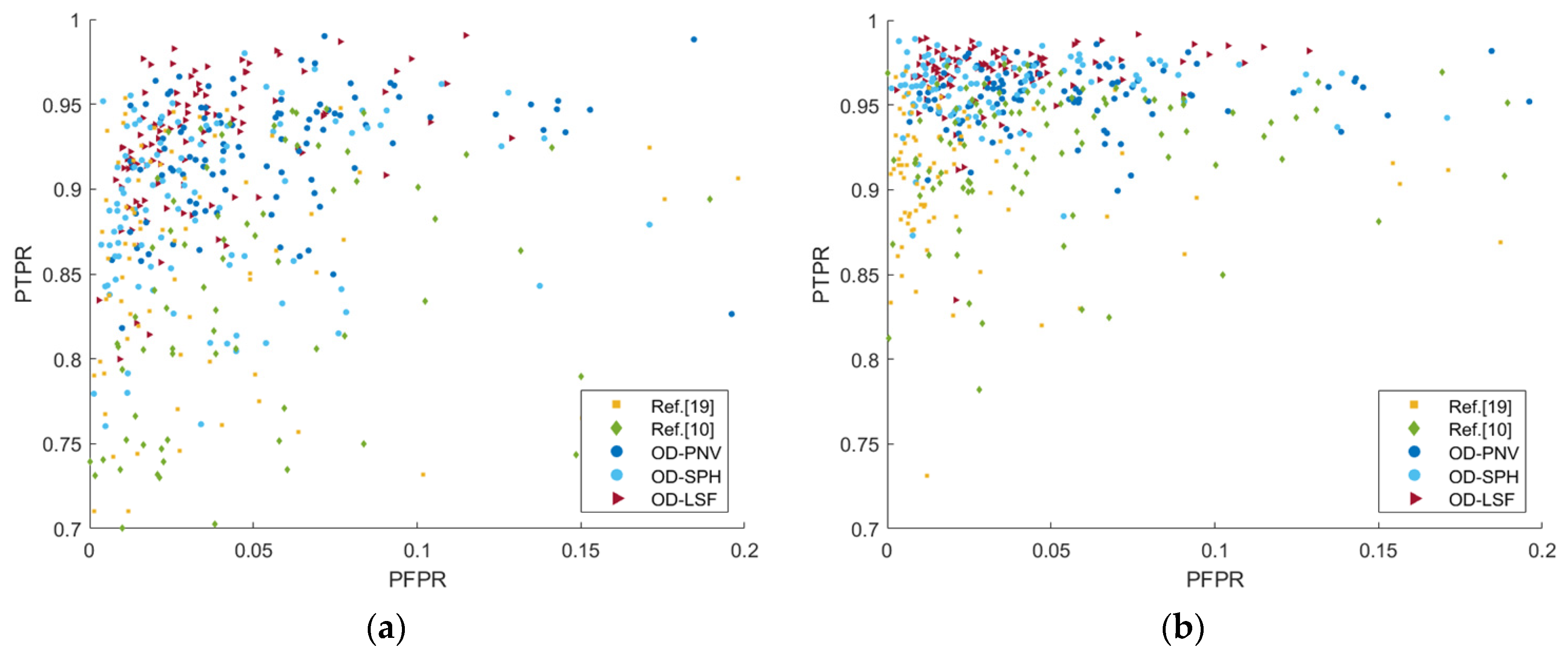
4.2. Quantitative Analysis

In order to determine the optimal parameters of each detection method, the ROC curves of the above five methods are plotted based on the key obstacle subclass in the training set, as shown in Figure 12. Among them, the main parameters of reference [19] are the obstacle probability threshold. The main parameters of reference [10] are the vertical cut costs used in dynamic programming and the width of the stixels. The main parameters of the OD-PNV, OD-SPH and OD-LSF methods are the width of the stixels and the obstacle probability threshold. The optimal parameters are selected according to the convex hull position of each curve (as shown by the red circle in Figure 12).

The detection performance indicators of the five methods in the test set under the optimal parameters are shown in

Table 1. Detection performance indicators of the five methods.

	Key Obstacle Subclass		Complete Obstacle Class
Method	PTPR(%)	PFPR(%)	PTPR(%)	PFPR(%)
Ref. [19]	83.3	12.2	89.4	12.2
Ref. [10]	76.9	5.6	88.6	5.6
OD-PNV	92.2	5.5	95.4	5.5
OD-SPH	88.9	3.8	96.0	3.8
OD-LSF	92.7	3.5	96.8	3.5

. By comparing Figure 12 and Table 1, it can be found that the ranking of the five methods according to the performance indicators is completely consistent in the training set and the test set. Table 1 indicates that the three methods proposed in this paper, OD-PNV, OD-SPH and OD-LSF, are superior to the other two methods in terms of the PTPR and PFPR, while OD-LSF achieves the highest PTPR and lowest PFPR, respectively. The indicators of the OD-SPH and OD-LSF methods in the detection of a complete obstacle class are relatively close. This is because the OD-SPH method is good at detecting obstacles in higher spaces, such as buildings and vegetation, which account for a large number of pixels. In the detection of a key obstacle subclass, the PTPR indicator of the OD-LSF method is significantly better than that of the OD-SPH method, which indicates that the fusion of the two local spatial features improves the detection ability of the OD-LSF method for the key obstacle subclass. The PFPR indicator of the OD-LSF method is obviously superior to the OD-PNV method, which is because the OD-LSF method incorporates the height information of obstacles and corrects the false detection of the OD-PNV method to a certain extent. Reference [19] and the OD-SPH method are relatively close in principle, as both rely on height information to detect obstacles, but the performance indicators of the OD-SPH method are better than reference [19]. This is because the OD-SPH method uses the classification result of the OD-PNV method in its road surface model fitting, which avoids false fitting in scenes with a complex road surface. In some complex traffic scenes, reference [19] relies solely on the height information of the 3D points, so it is possible to fit the false road surface model, which will have a significant impact on the performance indicators.

Figure 13 shows the PTPR over PFPR scatter plots of the five methods under the two obstacle classification standards. A high PTPR and low PFPR (upper left corner of the figure) can reflect the best detection performance. It can be seen from the figure that the points of the OD-LSF method under the two obstacle classification standards are closer to the upper left corner of the figure than the other four methods, and the distribution of the points is more concentrated. This indicates that the OD-LSF method not only performs better in terms of its detection performance, but also is stronger than the other methods in terms of its stability.

In terms of operating efficiency, the average single-frame running time of reference [19], reference [10], OD-PNV, OD-SPH, and OD-LSF are 203 ms, 175 ms, 209 ms, 214 ms, and 223 ms, respectively. The average single-frame running time of the above methods are all obtained in the same experimental environment. It can be seen that the average single-frame running time of the five methods are almost the same, all approximately 200 ms. The operating efficiency of the method is closely related to the experimental environment. In a better hardware environment, the methods we propose will perform better.

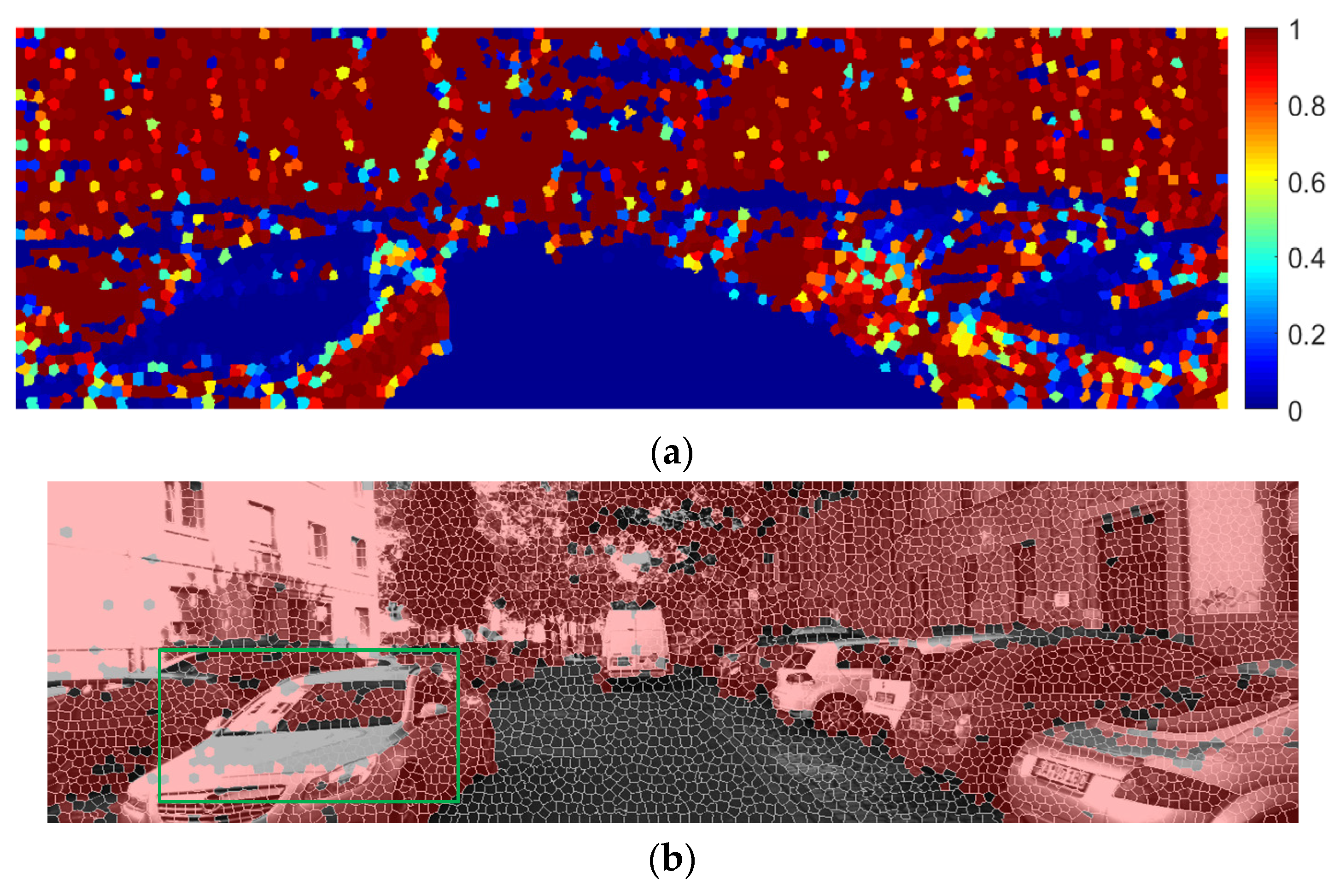
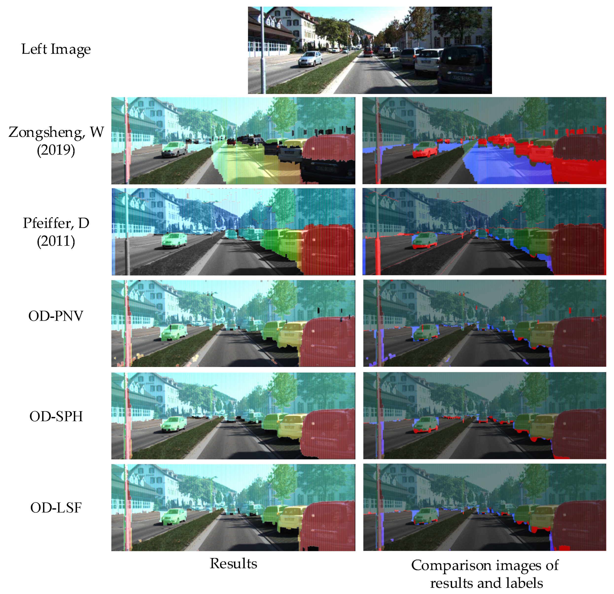
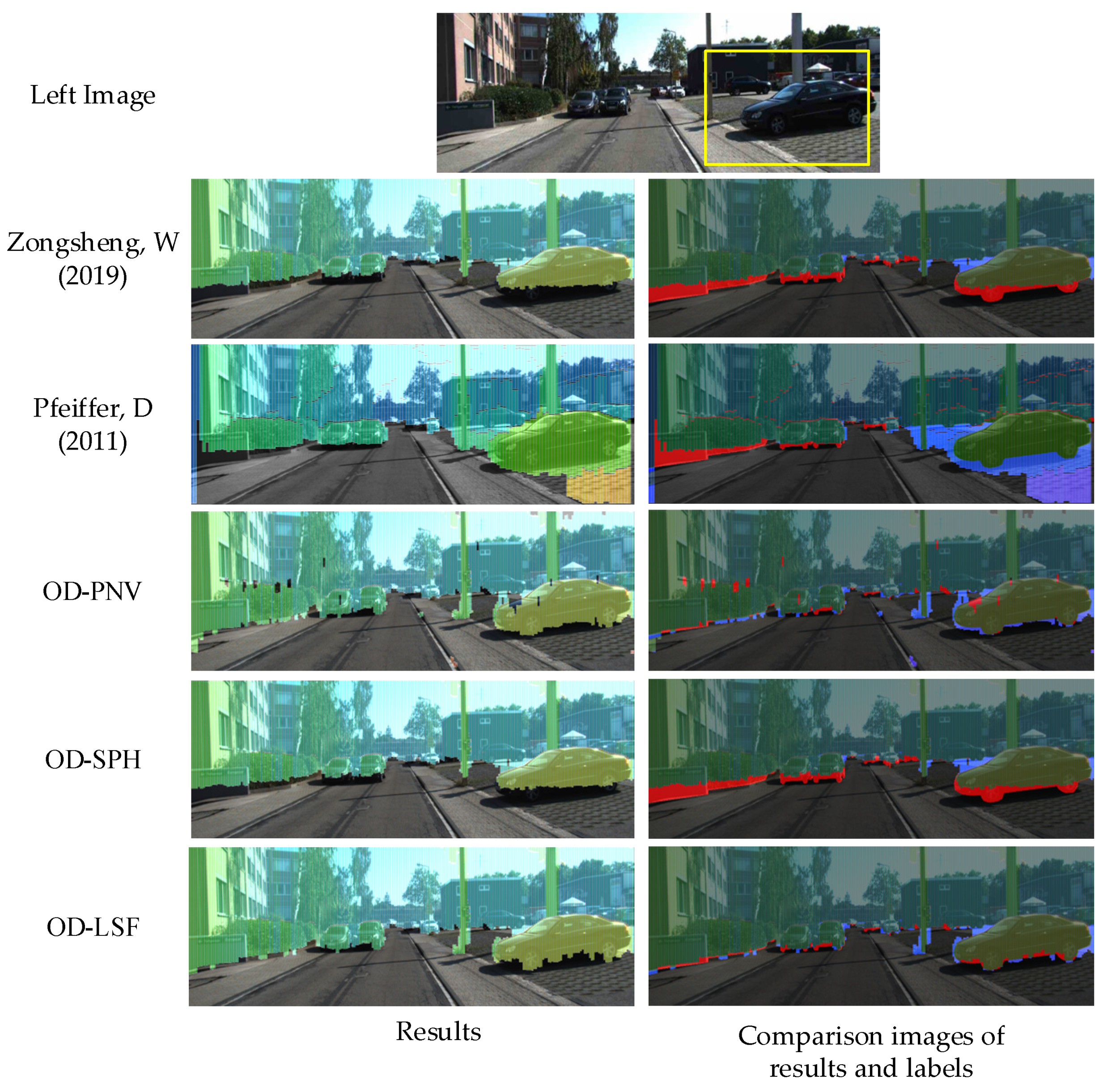
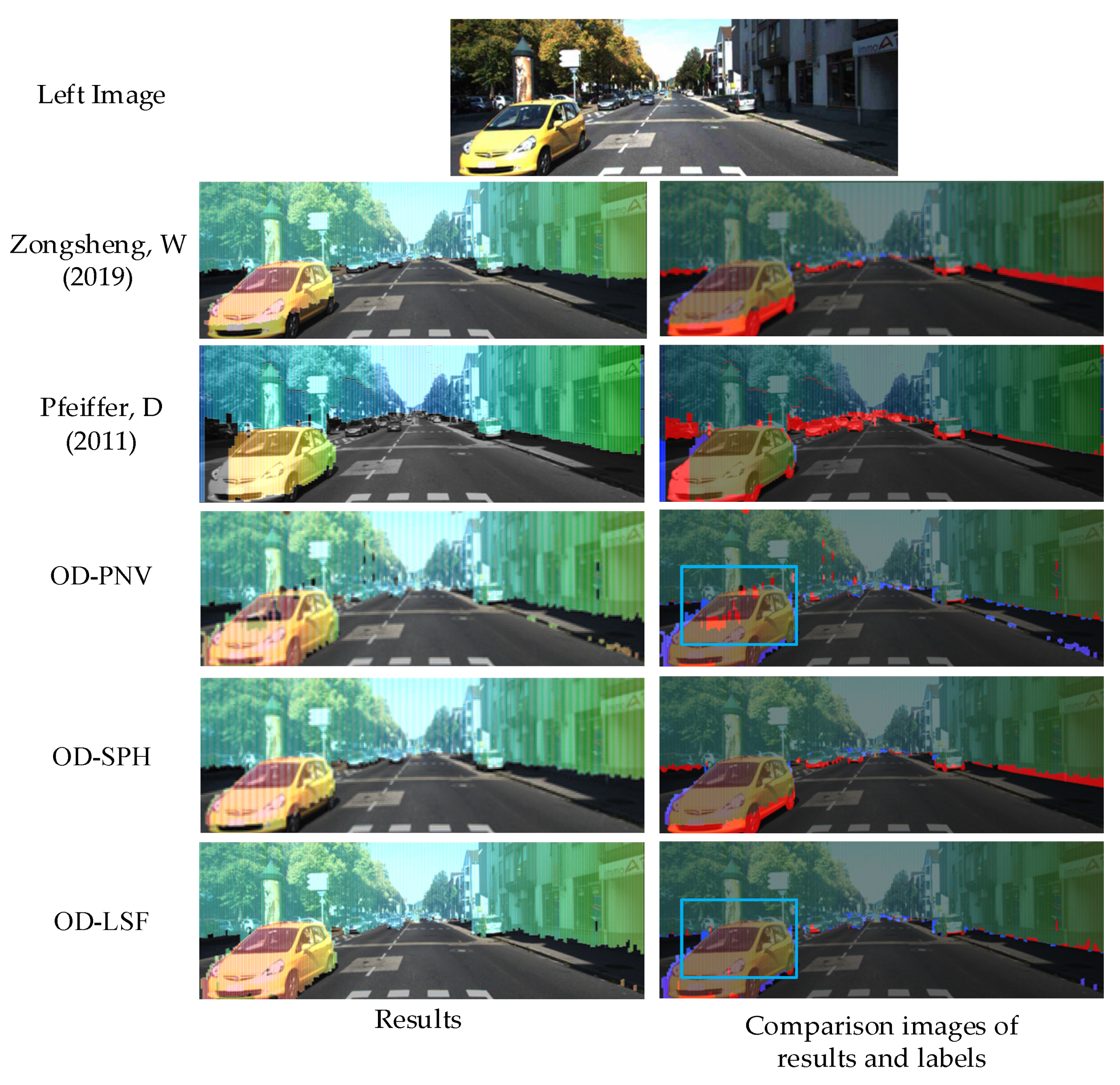
4.3. Qualitative Analysis

In order to qualitatively analyze the performance of the five methods in the KITTI dataset, three scenes are selected as examples. Figure 14, Figure 15 and Figure 16 are the detection results of the five methods in scene 1, scene 2 and scene 3, respectively. The first row is the left image of the binocular images, and the first column of Figure 14, Figure 15 and Figure 16 is the detection results of the five methods. The redder the color of the stixel, the closer the distance. In order to show the detection effect more clearly, comparison images between the detection results and the labels are further drawn. As shown in the second column of Figure 14, Figure 15 and Figure 16, the highlighted areas are the error detection areas, the red areas are the areas where the obstacles are misclassified as free spaces, and the blue areas are the areas where the free spaces are misclassified as obstacles.

It can be seen from Figure 14 and Figure 15 that there are two planes with different heights, the lawn and the road, in scene 1, and the horizontal road plane and the parking lot area with a certain inclination relative to the road plane appear in scene 2 (the area indicated by the yellow box in the left image). These two scenes are common uneven road scenes in urban road environments. In scene 1, reference [19] judged a large part of the free space as an obstacle, and there is an obvious misdetection. In scene 2, reference [10] misdetects most of the road surface of the parking lot as obstacles. The above situation occurs because these two methods rely on the accuracy of the road surface model, and if the road surface model cannot match the actual situation, it will have a negative impact on the detection performance. The OD-SPH method proposed in this paper also relies on an accurate road surface model, but it uses superpixel point clouds classified as free space by the OD-PNV method for road surface fitting. Therefore, the accuracy of the road surface fitting is improved, and the above-mentioned false detection situation is avoided. The false detection areas of OD-PNV are mainly concentrated near the hood of the vehicle, which does not consider the superpixel height feature, and is less affected by the uneven road surface. OD-LSF considers two kinds of spatial features comprehensively, and the false detection caused by the height feature error can be compensated by the plane normal vector feature. Therefore, the impact of an uneven road on OD-LSF is limited, and its detection results are the best in scene 1 and scene 2.

Scene 3, shown in Figure 16, is a typical flat road scene in urban scenes. It can be seen from the figures that both reference [19] and the OD-SPH method detect obstacles close to the road as free space. This shows that even if the road model can correctly match the actual situation, it is difficult for these methods, which only rely on height features to correctly detect obstacles that are closer to the road surface. The false detection areas of the two methods of OD-PNV and OD-LSF are significantly smaller than that of the other three methods. However, it can be seen from the figure that the OD-PNV method has relatively more false detections in the hood and roof of the yellow vehicle (the area shown in the blue box in the figure). This is mainly because the area and the road surface have similar local plane normal vector features, so it is difficult to accurately distinguish them by only relying on the plane normal vector feature. The OD-LSF method makes up for the false detection caused by the plane normal vector feature through the height feature.

The OD-LSF method proposed in this paper combines the advantages of the OD-PNV and OD-SPH methods. The detection effect has been significantly improved in the obstacle area close to the road surface and the vehicle hood and roof, and it can adapt to some uneven road scenes.

5. Conclusions

In order to improve the environment perception ability of the ADAS, the new obstacle detection method based on the local spatial feature (OD-LSF) is proposed in this paper. Firstly, an obstacle detection method based on the plane normal vector (OD-PNV) is proposed. This method classifies the superpixels as obstacles or free spaces based on the superpixel local plane normal vector. It does not need to fit a road surface model, so it is less affected by the road condition. In addition, an obstacle detection method based on the superpixel point-cloud height (OD-SPH) is proposed. This method uses the superpixels classified as free spaces by the OD-PNV method to fit the road plane and classify them according to the superpixel point-cloud height. Finally, the OD-LSF method combines the detection probabilities provided by the above two methods, and the results show that the OD-LSF method combines the advantages of the two methods. The experiment on the KITTI dataset indicates that the OD-LSF method proposed in this paper combines the advantages of the above two methods. For the detection of the complete obstacle class and key obstacle subclass, the PTPR is 96.8% and 92.7%, respectively, and the PFPR is 3.5% for both. Even in the uneven road environment, our method achieves good detection results. However, the experimental results also indicate that the OD-LSF method has a limited detection capability for irregular vegetation covered areas. In our future work, we will study how to expand the detection range of the OD-LSF method. At the same time, optimizing the algorithm structure of OD-LSF and improving the operation efficiency are also our future work.

References

- World Health Organization. Global Status Report on Road Safety 2018: Summary (No. WHO/NMH/NVI/18.20); World Health Organization: Geneva, Switzerland, 2018. [Google Scholar]
- Orlovska, J.; Novakazi, F.; Lars-Ola, B.; Karlsson, M.; Wickman, C.; Söderberg, R. Effects of the driving context on the usage of Automated Driver Assistance Systems (ADAS)-Naturalistic Driving Study for ADAS evaluation. Transp. Res. Interdiscip. Perspect. 2020, 4, 100093. [Google Scholar] [CrossRef]
- Yu, X.; Marinov, M. A study on recent developments and issues with obstacle detection systems for automated vehicles. Sustainability 2020, 12, 3281. [Google Scholar] [CrossRef]
- Yeong, D.J.; Velasco-Hernandez, G.; Barry, J.; Walsh, J. Sensor and Sensor Fusion Technology in Autonomous Vehicles: A Review. Sensors 2021, 21, 2140. [Google Scholar] [CrossRef] [PubMed]
- Luo, G.; Chen, X.; Lin, W.; Dai, J.; Liang, P.; Zhang, C. An Obstacle Detection Algorithm Suitable for Complex Traffic Environment. World Electr. Veh. J. 2022, 13, 69. [Google Scholar] [CrossRef]
- Seo, J.; Sohn, K. Superpixel-based Vehicle Detection using Plane Normal Vector in Dispar ity Space. J. Korea Multimed. Soc. 2016, 19, 1003–1013. [Google Scholar] [CrossRef]
- Royo, S.; Ballesta-Garcia, M. An Overview of Lidar Imaging Systems for Autonomous Vehicles. Appl. Sci. 2019, 9, 4093. [Google Scholar] [CrossRef]
- Lee, Y.; Park, S. A Deep Learning-Based Perception Algorithm Using 3D LiDAR for Autonomous Driving: Simultaneous Segmentation and Detection Network (SSADNet). Appl. Sci. 2020, 10, 4486. [Google Scholar] [CrossRef]
- Peilin, L.; Cuiqun, H.; Zhichun, L. Comparison and analysis of eye-orientation methods in driver fatigue detection. For. Eng. 2008, 24, 35–38. [Google Scholar]
- Pfeiffer, D.; Franke, U. Towards a global optimal multi-Layer stixel representation of dense 3D data. In Proceedings of the 22nd British Machine Vision Conference(BMVC), Dundee, UK, 29 August–2 September 2011; pp. 1–12. [Google Scholar]
- Pinggera, P.; Ramos, S.; Gehrig, S.; Franke, U.; Rother, C.; Mester, R. Lost and found: Detecting small road hazards for self-driving vehicles. In Proceedings of the 2016 IEEE/RSJ International Conference on Intelligent Robots and Systems (IROS), Daejeon, Republic of Korea, 9–14 October 2016; pp. 1099–1106. [Google Scholar]
- Alzubaidi, L.; Zhang, J.; Humaidi, A.J.; Al-Dujaili, A.; Duan, Y.; Al-Shamma, O.; Santamaría, J.; Fadhel, M.A.; Al-Amidie, M.; Farhan, L. Review of deep learning: Concepts, CNN architectures, challenges, applications, future directions. J. Big Data 2021, 8, 53. [Google Scholar] [CrossRef] [PubMed]
- Chen, L.-C.; Zhu, Y.; Papandreou, G.; Schroff, F.; Adam, H. Encoder-decoder with atrous separable convolution for semantic image segmentation. In Proceedings of the the European Conference on Computer Vision (ECCV), Munich, Germany, 8–14 September 2018; pp. 801–818. [Google Scholar]
- Geng, K.; Dong, G.; Yin, G.; Hu, J. Deep Dual-Modal Traffic Objects Instance Segmentation Method Using Camera and LIDAR Data for Autonomous Driving. Remote Sens. 2020, 12, 3274. [Google Scholar] [CrossRef]
- Wurm, K.M.; Hornung, A.; Bennewitz, M.; Stachniss, C.; Burgard, W. OctoMap: A probabilistic, flexible, and compact 3D map representation for robotic systems. In Proceedings of the ICRA 2010 Workshop on Best Practice in 3D Perception and Modeling for Mobile Manipulation, Anchorage, AK, USA, 7 May 2010; pp. 403–412. [Google Scholar]
- Badino, H.; Franke, U.; Mester, R. Free space computation using stochastic occupancy grids and dynamic programming. In Proceedings of the Workshop on Dynamical Vision (ICCV), Rio de Janeiro, Brazil, 14–20 October 2007; pp. 1–12. [Google Scholar]
- Labayrade, R.; Aubert, D.; Tarel, J.-P. Real time obstacle detection in stereovision on non flat road geometry through "v-disparity" representation. In Proceedings of the Intelligent Vehicle Symposium, Versailles, France, 17–21 June 2002; pp. 646–651. [Google Scholar]
- Kramm, S.; Bensrhair, A. Obstacle detection using sparse stereovision and clustering techniques. In Proceedings of the 2012 IEEE Intelligent Vehicles Symposium, Madrid, Spain, 3–7 June 2012; pp. 760–765. [Google Scholar]
- Zongsheng, W.; Hong, L.; Gaining, H. Probability detection of road obstacles combining with stereo vision and superpixels Technology. Mech. Sci. Technol. Aerosp. Eng. 2019, 38, 277–282. [Google Scholar]
- Badino, H.; Franke, U.; Pfeiffer, D. The stixel world-a compact medium level representation of the 3d-world. In Proceedings of the Joint Pattern Recognition Symposium, Jena, Germany, 9–11 September 2009; pp. 51–60. [Google Scholar]
- Oniga, F.; Nedevschi, S. Processing dense stereo data using elevation maps: Road surface, traffic isle, and obstacle detection. IEEE Trans. Veh. Technol. 2010, 59, 1172–1182. [Google Scholar] [CrossRef]
- Lee, J.-K.; Yoon, K.-J. Temporally consistent road surface profile estimation using stereo vision. IEEE Trans. Intell. Transp. Syst. 2018, 19, 1618–1628. [Google Scholar] [CrossRef]
- Gallazzi, B.; Cudrano, P.; Frosi, M.; Mentasti, S.; Matteucci, M. Clothoidal Mapping of Road Line Markings for Autonomous Driving High-Definition Maps. In Proceedings of the 2022 IEEE Intelligent Vehicles Symposium (IV), Aachen, Germany, 4–9 June 2022; pp. 1631–1638. [Google Scholar]
- Rodrigues, R.T.; Tsiogkas, N.; Aguiar, A.P.; Pascoal, A. B-spline surfaces for range-based environment mapping. In Proceedings of the 2020 IEEE/RSJ International Conference on Intelligent Robots and Systems (IROS), Las Vegas, NV, USA, 24 October 2020–24 January 2021; pp. 10774–10779. [Google Scholar]
- Huang, Y.; Fu, S.; Thompson, C. Stereovision-based object segmentation for automotive applications. EURASIP J. Adv. Signal Process. 2005, 14, 2322–2329. [Google Scholar] [CrossRef]
- Franke, U.; Heinrich, S. Fast obstacle detection for urban traffic situations. IEEE Trans. Intell. Transp. Syst. 2002, 3, 173–181. [Google Scholar] [CrossRef]
- Sun, T.; Pan, W.; Wang, Y.; Liu, Y. Region of Interest Constrained Negative Obstacle Detection and Tracking With a Stereo Camera. IEEE Sens. J. 2022, 22, 3616–3625. [Google Scholar] [CrossRef]
- Wei, Y.; Yang, J.; Gong, C.; Chen, S.; Qian, J. Obstacle detection by fusing point clouds and monocular image. Neural Process. Lett. 2019, 49, 1007–1019. [Google Scholar] [CrossRef]
- Chang, J.-R.; Chen, Y.-S. Pyramid stereo matching network. In Proceedings of the 2018 IEEE/CVF Conference on Computer Vision and Pattern Recognition (CVPR), Salt Lake City, UT, USA, 18–22 June 2018; pp. 5410–5418. [Google Scholar]
- Han, X.-F.; Jin, J.S.; Wang, M.-J.; Jiang, W.; Gao, L.; Xiao, L. A review of algorithms for filtering the 3D point cloud. Signal Process. Image Commun. 2017, 57, 103–112. [Google Scholar] [CrossRef]
- Achanta, R.; Shaji, A.; Smith, K.; Lucchi, A.; Fua, P.; Süsstrunk, S. SLIC superpixels compared to state-of-the-art superpixel methods. IEEE Trans. Pattern Anal. Mach. Intell. 2012, 34, 2274–2282. [Google Scholar] [CrossRef] [PubMed]
- Derpanis, K.G. Overview of the RANSAC algorithm. Image Rochester NY 2010, 4, 2–3. [Google Scholar]
- Geiger, A.; Lenz, P.; Urtasun, R. Are we ready for autonomous driving? The kitti vision benchmark suite. In Proceedings of the 2012 IEEE Conference on Computer Vision and Pattern Recognition (CVPR), Providence, RI, USA, 16–12 June 2012; pp. 3354–3361. [Google Scholar]
Disclaimer/Publisher’s Note: The statements, opinions and data contained in all publications are solely those of the individual author(s) and contributor(s) and not of MDPI and/or the editor(s). MDPI and/or the editor(s) disclaim responsibility for any injury to people or property resulting from any ideas, methods, instructions or products referred to in the content. |
© 2023 by the authors. Licensee MDPI, Basel, Switzerland. This article is an open access article distributed under the terms and conditions of the Creative Commons Attribution (CC BY) license (https://creativecommons.org/licenses/by/4.0/).
Share and Cite
Ci, W.; Xu, T.; Lin, R.; Lu, S.; Wu, X.; Xuan, J. A Novel Method for Obstacle Detection in Front of Vehicles Based on the Local Spatial Features of Point Cloud. Remote Sens. 2023, 15, 1044. https://doi.org/10.3390/rs15041044
Ci W, Xu T, Lin R, Lu S, Wu X, Xuan J. A Novel Method for Obstacle Detection in Front of Vehicles Based on the Local Spatial Features of Point Cloud. Remote Sensing. 2023; 15(4):1044. https://doi.org/10.3390/rs15041044
Chicago/Turabian StyleCi, Wenyan, Tie Xu, Runze Lin, Shan Lu, Xialai Wu, and Jiayin Xuan. 2023. "A Novel Method for Obstacle Detection in Front of Vehicles Based on the Local Spatial Features of Point Cloud" Remote Sensing 15, no. 4: 1044. https://doi.org/10.3390/rs15041044
APA StyleCi, W., Xu, T., Lin, R., Lu, S., Wu, X., & Xuan, J. (2023). A Novel Method for Obstacle Detection in Front of Vehicles Based on the Local Spatial Features of Point Cloud. Remote Sensing, 15(4), 1044. https://doi.org/10.3390/rs15041044