Measuring Urban Poverty Spatial by Remote Sensing and Social Sensing Data: A Fine-Scale Empirical Study from Zhengzhou

Abstract

Urban poverty is a major obstacle to the healthy development of urbanization. Identifying and mapping urban poverty is of great significance to sustainable urban development. Traditional data and methods cannot measure urban poverty at a fine scale. Besides, existing studies often ignore the impact of the built environment and fail to consider the equal importance of poverty indicators. The emerging multi-source big data provide new opportunities for accurately measuring and monitoring urban poverty. This study aims to map urban poverty spatial at a fine scale by using multi-source big data, including social sensing and remote sensing data. The urban core of Zhengzhou is selected as the study area. The characteristics of the community’s living environment are quantified by accessibility, block vitality, per unit rent, public service infrastructure, and socio-economic factors. The urban poverty spatial index (SI) model is constructed by using the multiplier index of the factors. The SOM clustering method is employed to identify urban poverty space based on the developed SI. The performance of the proposed SI model is evaluated at the neighborhood scale. The results show that the urban poverty spatial measurement method based on multi-source big data can capture spatial patterns of typical urban poverty with relatively high accuracy. Compared with the urban poverty space measured based on remote sensing data, it considers the built environment and socio-economic factors in the identification of the inner city poverty space, and avoids being affected by the texture information of the physical surface of the residential area and the external structure of the buildings. Overall, this study can provide a comprehensive, cost-effective, and efficient method for the refined management of urban poverty space and the improvement of built environment quality.

1. Introduction

Urban poverty caused by rapid urbanization has become the key concern of sustainable urban development [1,2,3]. According to the estimations of the United Nations Human Settlements Programme, 30% of the urban population in developing countries live in slums, and the proportion is expected to increase to 60% in 2050 [4,5,6]. Urban poverty is one of the major obstacles to achieving the United Nations Sustainable Development Goals [7]. In particular, the dilapidated spatial and physical features of the built environment in cities are not conducive to social sustainability, which is characterized by urban livability, universal accessibility, social justice, and democracy [8]. Therefore, identifying and measuring intra-urban poverty accurately is crucial for urban sustainable development.

Urban poverty spaces, informal settlements, and slums have different names due to their different connotations. Urban poverty spaces have special characteristics in China; in the urban–rural dual structure system with Chinese characteristics, urban poor spaces are often the ideal place for migrant workers to live, where rents are low, transportation is convenient, and the cost of living is low [9]. Therefore, urban poverty space or urban poverty refers to the disadvantaged groups who cannot meet the low-level living conditions of human development in terms of economic income, affordability of housing, ability to access public infrastructure services, health care, education, and social activities [10]; thus, the economic level, housing affordability, built environment characteristics, access to basic services convenience, and occupations are among the reasons for the concentration of people with a poor quality of life in these spaces. Scholars attempt to measure and identify urban poverty using various frameworks, data, and methods. The early urban poverty measurement mainly used survey data and census data. Noble et al. constructed a multidimensional poverty index based on census data using indicators of income deprivation, housing deprivation, and educational deprivation [11]. The Human Poverty Index is constructed by the United Nations Development Programme based on indicators such as statistical lifespan, knowledge, and a decent standard of living [12]. Alkire et al. constructed a new multidimensional poverty index using indicators of education, health, and living standards from household survey data [13]. Langlois et al. constructed a general deprivation index based on census data using population, income, education, language, housing, and employment indicators using principal component analysis [14]. However, the cost of these data is high, and they often have coarse temporal resolution and are difficult to update at a large scale. The methods based on survey and census data cannot keep pace with the speed of rapid urbanization [3]. Furthermore, survey data may underestimate the marginal urban population living in informal settlements [15]; for example, there are seasonal and temporary migrant workers who often live in informal settlements and urban villages [16]. Moreover, while these data sources provide a more accurate measure of urban poverty from a socio-economic and cultural perspective, they also ignore the impact of the built environment [10], which is crucial to the urban renewal of the urban cores and the improvement of the built environment.

To make up for the insufficiency of traditional survey data and census data, remote sensing data and social sensing big data provide opportunities for the measurement of urban poverty. The research on measuring urban poverty from remote sensing data is mainly to retrieve physical characteristics of buildings from color, structure, texture, and shape of the spectrum of satellite images [17,18,19,20,21]. Regional human economic activities can be extracted using the brightness value of nighttime light remote sensing data [22,23,24]. In addition, high-resolution remote sensing data can also be used to distinguish between formal structures and slums [25]. However, the measurement of urban poverty based on remote sensing data only focuses on the physical characteristics of buildings and does not consider the characteristics of social attributes. Besides, it rarely considers the impact of greenery coverage [10].

Social sensing big data can reflect both socio-economic conditions and built environment, and therefore have the potential to measure urban poverty [26]. Ibrahim et al. used urban streetscapes to identify informal settlements and slums in cities [27]. Blumenstock et al. used cell phone signaling data to infer the economic status of society [28]. Ta et al. used POI data to study the differences in floating population isolation in urban activity space [29]. However, the built environment and socio-economic characteristics of urban poverty are more complex, and the above studies are more one-sided in measuring urban poverty from a single dimension. To measure urban poverty from multiple dimensions, Niu et al. measured urban poverty using a random forest algorithm based on POI data, online rent data, and remote sensing data [26]. However, the random forest algorithm is a machine learning model that requires a sample training set (for example, survey data or census data). Moreover, the metrics may be overfitted in classification or regression [30].

In summary, the following shortcomings exist in the measurement of urban poverty. (1) The impact of the built environment has not been given sufficient attention. Previous studies have only considered socio-economic attributes in measuring urban poverty and have not addressed the impact of the built environment. (2) The importance of urban poverty measurement indicators has not been given equal attention. Most of the relevant studies use principal component analysis and machine learning methods to measure urban poverty, which fail to reflect the equal importance of its various dimensions. (3) It is essential to achieve a comprehensive measurement of the spatial dynamics of urban poverty, and the traditional measurement data and methods lag in updating, the cycle is long, the cost is high, and the research scale is large. (4) Measuring urban poverty space with remote sensing data only focuses on the physical characteristics of buildings on the surface, without considering the characteristics of social attributes, and the performance is poor in regions with rapid urbanization and relatively developed economic development. Moreover, at the micro-scale, remote sensing data will also cause a certain degree of “ecological fallacy”.

Therefore, this study raises the following research questions: How can remote sensing data and social sensing data be used to identify indicators of the built environment for measuring urban poverty? What approach can be used to emphasize the equal importance of all dimensions of urban poverty? To answer these questions, this paper uses remote sensing data, POI data, Baidu Map API route planning data, and housing rental data to construct an urban poverty spatial index (SI) model by using a multiplier index. Accessibility, block vitality, and economic status are used to identify urban poverty. This study can provide strong technical support for the refined management of urban space and the improvement of the built environment.

2. Study Area and Data

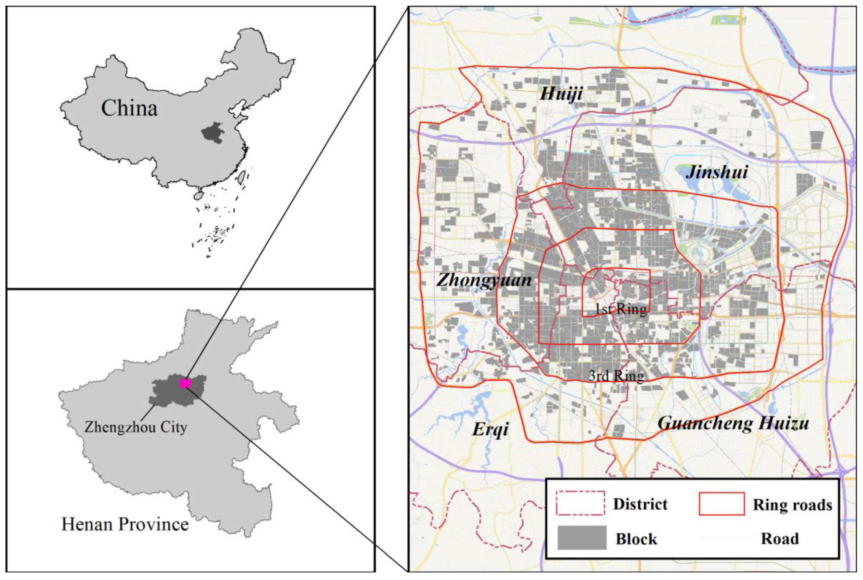
2.1. Study Area

Zhengzhou is located in the central part of China and is an important comprehensive transportation hub of the country. Zhengzhou has witnessed the rapid urbanization progress of China since the economic transformation in 1992. The permanent residential population in urban areas of Zhengzhou increased from 1.84 million to 7.14 million from 1995 to 2017. However, the registered population only increased from 1.36 million to 3.54 million, indicating that more than 3 million non-residents were beyond the welfare of residents. These non-residents are mainly migrants or “rural migrant workers in cities” who often live in villages in cities or urban fringes [31]. Furthermore, employees of state-owned enterprises decreased from 744,300 in 1995 to 432,700 in 2003 and have now stabilized at about 450,000. Zhengzhou’s administrative division includes six districts. Community is the basic unit and place of human life, as well as the basic unit and key link of national governance. Therefore, in this study, according to the land use status data and building data in the Zhengzhou Metropolitan Area Master Plan (2012~2030), the buildings in the residential land type are extracted, and then the residential areas are further identified according to the residential area POI data, and the data of non-residential area types are eliminated. We have identified 2494 residential areas within the Fourth Ring Road of Zhengzhou (Figure 1). Among them, the first ring has 116 blocks, mainly in the old city; the second ring has 699 blocks, mainly old industrial bases and commerce; and the third and fourth rings have 1027 and 652 blocks, respectively, mainly urban villages and urban expansion.

2.2. Data

2.2.1. Social Sensing Data

Based on the Baidu Map development platform, we used Python to mine POI data within the fourth ring of Zhengzhou City (https://lbsyun.baidu.com/ (accessed on 27 September 2018)). Then, according to the Urban Land Classification and Planning Construction Land Standard (http://www.mohurd.gov.cn/wjfb/201201/t20120104_208247.html (accessed on 16 November 2018)), which has been implemented since 2012, the POIs dataset was divided into eight categories, namely residential land, land for public administration and public services, land for commercial service facilities, industrial land, land for logistics and warehousing, land for roads and transportation facilities, land for public utilities, and land for green areas and squares. In order to calculate the infrastructure categories around the residential area, a 600 m buffer zone was made with the residential area as the center, and the number of types of POIs in the buffer zone was calculated, considering the decay law of distance [32].

Rental data from online individual rental records within the fourth ring of Zhengzhou City were released by the Anjuke online real estate platform (https://zhengzhou.anjuke.com/ (accessed on 16 November 2018)). The rental data were mainly obtained by using Python programming language. The main contents include rental price, housing area, housing location, and latitude and longitude. However, the rent data collected did not cover the entire study area, and there was a missing rent component. In order to predict the missing rent values more accurately, the Weka machine learning platform was used for the prediction of missing rent data, and we added normalized difference vegetation index (NDVI), average light brightness values from nighttime light remote sensing data, and infrastructure kernel density (transportation service facilities, education, commerce, etc.) from POI data in the prediction process.

The accessibility data of public service facilities were mainly calculated by using the real-time batch route planning Web API of the Baidu Map development platform (https://lbsyun.baidu.com/ (accessed on 17 October 2020)). The distance and walking time between the residential area and the location of the public service facility were measured. The location of public service facilities is derived from the POI data of the Baidu Map. Regarding the acquisition of data for the Baidu Map development platform, it includes POI data and route planning data for the accessibility of public service facilities. Baidu Maps is similar to Google Maps, which requires us to apply to Baidu Maps to register as a Baidu developer and then create a browser-side application. The Baidu Maps development platform is able to obtain a unique service secret key AK and then use Python programming to obtain it according to the type needed.

2.2.2. Remote Sensing Data

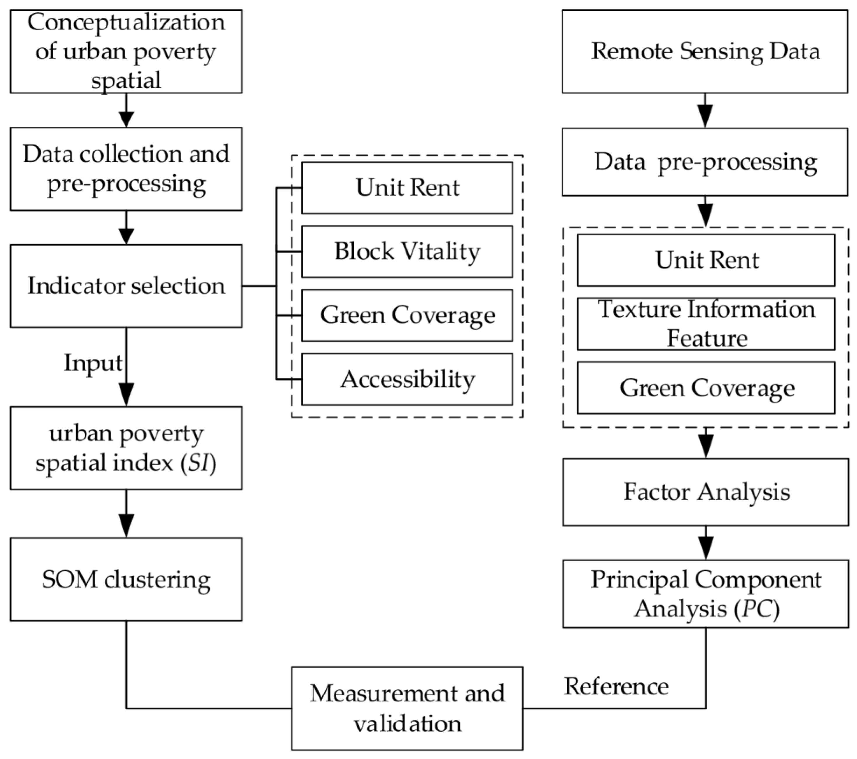
Remote sensing image data at Sentry 2# (https://earthexplorer.usgs.gov/ (accessed on 17 October 2018)) were applied. They were acquired in 2018. The maximum likelihood method was used for supervised classification to extract green space and water bodies. On this basis, high-resolution Google satellite images were used for artificial vectorization complementary recognition, and then the residential area scale green space and water area extraction.

The average lighting intensity value was calculated by Luojia 1# night light remote sensing data (http://59.175.109.173:8888/app/login.html (accessed on 17 October 2018)). The night light remote sensing data of Luojia 1# were acquired in 2018, with a spatial resolution of 130 m. We extracted the average nighttime lighting brightness values for each residential area in ArcGIS.

3. Methods

In the spatial measurement process framework of urban poverty in Figure 2, there are two main steps. First, we give a concept of urban poverty space, construct a model of urban poverty space index based on the selection of corresponding indicators, and then perform SOM clustering on the model results. Moreover, we also performed a comparative validation using the texture feature information from remote sensing data.

3.1. Construction of Measurement Indicators

The spatial measurement of urban poverty consists of four indicators, which are based on previous research [10,26,29,33,34,35]. It is mainly measured from the economic status, built environment, accessibility of public service facilities and vitality of each block, including unit rent, block vitality, green coverage, and accessibility.

3.1.1. Unit Rent

The rent price is a direct reflection of the land green coverage index, the accessibility of public service facilities, and the intensity of community activities, and reflects the economic status of the residents. In metropolitan areas with free housing, urban low-income people are sensitive to housing prices or rent, which is an important measure of urban poverty. In addition, places with high housing prices or rents tend to have high access to subways, parks, and infrastructure. In China, the cost of housing also accounts for a large part of household consumption expenditure. In particular, it has a significant impact on low-income people [26]. Moreover, Leandro-Reguillo and Stuart’s research shows that housing proximity to employment opportunities, education, and health care facilities is positively associated with increased household income [36]. At the same time, rental information can also reflect density, accessibility, and livability to a certain extent [37]. Therefore, the unit rent is calculated as:

R_j = R_totalj/A_j

(1)

where R_j is the unit rent of block j (CNY/m²), R_totalj is the rent of block j (CNY/m²), and A is the housing area of block j (m²).

3.1.2. Block Vitality

Urban vitality reflects the basic elements of human activities and urban life quality in different space–time, such as acceptable urban appearance, developed urban functions, and adequate urban activities [38,39]. Urban vitality is an important evaluation index of urban decline [40]. Therefore, it is used to reflect the diversity of surrounding residential areas or the degree of completion of infrastructure and land use intensity. Density, accessibility, livability, and diversity are important indicators for measuring block-scale activities [29,40]. Therefore, the degree of block vitality is expressed using a diversity index, which is also known as an entropy model of land use mixture. The calculation formula is:

$$V_j =\frac{-{{\displaystyle \sum }}_i\left(M_{ij}ln\left(M_{ij}\right)\right)}{ln{N}_j}$$

(2)

where V_j is the block vitality of block j. M_ij is the proportion of POI of type i in block j. N_j is the number of POI types in block j. V_j values are within [0, 1]. V_j is 0 when there is only one type of POI in the region and it is 1 when the proportions of different POI types in the region are equal.

3.1.3. Green Coverage

Urban green space and urban landscape have an important impact on social sustainability, supporting physical, psychological, and social health, increasing urban comfort, and providing a whole set of ecosystem services to cities [35,41,42]. The green coverage rate of the residential area reflects the quality of the community’s ecological environment. Under different socio-economic and cultural backgrounds, there are few green spaces and low-quality green spaces in urban poverty space [43,44]. Similarly, the construction of green landscapes, green space, and other infrastructure will not only affect the recovery of poverty spaces, but also help residents cope with poverty [45,46]. Therefore, the green coverage index is:

$$L_j=\frac{w_j+G_j}{Z_j}$$

(3)

where L_j is the green coverage index of block j and L ranges within [0, 1]. W_j refers to the water area of block j. G_j is the green land area of block j. Z_j is the total area of block j.

3.1.4. Accessibility

Urban public service facilities are the basic public spaces for community residents to live. The availability of urban public service facilities is one of the important factors affecting residents’ quality of life. Accessibility of public service facilities affects the convenience of residents’ daily life and is also an important symbol reflecting the quality of life of urban residents [47]. According to evidence published by the World Bank, the main difference between those who have escaped chronic poverty and those who remain trapped in poverty is not income, but access to basic services [34]. Accessibility is a standard to measure social equity [48], and an important factor to improve social sustainability [49]. At the socio-economic level, the supply and accessibility of public service facilities affect social equity and justice [50], and it is generally believed that the rich have more accessibility than the poor [51]. Therefore, the accessibility of public service facilities refers to the shortest distance and convenience of residents from the community to public service facilities, and the value of obtaining the most resources and services from public service facilities at the lowest cost. The longer the time spent on accessibility, the worse the resources available for public service facilities. With real-time Internet map-based service API using Python code, the average accessibility to public service facilities of primary schools, middle schools, and large shopping malls by walking is calculated as follows:

$$A=\frac{E_i+M_i+S_i}{n}$$

(4)

where A represents the average accessibility of public service facilities to primary schools, middle schools, and shopping malls by walking. $E_i$ is the time to reach the i primary school. $M_i$ is the time to reach the i middle school. $S_i$ is the time to reach the i large shopping center, and n is the type of public service facilities.

3.2. Modeling Urban Poverty Spaces

In order to measure the urban poverty space, taking into account the factors of the socio-economic and built environment, this paper adopts four indicators: green coverage index, block vitality, unit rent, and average accessibility of public service facilities based on multi-source big data. These four indicators reflect the environmental conditions, built environment, livability, vitality, and convenience of block, and the four indicators are normalized. In the normalization process, the land green coverage index, block vitality, and unit rent are normalized as positive indicators, the calculation formula is:

$$Y_{nm}=X_{nm}-mi{n}_{nm}/ma{x}_{nm}-mi{n}_{nm}$$

(5)

The average accessibility index of public service facilities is reverse normalized, and the calculation formula is:

$$Y_{nm}=ma{x}_{nm}-X_{nm}/ma{x}_{nm}-mi{n}_{nm}$$

(6)

where $X_{nm}$ is the value of n indicator m block, $mi{n}_{nm}$ is the minimum value of n indicator m block, and $ma{x}_{nm}$ is the maximum value of n indicator m block.

This paper uses the multiplier index to construct the urban poverty spatial index according to the selected indicators. Most of the relevant studies use the addend principle, which may define urban poverty measures, but the added principle conveys the idea that the different dimensions are strictly interchangeable with each other [52]. However, the multiplier index emphasizes the importance of the simultaneous existence of all its indicators and emphasizes that all components are essential. The multiplier index is usually written as the geometry of several exponents, the indicators are irreplaceable, and the multiplicative characteristics of this index also follow the construction of the Human Development Index [53]; for example, Brelsford et al. used the census data to determine the four different dimensions of slum dwellers’ access to improved water, improved sanitation, electricity, and permanent housing, and constructed a sustainable development index (X) with a multiplier index [52]. Therefore, the multiplier index is used to construct the urban poverty spatial index (SI):

$$SI=\sqrt[4]{L\times V\times R\times A}$$

(7)

where SI is the urban poverty spatial index of the research unit; the lower the urban poverty spatial index, the higher the urban poverty spatial degree. L is the green coverage index of the research unit. V is the block vitality intensity of the research unit. R is the unit rent of the research unit. A is the average accessibility of public service facilities.

3.3. Self-Organizing Map (SOM) Clustering

Self-Organizing Map network is an unsupervised learning clustering algorithm based on a neural network. Different from the general neural network training based on the backward transfer of the loss function, it uses a competitive learning strategy, relying on the competition between neurons to gradually optimize the network. It uses the nearest neighbor function to maintain the topology of the input space. The self-organizing map network is also a single-layer neural network, including an input layer and a competition layer. The competition layer has a topological structure composed of a series of nodes composed of neurons, which can be a one-dimensional structure or a two-dimensional structure. The minimum number of nodes in the competition layer is $5\sqrt{N}$ (N: the number of training samples). SOM plays the role of dimensionality reduction and can map high-dimensional input data into one-dimensional or two-dimensional space. The hidden node of a one-dimensional topological relationship is a line, and the hidden point of a two-dimensional topological relationship is a plane. After the topological relationship is determined, the calculation process starts, which is mainly divided into [54]:

(1)

Initialize the SOM. Each node randomly initializes its parameters. The number of parameters for each node is the same as the dimension of the input.

(2)

Finding the Best Matching Unit (BMU). Iterate through each node in the competing layer and calculate the similarity between them, and select the node with the smallest distance as the (BMU). The similarity is usually defaulted to Euclidean distance, which can be calculated below:

$$d\left(x,y\right)=\sqrt{{\displaystyle \sum }_{i=1}^n{\left(x_i-y_i\right)}^2}$$

(8)

(3)

Learning Rate. The learning rate of the SOM decays as the number of iterations increases.

$$\alpha \left(t\right)={\alpha }_0\times {\left(\frac{{\alpha }_{end}}{{\alpha }_0}\right)}^{\raisebox{1ex}{$t$}\!\left/ \!\raisebox{-1ex}{$t_{max}$}\right.}$$

(9)

where $\alpha \left(t\right)$ is the learning rate, $t$ is the number of iterations, ${\alpha }_0$ is the start value, ${\alpha }_{end}$ is the end value, and $t_{max}$ is the maximum number of iterations.

(4)

Neighborhood Function. The neighborhood function is used to determine the influence of the best matching unit on its nearest neighbor nodes.

$$\sigma \left(t\right)={\sigma }_0\times \left(1-\frac{t}{t_{max}}\right)$$

(10)

where $\sigma \left(t\right)$ represents neighborhood, and ${\sigma }_0$ is the starting value of the neighborhood function.

(5)

Neighborhood Distance Weight. The neighborhood distance weights indicate the number of iterations and the distance between BMU and other nodes. The distance between BMU and nodes is Euclidean distance by default. Therefore, the neighborhood distance weights are defined as:

$$h_{i,j}\left(t\right)=\exp \left(-\frac{d^2}{2\times \sigma {\left(t\right)}^2}\right)$$

(11)

where $h_{i,j}$ represents the neighborhood distance weight between BMU and node.

(6)

Adapting Weights. The weights of the SOM are adjusted according to the learning rate and the neighborhood distance weights.

$$w_i\left(t+1\right)=w_i\left(t\right)+\alpha \left(t\right)\times h_{i,j}\left(t\right)\times \left(x\left(t\right)-w_i\left(t\right)\right)$$

(12)

where $h_{i,j}\left(t\right)$ represents the neighborhood function, $\alpha \left(t\right)$ is the learning rate, x(t) is the present data point, and $w_i\left(t\right)$ is the weight vector of node i at iteration t.

3.4. SI Validation

Structural and textural features of remote sensing data for the study of urban inner-city poverty have been applied. Duque et al. used the structure and texture feature values of remote sensing data images and principal component analysis to identify inner-city poverty in Medellin, Colombia [19]. Yuan et al. extracted texture eigenvalues from remote sensing data, land cover types, and unit rent indicators to measure inner-urban poverty in Guangzhou, China, by principal component analysis [55]. Therefore, in this paper, first, we use the gray level co-occurrence matrix (GLCM) to extract the mean, variance, homogeneity, contrast, dissimilarity, entropy, angular second moment, and correlation indicators of texture information feature statistics in remote sensing images, as well as land green coverage degree and unit rent. Moreover, we use the factor analysis of the principal component analysis method to perform KMO (Kaiser–Meyer–Olkin) and Bartlett sphericity tests on the standardized indicators, and further compare the KMO values of each band. Finally, the principal components corresponding to the eigenvalues with higher cumulative contribution rates are selected. Therefore, the measurement space of urban poverty based on the principal component analysis method is:

$$PC={\displaystyle \sum }_{j=1}^n({\alpha }_j\times {\alpha }_{ij})$$

(13)

where ${\alpha }_{ij}$ is the score of residential area $i$ in indicator $j$, and ${\alpha }_j$ is the variance contribution rate of indicator $j$. The lower the score, the higher the spatial degree of urban poverty.

4. Results

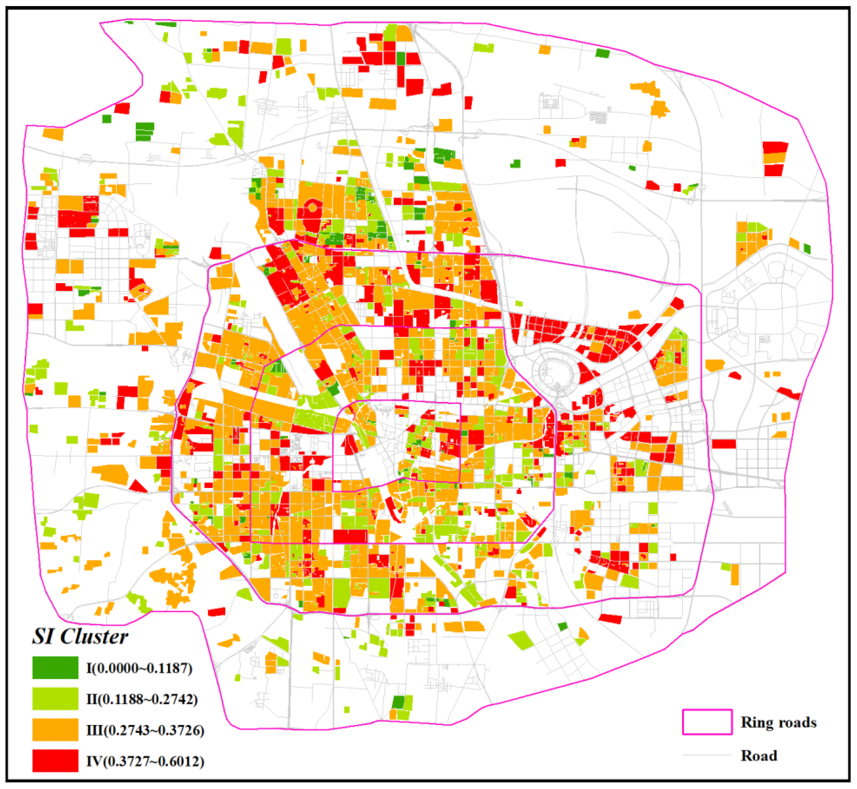
4.1. Structural Features of Urban Poverty Spaces

The structural characteristics of urban poverty space are mainly caused by the spatial differentiation of factors such as green coverage index, block vitality, unit rent, and average accessibility of urban public services.

The spatial distribution of unit rents shows a roughly high pattern on the outside and low pattern in the inner city (Figure 3a). Due to the continuous expansion of the city, most of the houses between the second and third ring lines of the city are new residential areas built in recent years. The housing conditions and surrounding environment are relatively sufficient, especially the construction of the eastern new district of Zhengzhou City; additionally, the ecological environment is adequate, and the built environment is superior, with high-quality public service facilities. Part of the area between the Third Ring Road and the Fourth Ring Road is still under development and construction, so the rents of units in areas with complete facilities are higher. The areas with lower unit rents in these areas are far from public service facilities, and the basic service facilities are relatively weak. In the inner city center area of the First Ring Road, the housing is old, the surrounding environment is aging, and the unit rent price is low.

The overall block vitality is irregularly distributed (Figure 3b), and each area has areas with high block vitality, which is mainly related to the service radius of urban infrastructure and urban planning. The area with low block vitality is in the southeastern part of Guancheng Hui District, that is, the southern part of the part between the Second Ring Road and the Third Ring Road. The main reason is that there are concentrated industrial areas in this area, and the layout of infrastructure and public service facilities is relatively simple. The areas with the highest block vitality are concentrated in the southwest area of the Fourth Ring Road, mainly because these areas are close to universities, industrial areas, and residential areas outside the Fourth Ring Road and have a high degree of land use mix.

The green coverage index is higher in the outer urban areas than in the central urban areas, with the highest green coverage in the new eastern urban areas (Figure 3c). This area is guided by the ecological city, symbiotic city, and metabolic city planning concepts, and has a better ecological environment. The outer areas of the city are dominated by the land to be developed and the land under development, the green environment is poor, and the green coverage index is lower than that of the new urban area. Moreover, in the commercial core area of the old urban area, the land price is high and the building density is tight, so the green coverage index is low.

The spatial distribution pattern of the average accessibility of public service facilities shows that the accessibility of residential areas in the city center is higher than that of residential areas outside the city (Figure 3d). This is mainly because the urban center residential area has been built for a long time, the basic service facilities are more developed, the population mobility and density in the urban center are high, and large commercial centers are also concentrated there, so the accessibility of public service facilities is high. With the continuous increase in the population of Zhengzhou City, the expansion and planning of the city, and the continuous improvement of basic service facilities from the central area of the city to the periphery, the distance between residential areas and basic service facilities has reduced. The area near the Fourth Ring Road on the periphery of the city is the area where the city is expanding and renovating. The population density is small and the infrastructure services are weak. Therefore, the farther the residential areas outside the city are from the basic service facilities, the poorer the accessibility.

4.2. Classification Features of Urban Poverty Space

According to the model measurement of urban poverty space, the classification of urban poverty space adopts a self-organizing mapping neural network structure with a competition layer of 2 × 2, where the number of iterations is 1000, the initial learning rate is 1, and the number of steps in the sorting stage is 2000. The space is divided into four clusters (Figure 4).

The Class I living environment is the worst, with few numbers, scattered in space and with an independent distribution. They are mainly distributed in the northern part of Jinshui District and the southern part of Huiji District, and are scattered and less prevalent in other areas. Among them, within the first ring line, the second ring line, the third ring line, and the fourth ring line account for 10.26%, 5.95%, 6.80%, and 20.63% of each ring line block, respectively. The Fourth Ring Road area accounts for a large proportion of the residential area. This is mainly because there are large-scale urban villages in the north of Jinshui District and the south of Huiji District. This category is a key area for improving the quality of the built environment and urban renewal.

The Class II living environment is relatively poor, mainly in old urban areas and residential areas with long-standing buildings. Cities in these regions have low rent prices, aging infrastructure, and high population densities. Another part of the area is mainly the old industrial area and the unit residential area under the planned economy system. This part of the area has low rent prices and a long construction time. Retired workers in the old industrial area still have a strong attachment to this area and still retain their traditional way of life. Therefore, the block vitality in these areas is relatively high. As Jane Jacobs believes, land use intensity, density, block size, and building age are the conditions that must be met to maintain urban vitality [56].

The Class III living environment is better. This type of residential area is sparsely distributed in the first ring of the city, and more distributed between the second ring and the third ring. This part of the area accounts for a large proportion of the fourth ring residential area. With the urbanization and real estate market economy, the expansion of cities, the upgrading of residential area planning, and the continuous improvement of public service facilities, inner city residents and some middle-class residents with strong economic foundations will choose to live in these areas with better conditions.

The Class IV living environment is the best. The spatial distribution presents a spatial pattern in which the eastern New District of Zhengzhou is relatively continuous and other areas are relatively scattered. Mainly in new urban areas, these areas are mainly modern new urban areas planned by the government according to high standards and high starting points. This part of the area has a superior living environment, higher unit rents, a better built environment, sound public service facilities, and many universities and companies.

5. Discussions

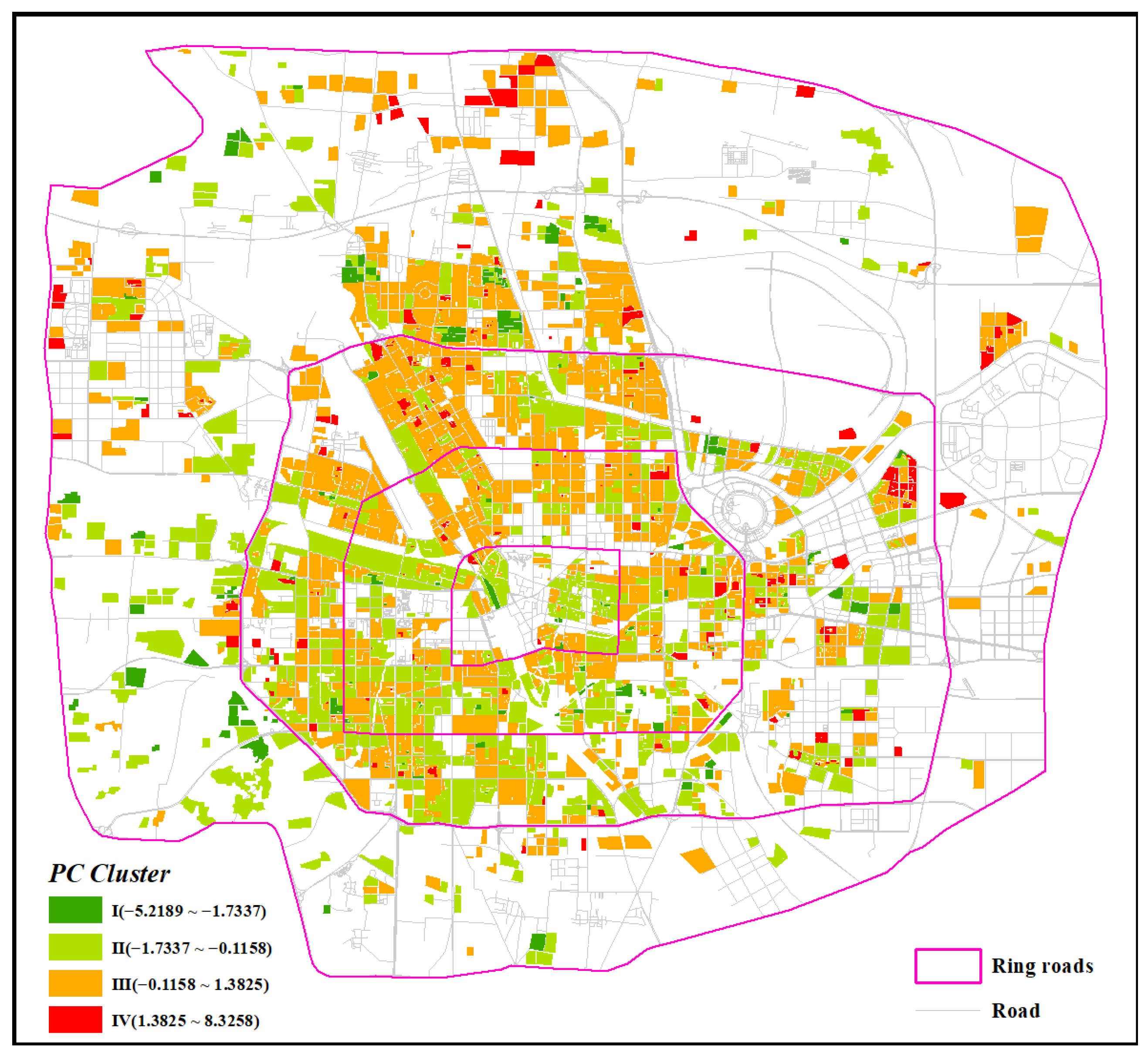
5.1. Model Comparison and Validation

Based on the spatial measurement of poverty in urban inner cities by the principal component analysis method, we selected the third band with a large KMO value. The KMO value of the third band is 0.787, the degree of freedom is 45, and the significance is 0.000. The KMO (Kaiser–Meyer–Olkin) and Bartlett’s sphericity test are better, and the factor analysis of principal component analysis can be further executed. Finally, the principal components corresponding to the eigenvalues with a cumulative contribution rate of 83.862% were selected (

Table 1. Principal component analysis method total variance interpretation.

Component	Eigenvalue			Loading Sum of Squares
	Total	Variance (%)	Accumulative %	Total	Variance (%)	Accumulative %
1	6.121	61.211	61.211	6.121	61.211	61.211
2	1.262	12.624	73.835	1.262	12.624	73.835
3	1.003	10.027	83.862	1.003	10.027	83.862
4	0.784	7.835	91.697
5	0.521	5.206	96.903
6	0.229	2.289	99.192
7	0.052	0.519	99.711
8	0.023	0.229	99.94
9	0.005	0.051	99.991
10	0.001	0.009	100

). The eigenvalues of each principal component were greater than 1, and then the total score of the three extracted principal components was calculated.

It can be seen from the spatial distribution of the urban poverty spatial results measured based on principal component analysis (Figure 5) that the spatial distribution of the low-value area (Class I) of the urban poverty spatial is mainly in the area between the Third Ring Road and the Fourth Ring Road. This is followed by a sparse distribution within the first and second rings, and these Class I areas account for 7.8% of all residential areas within the fourth ring of Zhengzhou. The area between the Third Ring Road and the Fourth Ring Road belongs to the fringe of the built-up area of the city and is dominated by urban villages and bare plots of land, most of which are under construction or undeveloped after the demolition of urban villages. Within the First and Second Ring Roads, there are also fewer Class I residential areas. In these areas, the use of texture features of remote sensing data to measure urban poor spaces or areas with poorly built environments is often affected by the physical surface of residential areas and the appearance of buildings, which may affect the performance of measurement and recognition.

In the comparison of the two models, we extracted the spatial distribution of the first type of urban poverty space measured by the spatial index of urban poverty and based on the method of principal component analysis. As can be seen in Figure 6, most of the urban poor spaces commonly identified by both are located in the area between the Third and Fourth Ring Roads. The common urban poor spaces identified by both are mainly former urban village areas, which after demolition have now become undeveloped or developing bare land settlements. Moreover, the difference between the two measures of effectiveness is mainly in the old urban areas of the inner city and the bare land on the fringes of the built-up urban areas. In old urban areas, SI can measure the residential areas with poor-quality living environments in the old urban areas. However, the principal component analysis method based on remote sensing data is influenced by the appearance of buildings, which may affect the accuracy of identification. Bare land on the fringe of built-up urban areas is influenced by human activities and urban vitality buffer zones. The accuracy of the measurement by the principal component analysis method based on remote sensing data is higher than that measured by SI.

To validate the identified typical urban poverty spaces, the Class I poverty spaces measured by SI and PC are mainly divided into four types (Figure 6). Moreover, to further validate the four typical urban poverty spaces, we visualized the land use changes in the four typical urban poverty spaces using VHR remote sensing satellite images (Figure 7). Figure 7a shows the old urban areas of the city, which are old and have poor built environment quality. Figure 7b shows the urban villages close to the built-up areas, which have been demolished with the development of urbanization. Figure 7c indicates the urban villages that are far from the built-up area. Figure 7d indicates exposed or unused residential areas, urban villages before demolition at the edge of built-up areas, and exposed residential areas after demolition.

Moreover, the data and methods used by SI and PC in measuring the urban poverty space are different. The measurement of the principal component analysis method based on remote sensing data shows that the texture features of remote sensing data can be affected by the physical surface of the settlement and the structure of the building exterior, which may affect the measurement and identification. Exposed land on the edge of built-up urban areas can be better identified. However, the urban poverty space measured based on the urban poverty spatial index indicates that there is a better measurement and identification effect in residential areas with poorly built environments in old urban areas, urban villages, and bare residential areas in urban villages after demolition. In addition, the measurement of urban poverty space based on remote sensing data takes more into account the physical form and often ignores the socio-economic and built environment factors. However, the use of social sensing data can better fill the gap in measuring urban poverty space with remote sensing data.

5.2. The Role of SI Methods in Mapping Urban Poverty Spatial

Sustainable cities and communities are among the goals of the United Nations for sustainable development and are essential to humanity’s pursuit of sustainable urban development. Urban poverty spaces have different connotations in each country and region. In this paper, more consideration is given to the built environment, housing affordability, living environment, and access to basic services and facilities, the improvement of which can better improve the quality of life and happiness of the people. In particular, the vulnerability of many cities is caused by the lack of adequate and affordable housing, public health systems, and inadequate access to basic services at the beginning of the COVID-19 outbreak [57]. Although scholars have used different data and methods to measure urban poverty, the focus of attention varies across countries and regions, and the results of urban poverty measures vary. Therefore, to better fit the local situation, this paper measures urban poverty space at a fine scale using remote sensing data and social sensing data, which are massive, multi-source, heterogeneous, and multi-temporal in nature, and also have strong spatiotemporal and physical correlations.

A healthy built environment benefits community sustainability and promotes healthy lifestyles, especially high-density and mixed-use blocks, accessibility, and a high presence of urban amenities [36]. The four indicators of the spatial model of urban poverty affect and interact with each other, where any component is related to each other, and each indicator is equally important. Meanwhile, green coverage, block vitality, unit rent, and accessibility all have a large impact on urban poverty space. Green vegetation plays an important role in the sustainable development of society, and there is a spatial non-smoothness between the human-perceived green landscape and the urban poverty space [10]. Block vitality is the diversity of urban life; the people, spaces (places), and things in the city are the basis of the diversity of urban life [58]. Housing affordability is critical to meeting the needs of individuals, and for people in different socio-economic groups, access to housing that meets socially acceptable standards will contribute to the sustainability of society [35,59]. The ability to access infrastructure services also has a direct impact on unit rents and block dynamics. Furthermore, the spatial location of public service infrastructure also influences the distribution of urban poverty space.

Moreover, COVID-19 has already had a severe impact on urban poverty, with more than 90% of cases occurring in urban areas, and has also exacerbated the dilemma of the world’s densely populated informal settlements and slum dwellers [60]. Therefore, in the context of global climate change and urbanization, more attention should be paid in the future to the vulnerability of the urban poverty space to climate change, the inequality of social resources, and the inequality of air pollution. To gain access to livelihoods, these informal settlements or slums are often vulnerable to sea level rise, flooding, landslides, and heat waves [61]. Furthermore, the spatial distribution of urban poverty is also a region of the poorer built environment, vulnerable to inequalities in air pollution. For example, the use of air purifiers for the relatively wealthy population keeps them safe from air pollution [62]. Moreover, for regions that are lagging in economic development and information technology, access to open geographic big data and government census data should be enhanced in the future, and smarter, more effective, and more accurate artificial intelligence and deep learning technologies should be used to capture the characteristics of urban poverty and to map urban poverty.

5.3. Strengths and Weaknesses

The biggest contribution of this paper is the use of multi-source big data to integrate the built environment, economic status, and residential environment into an urban poverty spatial index model. More attention has been paid to the built environment, housing affordability, and living environment. At the same time, the use of the multiplicative index emphasizes the mutual influence and interaction between the indicators, and any one component is related to another, and is equally important and cannot be replaced by another. In addition, the use of multi-source big data makes up for the long time, high cost, and lagging data quality of traditional data. At the microscopic scale, it also avoids the “ecological fallacy” of remote sensing data in identifying poverty spaces in the inner city and the influence of the physical surface of the settlement and the structure of the building’s appearance. Therefore, it provides a comprehensive, low-cost, and efficient monitoring method for the refined management of urban poverty space, and also provides theoretical and technical support for the improvement of urban built environment quality, sustainable urban development, urban renewal, and planning.

Furthermore, although the study in this paper has its merits, we must admit that some limitations need to be addressed in future research. Firstly, due to the influence of humanities, social economy, built environment, and gentrification within the city, the spatial measurement of urban poverty in rapidly urbanizing areas is complicated [63]. A small number of communities in the old urban area occupy location advantages and are close to school districts, resulting in higher housing prices and lower green coverage, which may also overestimate or underestimate the identified urban poverty space. Therefore, how to further optimize it needs to be discussed in depth in future research. Secondly, the area studied in this paper is the urban built-up area. However, affected by the phenomenon of urban suburbanization, the infrastructure and public service facilities in these areas are not as complete as those in urban built-up areas, and high-end suburban communities with high green coverage and low accessibility may appear. How to further study the spatial measurement of poverty in the whole city still needs to be explored. Thirdly, due to the COVID-19 epidemic, for its prevention and control, and for safety reasons, this study did not conduct a questionnaire survey on the spatial measurement of urban poverty at the block scale. In the future, big data and traditional survey data should be combined for comparative research. Lastly, this model may be a better fit for rapidly urbanizing and relatively developed informatization places. Other indicators and methods may be needed to measure regions with slow urbanization and information technology development.

6. Conclusions

This paper measures urban poverty using remote sensing data, POI data, Baidu Map API path planning data, and online rent data. Block green space coverage, block vitality, accessibility to public service facilities, and per unit rent have been quantified as the indicators of poverty. From the perspective of the built environment, economic status, and block environment, the multiplier index is used to construct the urban poverty spatial index model. It is more reflected in the quality of the habitat, the level of infrastructure, and the socio-economic dimension of the resident. Taking the main urban area of Zhengzhou as an example, the SOM artificial neural network model is used to classify the urban poverty spatial index. The spatial differentiation pattern of urban poverty in its main urban area was revealed and compared and validated the urban poverty space based on remote sensing data measurement. The main findings of this study can be summarized as follows.

Firstly, this paper uses the multiplier index to construct the urban poverty spatial index through the coverage of block green space, the vitality of the block, the accessibility of public service facilities, and the unit rent. The importance of the simultaneous existence of all its indicators is emphasized. The four indicators of the spatial model of urban poverty affect and interact with each other, and any one component is related to another. Taking the built environment, economics, and living environment into consideration is conducive to the sustainable development of the community and the promotion of healthy lifestyles, especially high-density and mixed-use blocks, accessibility, and areas with a high presence of urban amenities. Therefore, the study can provide a comprehensive, low-cost, efficient, and dynamic monitoring method for the fine management of urban poverty space, and also provide theoretical support and technical support for the improvement of urban built environment quality, sustainable development of cities, urban renewal, and planning.

Secondly, based on the SOM artificial neural network model clustering, the urban poverty spatial index models are divided into four categories. Class I urban poverty space is a key area of concern for improving the quality of the built environment and urban renewal. Four typical types were identified based on Class I urban poverty spaces, namely old urban areas in inner cities, urban villages, urban villages after demolition, and bare land.

Moreover, in model comparison and accuracy validation, the texture features of remote sensing data are affected by the physical surface of the settlement and the structure of the building exterior, which may impact the effectiveness of the measurement and recognition. The remote sensing data have an adequate recognition effect on the bare land at the edge of the built-up area of the city. However, the urban poverty space measured based on the urban poverty spatial index indicates that there is a better measurement and identification effect in residential areas with a poor built environment in old urban areas, urban villages, and bare residential areas in urban villages after demolition. In addition, the measurement of urban poverty space based on remote sensing data takes more into account the physical form of the ground surface and often ignores the socio-economic and built environment factors. However, the use of multi-source big data can better compensate for the lack of remote sensing data to measure urban poverty space. In addition, these multi-source big data can also make up for the time-consuming, costly, and data lag characteristics of traditional data. At the microscopic scale, it also avoids the “ecological fallacy” of remote sensing data in identifying poor spaces in the inner city and the influence of the physical surface of the settlement and the structure of the building’s appearance.

In addition, this paper provides some policy implications. For the improvement of the quality of the built environment, the government needs to plan, repair, rebuild, and improve areas with poor quality building structures, dilapidated residential areas in the city, urban villages, and poor living conditions, thus improving the quality of the built environment and urban landscape in residential areas. In the community, the degree of public participation should be actively promoted to facilitate the restoration and renewal of dilapidated buildings from the bottom up. The concept of community life circle should be used to improve the service scope of spatial resources of public service facilities, increase the flexibility and resilience of the process of using public service facilities, reasonably plan the demand and supply between public service facilities, and continuously promote the development of accessibility and equalization from communities to public service facilities.

Finally, in the context of global climate change and urbanization, more attention should be paid in the future to the vulnerability of poverty areas to climate change adaptation and the inequality of air pollution. Moreover, for regions lagging in economic development and information technology, access to open geographic big data and government census data should be enhanced in the future, and smarter, more effective, and accurate artificial intelligence and deep learning technologies should be used to capture the characteristics of urban poverty and map urban poverty in a more refined and dynamic way.

References

1. Wratten, E. Conceptualizing urban poverty. Environ. Urban. 1995, 7, 11–36. [Google Scholar] [CrossRef]
2. Klopp, J.M.; Petretta, D.L. The urban sustainable development goal: Indicators, complexity and the politics of measuring cities. Cities 2017, 63, 92–97. [Google Scholar] [CrossRef]
3. Lucci, P.; Bhatkal, T.; Khan, A. Are we underestimating urban poverty? World Dev. 2018, 103, 297–310. [Google Scholar] [CrossRef]
4. UN-Habitat. UN Human Settlements Programme, Global Urban Indicators Database, Nairobi, Info on Population in Slums (% of Urban Population); United Nations Human Settlement Programme: Nairobi, Kenya, 2016.
5. Des, U. World Economic and Social Survey 2013: Sustainable Development Challenges; United Nations, Department of Economic Social Affairs: New York, NY, USA, 2013; pp. 123–136.
6. Un, D. Revision of the World Urbanization Prospects; United Nations Department of Economics and Social Affairs, Population Division: New York, NY, USA, 2014.
7. Padda, I.U.; Hameed, A. Estimating multidimensional poverty levels in rural Pakistan: A contribution to sustainable development policies. J. Clean. Prod. 2018, 197, 435–442. [Google Scholar] [CrossRef]
8. Neamtu, B. Measuring the Social Sustainability of Urban Communities: The Role of Local Authorities. Transylv. Rev. Adm. Sci. 2012, 8, 112–127. [Google Scholar]
9. Li, X.; Kleinhans, R.; van Ham, M. Shantytown redevelopment projects: State-led redevelopment of declining neighbourhoods under market transition in Shenyang, China. Cities 2018, 73, 106–116. [Google Scholar] [CrossRef] [Green Version]
10. Meng, Y.; Xing, H.F.; Yuan, Y.; Wong, M.S.; Fan, K.X. Sensing urban poverty: From the perspective of human perception-based greenery and open-space landscapes. Comput. Environ. Urban 2020, 84, 101544. [Google Scholar] [CrossRef]
11. Noble, M.; Wright, G.; Smith, G.; Dibben, C. Measuring multiple deprivation at the small-area level. Environ. Plann. A 2006, 38, 169–185. [Google Scholar] [CrossRef]
12. Undp. Human Development Report 1997; Oxford University: Oxford, UK, 1997.
13. Alkire, S.; Santos, M.E. Acute Multidimensional Poverty: A New Index for Developing Countries; University of Oxford: Oxford, UK, 2010. [Google Scholar]
14. Langlois, A.; Kitchen, P. Identifying and measuring dimensions of urban deprivation in Montreal: An analysis of the 1996 census data. Urban Stud. 2001, 38, 119–139. [Google Scholar] [CrossRef]
15. Mitlin, D.; Satterthwaite, D. Urban Poverty in the Global South: Scale and Nature, 1st ed.; Routledge: London, UK, 2012. [Google Scholar]
16. Sabry, S. How poverty is underestimated in Greater Cairo, Egypt. Environ. Urban. 2010, 22, 523–541. [Google Scholar] [CrossRef] [Green Version]
17. Hofmann, P. Detecting Informal Settlements from IKONOS Image Data Using Methods of Object Oriented Image Analysis-an Example from Cape Town (South Africa). In Proceedings of the Remote Sensing of Urban Areas/Regensburger Geographische Schriften, Regensburg, Germany, 12–14 September 2001; pp. 107–118. [Google Scholar]
18. Niebergall, S.; Loew, A.; Mauser, W. Integrative assessment of informal settlements using VHR remote sensing data—The Delhi case study. IEEE J. Sel. Top. Appl. Earth Obs. Remote Sens. 2008, 1, 193–205. [Google Scholar] [CrossRef]
19. Duque, J.C.; Patino, J.E.; Ruiz, L.A.; Pardo-Pascual, J.E. Measuring intra-urban poverty using land cover and texture metrics derived from remote sensing data. Landsc. Urban Plan. 2015, 135, 11–21. [Google Scholar] [CrossRef]
20. Kit, O.; Ludeke, M.; Reckien, D. Texture-based identification of urban slums in Hyderabad, India using remote sensing data. Appl. Geogr. 2012, 32, 660–667. [Google Scholar] [CrossRef]
21. Elvidge, C.D.; Sutton, P.C.; Ghosh, T.; Tuttle, B.T.; Baugh, K.E.; Bhaduri, B.; Bright, E. A global poverty map derived from satellite data. Comput. Geosci. 2009, 35, 1652–1660. [Google Scholar] [CrossRef]
22. Li, G.E.; Cai, Z.L.; Liu, X.J.; Liu, J.; Su, S.L. A comparison of machine learning approaches for identifying high-poverty counties: Robust features of DMSP/OLS night-time light imagery. Int. J. Remote Sens. 2019, 40, 5716–5736. [Google Scholar] [CrossRef]
23. Keola, S.; Andersson, M.; Hall, O. Monitoring Economic Development from Space: Using Nighttime Light and Land Cover Data to Measure Economic Growth. World Dev. 2015, 66, 322–334. [Google Scholar] [CrossRef]
24. Ebener, S.; Murray, C.; Tandon, A.; Elvidge, C.C. From wealth to health: Modelling the distribution of income per capita at the sub-national level using night-time light imagery. Int. J. Health Geogr. 2005, 4, 5. [Google Scholar] [CrossRef] [Green Version]
25. Stark, T.; Wurm, M.; Zhu, X.X.; Taubenbock, H. Satellite-Based Mapping of Urban Poverty With Transfer-Learned Slum Morphologies. IEEE J.-Stars 2020, 13, 5251–5263. [Google Scholar] [CrossRef]
26. Niu, T.; Chen, Y.M.; Yuan, Y. Measuring urban poverty using multi -source data and a random forest algorithm: A case study in Guangzhou. Sustain. Cities Soc. 2020, 54, 102014. [Google Scholar] [CrossRef]
27. Ibrahim, M.R.; Haworth, J.; Cheng, T. URBAN-i: From urban scenes to mapping slums, transport modes, and pedestrians in cities using deep learning and computer vision. Environ. Plan B-Urban 2021, 48, 76–93. [Google Scholar] [CrossRef] [Green Version]
28. Blumenstock, J.; Cadamuro, G.; On, R. Predicting poverty and wealth from mobile phone metadata. Science 2015, 350, 1073–1076. [Google Scholar] [CrossRef] [PubMed]
29. Ta, N.; Kwan, M.P.; Lin, S.T.; Zhu, Q.Y. The activity space-based segregation of migrants in suburban Shanghai. Appl. Geogr. 2021, 133, 102499. [Google Scholar] [CrossRef]
30. Goel, E.; Abhilasha, E.; Goel, E.; Abhilasha, E. Random forest: A review. Int. J. Adv. Res. Comput. Sci. Softw. Eng. 2017, 7, 251–257. [Google Scholar] [CrossRef]
31. Wong, D.F.K.; Li, C.Y.; Song, H.X. Rural migrant workers in urban China: Living a marginalised life. Int. J. Soc. Welf. 2007, 16, 32–40. [Google Scholar] [CrossRef]
32. Su, S.L.; Pi, J.H.; Xie, H.; Cai, Z.L.; Weng, M. Community deprivation, walkability, and public health: Highlighting the social inequalities in land use planning for health promotion. Land Use Policy 2017, 67, 315–326. [Google Scholar] [CrossRef]
33. Chen, Y.M.; Liu, X.P.; Li, X.; Liu, Y.L.; Xu, X.C. Mapping the fine-scale spatial pattern of housing rent in the metropolitan area by using online rental listings and ensemble learning. Appl. Geogr. 2016, 75, 200–212. [Google Scholar] [CrossRef]
34. Benevenuto, R.; Caulfield, B. Measuring access to urban centres in rural Northeast Brazil: A spatial accessibility poverty index. J. Transp. Geogr. 2020, 82, 102553. [Google Scholar] [CrossRef]
35. Yildiz, S.; Kivrak, S.; Gultekin, A.B.; Arslan, G. Built environment design-social sustainability relation in urban renewal. Sustain. Cities Soc. 2020, 60, 102173. [Google Scholar] [CrossRef]
36. Leandro-Reguillo, P.; Stuart, A.L. Healthy Urban Environmental Features for Poverty Resilience: The Case of Detroit, USA. Int. J. Environ. Res. Public Health 2021, 18, 6982. [Google Scholar] [CrossRef]
37. Heyman, A.V.; Sommervoll, D.E. House prices and relative location. Cities 2019, 95, 102373. [Google Scholar] [CrossRef]
38. Jin, X.B.; Long, Y.; Sun, W.; Lu, Y.Y.; Yang, X.H.; Tang, J.X. Process funding Evaluating cities’ vitality and identifying ghost cities in China with emerging geographical data. Cities 2017, 63, 98–109. [Google Scholar] [CrossRef]
39. Delclos-Alio, X.; Miralles-Guasch, C. Looking at Barcelona through Jane Jacobs’s eyes: Mapping the basic conditions for urban vitality in a Mediterranean conurbation. Land Use Policy 2018, 75, 505–517. [Google Scholar] [CrossRef]
40. Zeng, C.; Song, Y.; He, Q.S.; Shen, F.X. Spatially explicit assessment on urban vitality: Case studies in Chicago and Wuhan. Sustain. Cities Soc. 2018, 40, 296–306. [Google Scholar] [CrossRef]
41. La Rosa, D.; Takatori, C.; Shimizu, H.; Privitera, R. A planning framework to evaluate demands and preferences by different social groups for accessibility to urban greenspaces. Sustain. Cities Soc. 2018, 36, 346–362. [Google Scholar] [CrossRef]
42. Jennings, V.; Larson, L.; Yun, J. Advancing Sustainability through Urban Green Space: Cultural Ecosystem Services, Equity, and Social Determinants of Health. Int. J. Environ. Res. Public Health 2016, 13, 196. [Google Scholar] [CrossRef] [Green Version]
43. Brown, C.; Bramley, G.; Watkins, D. Urban Green Nation: Building the Evidence Base; Heriot-Watt University: Dubai, United Arab Emirates, 2010. [Google Scholar]
44. Roe, J.J.; Aspinall, P.A.; Thompson, C.W. Coping with Stress in Deprived Urban Neighborhoods: What Is the Role of Green Space According to Life Stage? Front. Psychol. 2017, 8, 1760. [Google Scholar] [CrossRef] [Green Version]
45. Pares, M.; Blanco, I.; Fernandez, C. Facing the Great Recession in Deprived Urban Areas: How Civic Capacity Contributes to Neighborhood Resilience. City Community 2018, 17, 65–86. [Google Scholar] [CrossRef]
46. Kuo, F.E. Coping with poverty-Impacts of environment and attention in the inner city. Environ. Behav. 2001, 33, 5–34. [Google Scholar] [CrossRef]
47. Zeng, W.; Xiang, L.L.; Zhang, X.L. Research in spatial pattern of accessibility to community service facilities and spatial deprivation of low income communities in Nanjing. Hum. Geogr. 2017, 32, 79–87. [Google Scholar]
48. Doust, K. Toward a typology of sustainability for cities. J. Traffic Transp. Eng. 2014, 1, 180–195. [Google Scholar] [CrossRef] [Green Version]
49. Wong, W.S.; Chan, E.H. Building Hong Kong: Environmental Considerations; Hong Kong University Press: Hong Kong, China, 2000; Volume 1. [Google Scholar]
50. Macintyre, S.; Macdonald, L.; Ellaway, A. Do poorer people have poorer access to local resources and facilities? The distribution of local resources by area deprivation in Glasgow, Scotland. Soc. Sci. Med. 2008, 67, 900–914. [Google Scholar] [CrossRef] [PubMed] [Green Version]
51. Farrington, J.; Farrington, C. Rural accessibility, social inclusion and social justice: Towards conceptualisation. J. Transp. Geogr. 2005, 13, 1–12. [Google Scholar] [CrossRef]
52. Brelsford, C.; Lobo, J.; Hand, J.; Bettencourt, L.M.A. Heterogeneity and scale of sustainable development in cities. Proc. Natl. Acad. Sci. USA 2017, 114, 8963–8968. [Google Scholar] [CrossRef] [PubMed] [Green Version]
53. Herrero, C.; Martinez, R.; Villar, A. Multidimensional Social Evaluation: An Application To the Measurement of Human Development. Rev. Income Wealth 2010, 56, 483–497. [Google Scholar] [CrossRef]
54. Riese, F.M.; Keller, S.; Hinz, S. Supervised and Semi-Supervised Self-Organizing Maps for Regression and Classification Focusing on Hyperspectral Data. Remote Sens. 2020, 12, 7. [Google Scholar] [CrossRef] [Green Version]
55. Yuan, Y.; Liu, J.; Chen, Y.M.; You, Z.Y. Poverty measurement of urban internal space based on remote sensing images and online rental information: A case study of the city core of Guangzhou. Hum. Geogr. 2018, 33, 60–67. [Google Scholar] [CrossRef]
56. Fuller, M.; Moore, R. An Analysis of Jane Jacobs’s: The Death and Life of Great American Cities; Macat Library: London, UK, 2017. [Google Scholar]
57. UN. High-Level Political Forum on Sustainable Development, Convened under the Auspices of the Economic and Social Council; Report of the Secretary-General; United Nations: New York, NY, USA, 2021.
58. Faria, J.R.; Ogura, L.M.; Sachsida, A. Crime in a planned city: The case of Brasília. Cities 2013, 32, 80–87. [Google Scholar] [CrossRef]
59. Manoochehri, J. Social sustainability and the housing problem. In Building Sustainable Futures; Springer: Berlin/Heidelberg, Germany, 2016; pp. 325–347. [Google Scholar]
60. UN. The Sustainable Development Goals Report 2021; United Nations: New York, NY, USA, 2021.
61. Dodman, D.; Archer, D.; Satterthwaite, D. Editorial: Responding to climate change in contexts of urban poverty and informality. Environ. Urban. 2019, 31, 3–12. [Google Scholar] [CrossRef] [Green Version]
62. Ma, J.; Tao, Y.H.; Kwan, M.P.; Chai, Y.W. Assessing Mobility-Based Real-Time Air Pollution Exposure in Space and Time Using Smart Sensors and GPS Trajectories in Beijing. Ann. Am. Assoc. Geogr. 2020, 110, 434–448. [Google Scholar] [CrossRef]
63. Lin, L.; Di, L.P.; Zhang, C.; Guo, L.Y.; Di, Y.H. Remote Sensing of Urban Poverty and Gentrification. Remote Sens. 2021, 13, 4022. [Google Scholar] [CrossRef]
Figure 1. Scope of the study area.
Remotesensing 15 00381 g001
Figure 2. Framework of urban poverty spatial measurement process.
Remotesensing 15 00381 g002
Figure 3. Spatial distribution of each indicator using the Jenks Natural Breaks classification method by GIS. (a) Unit rent; (b) block vitality; (c) green coverage; (d) accessibility.
Remotesensing 15 00381 g003
Figure 4. Spatial visualization of Self-Organizing Map neural network cluster results based on the urban poverty spatial index.
Remotesensing 15 00381 g004
Figure 5. Spatial distribution of spatial measures of urban poverty based on principal component analysis method of remote sensing data.
Remotesensing 15 00381 g005
Figure 6. The spatial distribution of SI and PC in identifying Class I. (ad) indicate the typical urban poverty spatial types identified.
Remotesensing 15 00381 g006
Figure 7. Typical urban poverty spatial type map from VRH image; (ad) represent different types.
Remotesensing 15 00381 g007