Active Learning-Driven Siamese Network for Hyperspectral Image Classification

Abstract

Hyperspectral image (HSI) classification has recently been successfully explored by using deep learning (DL) methods. However, DL models rely heavily on a large number of labeled samples, which are laborious to obtain. Therefore, finding a way to efficiently embed DL models in limited labeled samples is a hot topic in the field of HSI classification. In this paper, an active learning-based siamese network (ALSN) is proposed to solve the limited labeled samples problem in HSI classification. First, we designed a dual learning-based siamese network (DLSN), which consists of a contrastive learning module and a classification module. Secondly, in view of the problem that active learning is difficult to effectively sample under the extremely limited labeling cost, we proposed an adversarial uncertainty-based active learning (AUAL) method to query valuable samples, and to promote DLSN to learn a more complete feature distribution by fine-tuning. Finally, an active learning architecture, based on inter-class uncertainty (ICUAL), is proposed to construct a lightweight sample pair training set, fully extracting the inter-class information of sample pairs and improving classification accuracy. Experiments on three generic HSI datasets strongly demonstrated the effectiveness of ALSN for HSI classification, with performance improvements over other related DL methods.

1. Introduction

Benefiting from the rapid developments of hyperspectral imaging technology, hyperspectral sensors acquire a wide range of different bands from the electromagnetic spectrum. The resultant hyperspectral image (HSI) contains an enormous amount of spectral and spatial information representing texture, border, and shape of ground objects. Owing to the specific characteristics of ground objects, HSI can identify each individual pixel accurately. So far, a variety of applications have been developed based on HSI, such as agricultural applications [1], anomaly detection [2] and marine monitoring [3].

As a popular direction of research, DL performs excellently in feature extraction and learning ability [4,5,6], and this has caught the attention of experts in the HSI classification field. There are many famous DL models for HSI classification, such as stacked autoencoder (SAE) [7], convolutional neural network (CNN) [8], recurrent neural network (RNN) [9], deep belief network (DBN) [10], long short-term memory (LSTM) [11], and generative adversarial networks (GAN) [12]. In these frameworks, CNN has dominated the main structure of DL in HSI classification. The architecture of CNN evolved from 1-D CNN to 3-D CNN. One-dimensional CNN was used in the early stage of HSI classification to extract spectral features [13]. However, 1-D CNN neglected the spatial dimension characteristics of ground objects. To make full use of spatial information, 2-D CNN was developed to acquire HSI information from the spatial domain [14,15]. Later, combined with three-dimensional features of HSI, 3-D CNN was proposed to simultaneously extract spatial and spectral information, further deepening the application of CNN in HSI classification [16,17].

However, traditional CNN still has shortcomings, such as the limitation of the local receptive field. The attention mechanism has been intensively studied in recent years to learn sufficient and detailed spectral–spatial features in the field of DL. Zhou et al. [18] proposed a spectral–spatial self–mutual attention network, which aimed to construct the correlation between spectral domain and spatial domain through self-attention and mutual attention. Dong et al. [19] used a superpixel-based graph attention network and pixel-based CNN to construct deep features. Through the weighted fusion of each specific feature and the cross information between different features, the recognition ability of the model was improved.

Despite acquiring success in HSI classification, DL models primarily depend on massively labeled samples. Meanwhile, the labeling process is laborious. Thus, making DL models perform well in small labeled sample environments is a hotspot in the field of HSI classification [20]. Many studies have focused on building DL paradigms with few labeled samples, such as transfer learning [21], active learning [22], and few-shot learning [23] to solve this problem.

Specifically, transfer learning aims to identify the labels in the target domain based on information from the source domain. The primary operating paradigm of transfer learning is deep feature distribution adaptation. Yang et al. [21] first combined transfer learning with DL for HSI classification. The model pre-trains with training samples of source domain and then transfers to the target domain by fine-tuning the parameters of the network, accommodating the new feature distribution. Subsequent transfer learning models basically abide by the above technical lines [24,25,26].

Active learning aims to assess and sort the candidate instances by designing metrics and querying labels for the representative samples. After iterations of purposeful query, valuable samples are chosen and labeled again for the model to fine-tune. A few advanced active learning strategies are designed for HSI, such as Bayesian CNN [27] and super-pixel and neighborhood assumption-based semi-supervised active learning (SSAL-SN) [28]. By means of active learning, a reduction in labeling expenses can be achieved. In fact, many active learning strategies combine with posterior probability, which rely on another classifier to query valuable samples [29,30,31]. Tuia et al. [29] used the distance of feature to the hyperplane as the posterior probability to exclude samples with similar information. Li et al. [30] first used autoencoder to extract deep features and measured uncertainty of a given sample through category probability output by neural network. Hu et al. [31] used posterior probability distribution to evaluate the interior indeterminacy of multi-view and to learn the exterior indeterminacy of samples.

Few-shot learning focuses on fully exploring the deep relationship between samples to build a discriminatory decision boundary [20]. Many DL networks that combine with few-shot learning have been studied in HSI classification, such as the siamese network [32], the prototype network [33] and the relation network [34]. Zhao et al. [32] designed a two-branch siamese network with shared parameters to learn the differences between features. In [33], a prototype network combining residual network and prototype learning mechanism was constructed for enhancing homogeneity in the same class and separation in different classes. To model the complex relationship among samples, Deng et al. [34] introduced relation network to replace feature extractor and metric module with deep learning.

Furthermore, the above DL paradigms can be combined to learn more useful knowledge from a small sample pool. Deng et al. [35] used active learning to find more generic samples to fine-tune the network in transfer learning. Li et al. [36] combined a prototypical network with active learning to request labels from valuable examples to enhance the network’s ability in extracting features.

The essential reason for the limited labeled sample problem is the unreliable minimization of empirical risk. It is difficult for the model to learn the complete data distribution from limited training samples, resulting in prediction bias. Although effective model architectures and learning paradigms can be used to deal with this problem, they ignore the influence of the quality of training samples on the classification ability of the model in the limited labeled samples problem. We believe that if representative samples can be obtained, the model can learn more deep features and fit a more complete feature distribution with a limited labeling cost. Therefore, in this paper, we focused on the quality of the original input. Siamese network and active learning were used to evaluate and find samples with feature uncertainty. By training a small number of representative samples to help the model learn a complete data distribution, we corrected a large number of testing sample misclassifications.

In this paper, an active learning-driven siamese network (ALSN) is proposed. First, a dual learning-based siamese network (DLSN) was designed for the limited labeled samples problem. The DLSN used multiple sets of convolution kernels to extract sample features. Then, the contrastive learning module learnt to distinguish the intra-class and inter-class relationships, and the classification module learnt the characteristics of these samples from another perspective. Second, an adversarial uncertainty-based active learning method (AUAL) was proposed for the minimal labeling cost requirement. This method aimed to use posteriori probability of classification to query samples that had a conflicting probability of being classified into different categories, providing the DLSN with a few high-value samples on which to focus for more indistinguishable feature relationships. In addition, regarding the problem that traditional active learning only considers the value of a sample on one side of the decision boundary, an active learning architecture, based on inter-class uncertainty (ICUAL), was designed. By feeding original samples of different categories into the DLSN, deep features were extracted and fused. After multiple nonlinear projections, the inter-class uncertainty was evaluated by using the output of the negative sample pairs. Those with high inter-class uncertainty were queried, and combined with all positive sample pairs to construct lightweight training sample pair sets. Finally, the network was fine-tuned to improve the classification accuracy.

To sum up, the main innovations of this study can be generalized as follows:

• A DLSN is designed to extract features of HSI. The network consists of a contrastive learning module and a classification module. The former contrastively learns deep relationships between sample pairs, and the latter learns the features of samples and guides classification.
• We propose an adversarial uncertainty-based active learning method (AUAL) which is able to query class-adversarial samples at the edge of the decision boundary for fine-tuning the network.
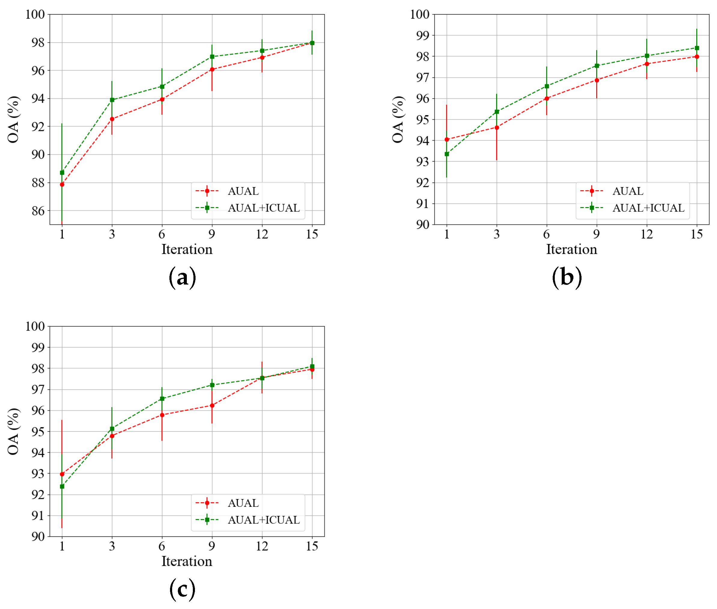
• We propose an active learning architecture based on inter-class uncertainty (ICUAL). By measuring the uncertainty of sample pairs, the instances located on both sides of the inter-class decision boundary are queried and sent to the training set. The classification ability of the model can be optimized by strengthening the inter-class feature comparison.

2. Related Work

2.1. Siamese Network

The siamese network consists of a dual branch with shared parameters. Since the input of the siamese network is a sample pair, constructed by two samples, the training data set can be augmented through sample pairing. The siamese network can learn differences between features by extracting the deep feature of a sample pair and judging the similarity with specific matching functions, which is called contrastive learning. The aim of the siamese network is to cluster intra-class samples and separate out samples of inter-class. Specifically, during the training process, when matched, the distance of a sample pair is reduced by the constructive loss function. If unmatched, the sample pair forces the loss function to increase the distance. The contrastive loss function of the siamese network is defined by:

$$\mathrm{loss}=\overline{\mathrm{y}}\ast {\mathrm{d}}^2+(1-\overline{\mathrm{y}})\ast {\max (\mathrm{margin}-\mathrm{d},0)}^2,$$

(1)

where $\overline{\mathrm{y}}$ indicates whether the sample pair belong to the same class or not. If two samples belong to the same class, $\overline{\mathrm{y}}=1$. Otherwise, $\overline{\mathrm{y}}=0$. $\mathrm{d}$ denotes the similarity distance between two sides of a sample pair. margin is the threshold that controls the loss of negative sample pairs. The traditional siamese network can only obtain the similarity between samples, which makes it difficult to perform the classification task. To integrate the siamese network and the classifier into an end-to-end framework, Cao [37] added a classification structure to the siamese network, calculating the loss of each individual sample and training the classifier. Xue [38] designed a lightweight siamese structure for feature fitting and fast classification.

2.2. Active Learning-Based DL Model

Active learning is an advanced strategy to obtain the most valuable samples through iterative queries for the model to effectively fine-tune. Active learning strategies have been widely used in the field of machine learning, such as breaking ties [39], normalized entropy [29], uncertainty sampling [40] and Margin sampling [41]. Since DL models are usually composed of CNN and classifiers, active learning can evaluate the uncertainty score by the posterior probability of sample categories that the deep learning model predicts and thereby select valuable samples. The combination of active learning and DL models has been studied for HSI classification. Specifically, Li [30] proposed a framework combining a multi-class-level uncertainty criterion with stacked auto-encoder. Cao [42] unified best-versus-second best (BvSB) [43] and CNN into a single framework, exploiting the powerful feature extraction capability of CNN as well as the effective labeling efficiency of active learning. Xue [44] designed a deep active learning method based on BvSB to measure the spatial uncertainty and information diversity of candidate samples.

3. Proposed Framework

In this section, we first explain the operation of ALSN and then explain the various parts of the framework. As shown in Figure 1, ALSN consists of the DLSN, AUAL and ICUAL. Firstly, the DLSN, which consists of a contrastive learning module and a classification module, is pre-trained by a few samples and sample pairs. The remaining samples and negative sample pairs together form the candidate pool. Then, the pre-trained DLSN uses the classification module to extract deep features of the candidate samples and output the probabilities that the candidate samples belong to each class. According to the class probability provided by the DLSN, AUAL actively queries the class-adversarial samples from the candidate pool into the training data set, which are used with pre-training samples to fine-tune the network. After AUAL, the newly labeled and previous training samples form the sample pairs. Positive sample pairs are directly sent to the training set, and negative sample pairs are sent to the candidate pool. The contrastive learning module fuses features of the negative sample pair and outputs the probability that the candidate sample pair belongs to a negative class. Next, ICUAL queries the negative sample pairs with inter-class uncertainty from the candidate pool, constructs the lightweight sample pair training set, and optimizes the model from both ends of the decision boundary through fine-tuning, which further enhances the classification ability of the DLSN.

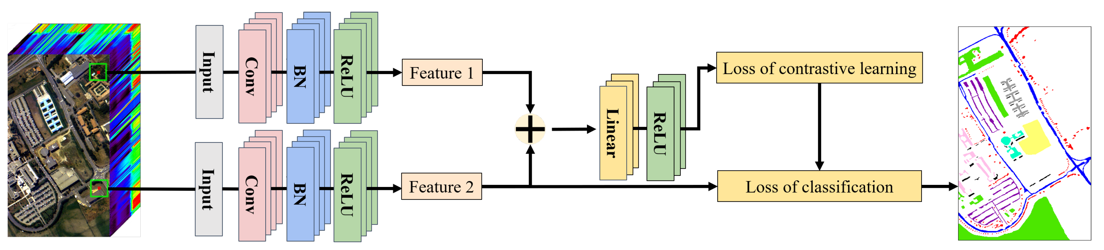
3.1. Dual Learning-Based Siamese Network

As shown in Figure 2, our proposed dual learning-based siamese network (DLSN) includes a contrastive learning module and a classification module. To facilitate the introduction of these two modules, we first introduce two training data formats of the model. The HSI dataset includes $\mathrm{C}$ categories of ground objects. We set $\mathrm{D}$ samples in each class as the training datasets. The training dataset of the $\mathrm{C}$th class could be represented as ${\mathrm{X}}_{\mathrm{C}}=[{\mathrm{x}}_{(\mathrm{C},1)},...,{\mathrm{x}}_{(\mathrm{C},\mathrm{D})}]$. The label of training samples could be denoted by ${\mathrm{Y}}_{\mathrm{C}}=[{\mathrm{y}}_{(\mathrm{C},1)},...,{\mathrm{y}}_{(\mathrm{C},\mathrm{D})}]$ and ${\mathrm{y}}_{(\mathrm{C},1)}=,...,={\mathrm{y}}_{(\mathrm{C},\mathrm{D})}$. Thus, the training data set of the classification module was $\mathrm{A}=[({\mathrm{X}}_1,{\mathrm{Y}}_1),...,({\mathrm{X}}_{\mathrm{C}},{\mathrm{Y}}_{\mathrm{C}})]$. For any two samples ${\mathrm{x}}_{\mathrm{i}}$ and ${\mathrm{x}}_{\mathrm{j}}$, $\mathrm{i},\mathrm{j}\in 1,...,\mathrm{C}\times \mathrm{D}$, a sample pair ${\mathrm{H}}_{\mathrm{ij}}=[{\mathrm{x}}_{\mathrm{i}},{\mathrm{x}}_{\mathrm{j}}]$ was constructed, which was the data set of the contrastive learning module. The label was formulated as below:

$$\mathbf{f}\left(\mathbf{x}\right)=\left\{\begin{array}{c}\hfill 0,{\mathrm{y}}_{\mathrm{i}}={\mathrm{y}}_{\mathrm{j}}\hfill \\ \hfill 1,{\mathrm{y}}_{\mathrm{i}}\ne {\mathrm{y}}_{\mathrm{j}}\hfill \end{array}\right.$$

(2)

In the contrastive learning module, we first used a two-branch DLSN with shared weight parameters to extract the features of sample ${\mathrm{x}}_{\mathrm{i}}$ and ${\mathrm{x}}_{\mathrm{j}}$ in the sample pair ${\mathrm{H}}_{\mathrm{ij}}$. Then, two sets of features h(${\mathrm{x}}_{\mathrm{i}}$) and h(${\mathrm{x}}_{\mathrm{i}}$) were fused as ${\mathrm{h}}_{\mathrm{ij}}$ and fed into the nonlinear projection layer [45] to obtain refined features of the sample pair. Finally, we used the binary classifier to match the probability of sample pairs. We used a binary cross-entropy loss function to partly adjust the network in this module, which is described as:

$$\mathrm{l}=-\overline{\mathrm{y}}\ast log\left(\widehat{\mathrm{y}}\right)-(1-\overline{\mathrm{y}})\ast log(1-\widehat{\mathrm{y}}),$$

(3)

where $\overline{\mathrm{y}}$ and $\widehat{\mathrm{y}}$ denote class probability and the label of a sample pair ${\mathrm{H}}_{\mathrm{ij}}$. During training, the module constantly contrasts the feature similarity of ${\mathrm{H}}_{\mathrm{ij}}$ to learn the ability of distinguishing the relationship feature between positive and negative sample pairs.

For the classification module, we used the DLSN trained by the contrastive learning module to extract the deep features from labeled training samples and we used multi-category cross-entropy loss for supervisory learning, represented as:

$$\mathrm{L}=-\sum _{\mathrm{k}=1}^{\mathrm{C}}{\mathrm{y}}_{\mathrm{k}}\ast log\left(\widetilde{{\mathrm{y}}_{\mathrm{k}}}\right),$$

(4)

where $\mathrm{C}$ represents the number of the category, $\mathrm{y}$ is the $\mathrm{k}$th label, and $\widetilde{{\mathrm{y}}_{\mathrm{k}}}$ is the probability of the $\mathrm{k}$th label the model predicts.

The detailed structure of DLSN is shown in

Table 1. Details of the dual learning-based siamese network (considering PaviaU dataset as an instance).

Layer	Output Shape	Output Shape	Layer
Input	(1,20,15,15) × 2	(1,20,15,15)	Input
Conv3d	(8,14,13,13) ×2	(8,14,13,13)	Conv3d
BatchNorm3d	(8,14,13,13) ×2	(8,14,13,13)	BatchNorm3d
ReLU	(8,14,13,13) ×2	(8,14,13,13)	ReLU
Conv3d	(16,10,11,11) ×2	(16,10,11,11)	Conv3d
BatchNorm3d	(16,10,11,11) ×2	(16,10,11,11)	BatchNorm3d
ReLU	(16,10,11,11) ×2	(16,10,11,11)	ReLU
Conv3d	(32,8,9,9) ×2	(32,8,9,9)	Conv3d
BatchNorm3d	(32,8,9,9) ×2	(32,8,9,9)	BatchNorm3d
ReLU	(32,8,9,9) ×2	(32,8,9,9)	ReLU
Conv2d	(64,7,7) ×2	(64,7,7)	Conv2d
BatchNorm2d	(64,7,7) ×2	(64,7,7)	BatchNorm2d
ReLU	(64,7,7) ×2	(64,7,7)	ReLU
AdaptiveAvgPool2d	(64,4,4) ×2	(64,4,4)	AdaptiveAvgPool2d
Linear	(1024) ×2	(1024)	Linear
Concatenate	(2048)	-	Concatenate
Linear	(512)	(512)	Linear
ReLU	(512)	(512)	ReLU
Linear	(128)	(9)	Linear
ReLU	(128)	-	-
Linear	(32)	-	-
ReLU	(32)	-	-
Linear	(2)	-	-
	Contrastive learning module	Classification module

. The encoder includes a 3D convolution layer, 2D convolution layer, batch normalization layer and ReLU layer. The adaptive global pooling layer was adopted to further down sample the features. Then, in the contrastive learning module, the nonlinear projection head is composed of a fully connected layer and ReLU layer, designed to learn fused sample pair feature representation. Finally, the two modules all use the fully connected layer for classification.

Since each sample forms multiple pairs with other samples, abundant sample pairs heavily increase the training cost of the DLSN. Further, negative sample pairs outnumbered the positive. If there are no constraints on the model, DLSN pays serious attention to inter-class distance, while ignoring the convergence of intra-class distance. So we adopted a random selection strategy [38] to choose a few equal proportions of positive and negative sample pairs for training during each epoch. The random selection strategy was proved to ensure a balance of positive and negative sample pairs and accelerated the training speed.

3.2. Adversarial Uncertainty-Based Active Learning (AUAL)

The common goal of the siamese network and of active learning is to acquire stronger classification ability with the least labeling cost. Therefore, we believe that the combination of these two methods is meaningful for dealing with limited labeled samples problem. However, if the siamese network, with high classification ability, is taken as the backbone network of active learning, it is a problem as to whether the active learning method, based on posterior probability, can query the really valuable samples under the requirement of minimal labeling cost.

Based on this problem, we propose a method called adversarial uncertainty-based active learning (AUAL) to accurately query valuable samples under small sample problems. First, the posterior probability-based active learning method measures the uncertainty of samples through the backbone network, aiming at the confusion degree of samples in the feature space. We believe that a sample set queried in this way can still be subdivided into class-adversarial samples and class-chaotic samples. Class-adversarial samples are those that have conflicting probability of being classified into a limited number of categories during the classification process. These samples are usually located close to the decision boundaries of specific groups of categories. The class-chaotic samples refer to the instances with relatively balanced and generally low probability of being classified into various categories in the classification process. These samples are located at multiple sets of the edge of decision boundaries. Class-adversarial samples and class-chaotic samples can be queried as Equations (5) and (6):

$$\mathrm{argmin}[(1-{\mathrm{P}}_{\mathrm{first}}\ast {\mathrm{P}}_{\mathrm{second}})\ast ({\mathrm{P}}_{\mathrm{first}}-{\mathrm{P}}_{\mathrm{second}}+\mathrm{q})],$$

(5)

$$\mathrm{argmin}[({\mathrm{P}}_{\mathrm{first}}\ast {\mathrm{P}}_{\mathrm{second}})\ast ({\mathrm{P}}_{\mathrm{first}}-{\mathrm{P}}_{\mathrm{second}}+\mathrm{q})],$$

(6)

where ${\mathrm{P}}_{\mathrm{first}}$ stands for the best posterior probability of category and ${\mathrm{P}}_{\mathrm{second}}$ denotes the second-largest posterior probability of category. $\mathrm{q}$ is a constant used to prevent invalid calculation due to the same ${\mathrm{P}}_{\mathrm{first}}$ and ${\mathrm{P}}_{\mathrm{second}}$.

We believe that in the limited labeled samples problem, it is more valuable to provide class-adversarial samples for the backbone network with high classification ability. Training these samples can precisely fine-tune some missing decision boundaries and help the model learn a more complete data distribution. Class-chaotic samples are more suitable for the backbone network with low classification ability. By training these samples, multiple decision boundaries can be optimized simultaneously with less labeling costs.

Therefore, in our framework, DLSN is set as the backbone network, and  Formula (5) is iteratively used to query class-adversarial samples for labeling. After these samples are sent to the data set, the classification ability of the DLSN can be improved by fine-tuning at minimal labeling cost.

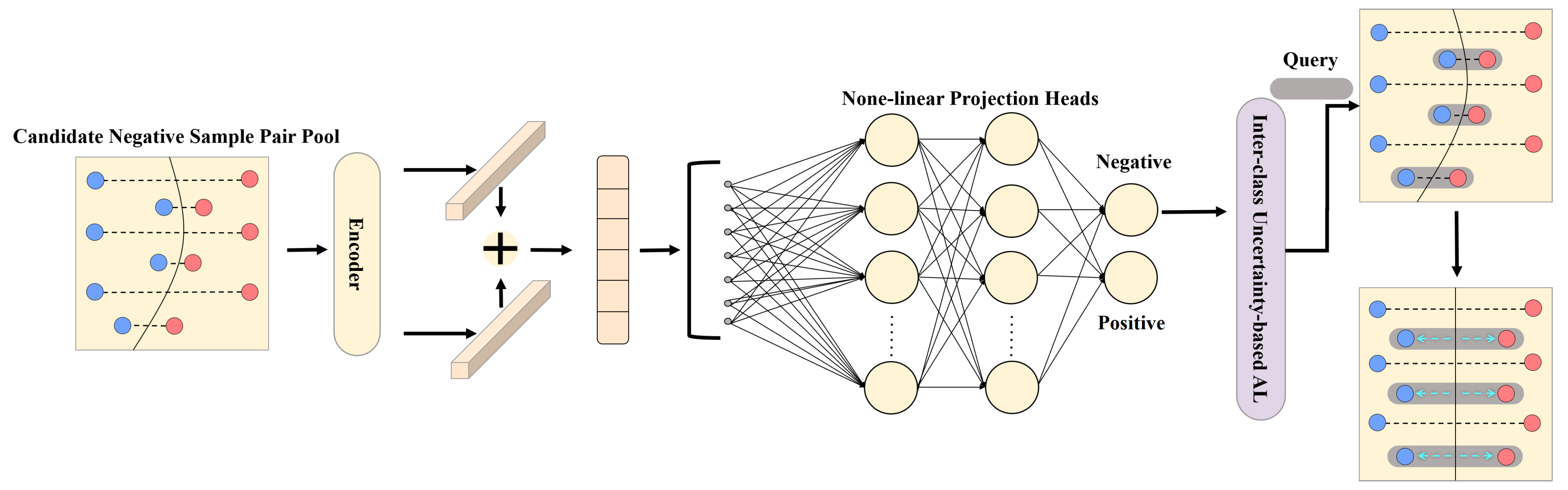
3.3. Inter-Class Uncertainty-Based Active Learning (ICUAL)

In our framework, as the iteration progresses, new instances and previous samples form many negative sample pairs. There are many redundant instances that cannot provide effective features in these negative sample pairs. Therefore, we believe that by eliminating abundant invalid negative sample pairs and mining valuable instances, the model can accurately learn and distinguish the characteristics of inter-class relationship, and avoid underfitting. However, traditional active learning, based on posteriori probability, queries individual samples at the decision boundary. This method essentially queries the samples that unilaterally change the decision boundary by fine-tuning the feature encoder, which is not suitable to measure inter-class relationships. Inspired by the siamese network, we propose an active learning architecture based on inter-class uncertainty (ICUAL). By actively querying inter-class instances located at both ends of the decision boundary, we constructed a lightweight sample pair data set. The decision boundary could be purposely optimized by simultaneously strengthening the inter-class feature contrast on both sides of the decision boundary.

Specifically, in the pre-training process of the model, we only used all the positive sample pairs and the same number of negative sample pairs as the positive sample pairs to construct a pre-training data set, and the rest were sent to the candidate pool. Meanwhile, we paired the samples queried in each iteration with the training samples. The positive sample pairs were added to the training data set, and the negative sample pairs were added to the candidate pool. After each iteration of AUAL, the ICUAL started in time. Through purposeful iterative screening, we formed a small and precise sample pair training set, providing more valuable inter-class features for the model. It is worth mentioning that, at the end of contrastive learning module we designed there is a binary classifier, which provides a metric method of inter-class uncertainty. As shown in the Figure 3, we input the entire sample pair candidate pool, and the features of each unit in the sample pair fused after being extracted by the encoder. After multiple layers of nonlinear projection, the classifier output the classification probability of negative instances. We used the following formula to query instances that lay on the binary classification boundary:

$$\mathrm{argmin}\left[\right|0.5-{\mathrm{P}}_{\mathrm{Negative}}\left({\mathrm{H}}_{\mathrm{ij}}\right)\left|\right],$$

(7)

where ${\mathrm{P}}_{\mathrm{Negative}}$ indicates the probability of negative class. In this way, all positive sample pairs and selected negative sample pairs could be regarded as a small and refined training set. Under the premise of using positive sample pairs to ensure intra-class aggregation, the samples on both sides of the decision boundary were fully mined. The decision boundary was jointly optimized through precise fine-tuning of negative sample pairs composed of bilateral samples. At the same time, in order to achieve the coordination of training cost and classification accuracy, we conducted multiple rounds of ICUAL after each iteration of AUAL. By means of dynamic supplementation, DLSN could be prevented from losing valuable features. Therefore, by training these valuable negative sample pairs, the ability of the contrastive learning module to distinguish inter-class or intra-class features could be greatly improved, thereby enhancing the ability of the DLSN to capture the global feature distribution and make classification decisions.

Synthesizing the above methods, the pseudo code of the ALSN algorithm can be seen in Algorithm 1.

Algorithm 1 Active Learning-driven Siamese Network (ALSN) for Hyperspectral Image Classification.

1: Input: D_1    training sample set D_2    training sample pair set U_1    candidate unlabeled sample set U_2    candidate labeled sample pair set N_1    the number of samples to query N_2    the number of negative sample pairs to query R_1    max iteration to query samples R_2    max round to query sample pairs 2: Initialization: k = 0, i = 0   3: for k = 0 to R1-1 do   4:    calculate class probability of candidate sample in $\mathrm{U}\_1$   5:    select $\mathrm{N}\_1$ instances from $\mathrm{U}\_1$ by AUAL   6:    update $\mathrm{D}\_1$=$\mathrm{D}\_1$⋃$\mathrm{N}\_1$ and $\mathrm{U}\_1$=$\mathrm{U}\_1\backslash \mathrm{N}\_1$   7:    fine-tune the DLSN   8:    for i = 0 to R2-1 do   9:         calculate class probability of candidate sample pair in $\mathrm{U}\_2$   10:       select $\mathrm{N}\_2$ instances from $\mathrm{U}\_2$ by ICUAL   11:       update $\mathrm{D}\_2$=$\mathrm{D}\_2$⋃$\mathrm{N}\_2$ and $\mathrm{U}\_2$=$\mathrm{U}\_2\backslash \mathrm{N}\_2$   12:       fine-tune the DLSN   13:    end for   14: end for   15: Output: Make predictions for the testing data with the trained DLSN.

4. Experiments

4.1. Data Sets

• University of Pavia (PaviaU): The PaviaU HSI was captured on July 8 by ROSIS. The wavelength of this HSI was in the range of 0.43–0.86 µm, which was divided into 103 Spectral bands. The image sizes of PaviaU were 610 pixels high and 340 pixels wide, with 1.3m spatial resolution. The false-color sample image of PaviaU and the ground-truth classification map are shown in Figure 4a,b. A total of 9 different classes and 42,776 labeled samples were contained in the ground-truth map. Specific class information of ground objects can be seen in

  Table 2. Classes of ground objects with number of labeled samples for three data sets.

  PaviaU			Salinas			YRD
  Class	Object	Number	Class	Object	Number	Class	Object	Number
  	Asphalt	6613		Broccoli green weeds 1	20,093		Reed	310
  	Meadows	18,649		Broccoli green weeds 22	3726		Spartina alterniflora	187
  	Gravel	2099		Fallow	1976		Salt filter pond	247
  	Trees	3064		Fallow rough plow	1394		Salt evaporation pond	300
  	Painted metal sheets	1345		Fallow smooth	2678		Dry pond	140
  	Bare soil	5029		Stubble	3959		Tamarisk	127
  	Bitumen	1330		Celery	3579		Salt pan	306
  	Self-Blocking Bricks	3682		Grapes untrained	11,271		Seepweed	218
  	Shadows	947		Soil vineyard develop	6203		River	584
  				Corn senesced green weeds	3278		Sea	4694
  				Lettuce romaine 4wk	1068		Mudbank	14
  				Lettuce romaine 5wk	1927		Tidal creek	67
  				Lettuce romaine 6wk	916		Fallow land	459
  				Lettuce romaine 7wk	1070		Ecological restoration pond	310
  				Vineyard untrained	7268		Robinia	111
  				Vineyard vertical trellis	1807		Fishpond	124
  							Pit pond	128
  							Building	398
  							Bare land	87
  							Paddyfield	508
  							Cotton	332
  							Soybean	71
  							Corn	103
  Total		42,776			54,129			9825

  .
• Salinas: The second dataset was Salinas HSI, which was acquired in Salinas Valley, California by AVIRIS. The wavelength of this HSI was in the range of 0.4–2.5 µm, which was divided into 204 Spectral bands. The image sizes of Salinas were 512 pixels high and 217 pixels wide. This data set was characterized by a spatial resolution of 3.7 m. The false-color sample image of the Salinas and the ground-truth classification map are shown in Figure 5a,b. A total of 16 different classes and 54,129 labeled samples were contained in the ground-truth map. Specific class information of ground objects can be seen in Table 2.
• Yellow River Delta (YRD): The third data set was YRD, which was recently captured over the Yellow River Delta wetland in China by ZY-02D AHSI. The wavelength of this HSI was in the range of 0.395–2.501 µm, which was divided into 119 Spectral bands. The image sizes of YRD were 1147 pixels high and 1600 pixels wide. This data set was characterized by a spatial resolution of 30 m. The false-color sample image of the YRD and the ground-truth classification map are shown in Figure 6a,b. A total of 23 different classes and 9825 labeled samples were contained in the ground-truth map. Specific class information of ground objects can be seen in Table 2.

4.2. Experimental Settings

• For hyperparameters: For DLSN, the learning rate parameters of training samples and sample pairs were initialized with 0.001. The reduced dimension after PCA for the three datasets were 20, 40, 40. The patch size was set as 15 × 15. The above settings were discussed in the hyperparameter analysis. Respectively, we set the weight decay of the classification module to 0.00005 during training. The batch size and training epoch were set as 64 and 40. Since there are two stages of pre-training and fine-tuning in ALSN, we set 20 epochs for pre-training, and 10 and 15 epochs for fine-tuning after AUAL and ICUAL.
• For sample selection: There were two sampling selection strategies in this paper. For naive DLSN, we randomly selected 10 samples per class for hyperparameter analysis and 19 samples per class for comparison analysis. For ALSN, we set 15 iterations for ablation analysis. We randomly selected 10 samples per class for pre-training. Then 9, 16 and 23 samples were individually queried during each active learning iteration for the three datasets. In addition, the number of negative sample pairs selected by ICUAL were discussed in ablation analysis.
• For performance comparison: Three-dimensional convolutional neural network (3-D CNN) [17], spectral-spatial residual network (SSRN) [46], spectral-spatial unified network (SSUN) [47], similarity-based deep metric model (S-DMM) [34] and deep active learning (CNN–AL–MRF) [42] were adopted to be compared with our proposed DLSN and ALSN. The five methods included three commonly used DL models, one advanced few-shot learning model, and one advanced deep active learning model.
• Experiment environment and Indicators: We used PyTorch 1.71 with Intel Core i5 (10,300 H) CPU GeForce RTX 2060 (6 GB) and 16 GB random access memory to perform a series of experiments. All experiments were performed independently and the average results of ten runs were saved. Meanwhile, we adopted overall accuracy (OA), average accuracy (AA), and Kappa coefficient ($\kappa$) to evaluate the experimental results. Moreover, train time (s) and test time (s) were used for complexity comparison.

4.3. Hyperparameter Analysis

In this part, we used 10 samples per class and all sample pairs as the data set. During each epoch, with the aim of analyzing the impacts of learning rate on DLSN, the learning rate of sample and sample pair were set in [$1\times {10}^{-5}$, $5\times {10}^{-5}$, $1\times {10}^{-4}$, $5\times {10}^{-4}$, $1\times {10}^{-3}$, $5\times {10}^{-3}$, $1\times {10}^{-2}$]. The evolution curve of OA, influenced by the learning rate of sample and sample pair, is demonstrated in Figure 7a,b. From the curve change results, OA was generally higher than the others when the two learning rates were set to $1\times {10}^{-3}$. Therefore, the learning rates of DLSN were fixed as $1\times {10}^{-3}$.

With the aim of analyzing the influence on the number of PCs on OA, we set this parameter in the range of [10, 20, ⋯, 100, 103] in PaviaU, [10, 20, ⋯, 200, 204] in Salinas, and [10, 20, ⋯, 110, 119] in YRD. The evolution curve of OA influenced by this parameter is demonstrated in Figure 7c. Specifically, for PaviaU, DLSN could get the highest OA when the number of PCs were retained as 20, so we retained 20 PCs for this data set. Likewise, for the other two data sets, we set the number of PCs as 40.

Regarding the input sample size, we set the patch size in the range of [9, 11, 13, 15, 17, 19]. The evolution curve of OA influenced by this parameter is demonstrated in Figure 7d. As can be seen, with the increase of the patch size, the OA of classification gradually improved. When the patch size was set to 15 × 15, the OA of DLSN basically stopped increasing, so the patch size was determined to be 15 × 15.

4.4. Ablation Analysis

4.4.1. Adversarial Uncertainty-Based Active Learning (AUAL)

In this experiment, we used 10 samples per class and all sample pairs as a pre-training data set. A total of 15 iterations of each active learning strategy were conducted for the three above HSI datasets. The backbone network used was DLSN. The experiment using this method was repeated 10 times.

We first compared the labeling value of class-chaotic samples and class-adversarial samples in the small sample problem. We visualized the classification probability of class-chaotic sample and class-adversarial sample in

Table 3. The classification probability obtained by DLSN for class-chaotic and class-adversarial samples (considering PaviaU dataset as an instance).

Class-Chaotic Sample		Class-Adversarial Sample
Input	Class5: 0.018	input	Class5: 0.000
Class1: 0.269	Class6: 0.104	Class1: 0.000	Class6: 0.000
Class2: 0.265	Class7: 0.003	Class2: 0.012	Class7: 0.000
Class3: 0.108	Class8: 0.042	Class3: 0.488	Class8: 0.488
Class4: 0.068	Class9: 0.123	Class4: 0.003	Class9: 0.009

. The probability of each category of the class-chaotic sample was relatively average and low. Marking and training such samples could optimize multiple decision boundaries simultaneously. Meanwhile, the probabilities of class 3 and 8 of class-adversarial sample were similar and far higher than that of other categories. Labeling and training of such samples could improve the classification ability of these two categories purposefully.

Then, we compared the impact of labeling these two types of samples on the classification accuracy of the model, namely, adversarial uncertainty-based active learning (AUAL) and chaotic uncertainty-based active learning (CUAL). We also added three classical active learning methods for comparison, namely, BvSB, entropy measure (EP) [43] and random sampling (RS). We report the evolution of OA values for iterations [1, 3, 6, 9, 12, 15] in Figure 8.

As can be seen, under the condition that there were only a few labeling costs in each iteration, the improvement effect of querying class-adversarial samples on model classification ability was continuously higher than that of class-chaotic samples. This confirmed our idea that in the small sample problem, the backbone network with higher classification accuracy needs to learn the missing distribution features more by supplementing the class-adversarial samples. In addition, compared with the other three active learning methods, AUAL could achieve the best performance, which verified the rationality of AUAL.

4.4.2. Inter-Class Uncertainty-Based Active Learning (ICUAL)

To verify the effectiveness of ALSN with ICUAL, we first analyzed the number of negative instances and iterations required by ICUAL after the first iteration of AUAL. We chose 10 samples per class, all the positive sample pairs and a few negative sample pairs equal to the number of the positive as the pre-training data set. After choosing samples by AUAL, we first fine-tuned the DLSN and then set the rounds of ICUAL from [1, 2, 3, 4, 5]. The number of negative sample pairs were selected from [100, 200, 300, 400, 500]. The average OA are shown in Figure 9. Considering the classification accuracy, we set the optimal combination of [4, 200] for PaviaU, [2, 300] for Salinas and [2, 200] for YRD.

Then, we conducted the experiment with 15 iterations of ALSN to evaluate the superiority of ICUAL. As can be seen in Figure 10, with the combination of AUAL and ICUAL, DLSN achieved higher classification accuracy. The averaged OA of 9 iterations and total number of training sample pairs are summarized in

Table 4. Comparison of AUAL and AUAL + ICUAL after 9 iterations.

Data Sets	Method	OA	Num of Pairs
PaviaU	AUAL	96.06 ± 1.56	14,535
	AUAL+ICUAL	96.97 ± 0.87	8884
Salinas	AUAL	96.87 ± 0.87	46,056
	AUAL+ICUAL	97.55 ± 0.74	10,267
YRD	AUAL	96.23 ± 0.87	95,266
	AUAL+ICUAL	97.20 ± 0.28	7660

Note: Num of pairs represents the total number of sample pairs that participated in the training.

. The OA of ALSN with AUAL and ICUAL exceeded ALSN with naive AUAL on three data sets. Furthermore, the number of pairs for training, when using AUAL and ICUAL, was much smaller than whenusing naive AUAL. We believe that this was because AUAL provided a huge sample pair set, which was full of a large number of contradictory or invalid inter class features. Therefore, DLSN with high classification ability would not only fail to really learn useful knowledge in the training process, but also encounter over-fitting. From the perspective of active learning, ICUAL queries the samples at both ends of the decision boundary and sends them into the training set in the form of negative sample pairs. This not only reduces the redundancy of the sample pair, but also optimizes the classifier by comparing the features at both ends of the decision boundary.

4.5. Classification Results

In order to validate the superior effects of DLSN and ALSN, we compared the classification performance of different methods when 9 iterations for ALSN were conducted. The parameters of ALSN were consistent with the results in the ablation analysis. For none active learning methods, 19 samples per class were randomly selected as the training set. In total, 171, 304 and 437 labeled samples in the three datasets were respectively used for comparison.

According to the

Table 5. Classification accuracy (%) for PaviaU dataset (9 iterations for AL methods and 19 labeled samples per class for other methods).

Class	3-DCNN [17]	SSRN [46]	SSUN [47]	S-DMM [34]	CNN-AL-MRF [42]	DLSN (Ours)	ALSN (Ours)
1	87.76 ± 3.95	93.67 ± 10.09	84.25 ± 2.78	93.30 ± 3.91	86.91 ± 4.57	90.75 ± 8.12	94.45 ± 4.76
2	93.09 ± 1.37	93.47 ± 5.83	80.38 ± 6.21	88.62 ± 4.74	92.85 ± 3.99	93.55 ± 2.53	99.35 ± 0.47
3	52.90 ± 7.36	72.86 ± 12.39	72.08 ± 8.23	92.06 ± 5.08	78.53 ± 13.66	89.66 ± 5.27	87.3 ± 7.13
4	70.84 ± 6.02	84.60 ± 15.21	97.53 ± 1.81	96.88 ± 2.19	94.07 ± 1.71	93.98 ± 2.6	93.83 ± 5.39
5	99.08 ± 1.61	99.98 ± 0.03	99.19 ± 1.20	100.00 ± 0.00	100.00 ± 0.00	99.95 ± 0.11	98.22 ± 3.66
6	64.57 ± 12.07	84.49 ± 9.10	84.14 ± 8.49	95.52 ± 3.53	95.64 ± 3.24	94.19 ± 11.23	98.51 ± 1.42
7	59.41 ± 9.41	82.97 ± 5.83	89.44 ± 3.79	99.74 ± 0.14	97.33 ± 1.65	99.02 ± 1.56	98.75 ± 1.16
8	66.40 ± 3.33	82.72 ± 4.31	91.65 ± 2.79	90.42 ± 5.07	85.71 ± 5.99	84.14 ± 9.23	94.04 ± 4.13
9	69.08 ± 3.35	91.99 ± 7.82	99.61 ± 0.30	99.97 ± 0.04	97.95 ± 0.83	98.46 ± 1.17	98.39 ± 1.42
OA (%)	78.01 ± 3.35	88.58 ± 3.76	84.49 ± 2.09	92.02 ± 2.71	91.50 ± 1.50	92.70 ± 2.00	96.97 ± 0.87
AA (%)	73.68 ± 2.82	87.42 ± 3.57	88.70 ± 1.34	95.17 ± 1.55	92.11 ± 0.94	93.75 ± 1.97	95.87 ± 1.02
$\kappa \times$100	71.92 ± 3.80	84.93 ± 5.06	80.07 ± 2.45	89.66 ± 3.39	88.88 ± 1.88	90.41 ± 2.66	95.99 ± 1.15

, ALSN acquired the best OA of 96.97 ± 0.87% on PaviaU data set, which was 4.27–18.96% higher than the other DL methods. For specific accuracy of each class, ALSN obtained the best results for 4 classes, including asphalt, meadows, bare soil and self-blocking bricks. In addition, ALSN also achieved great performance in terms of AA and KAPPA compared to others. For other methods, CNN-AL-MRF had good classification results for most of the ground objects, but poor performance in the third class, which was only correctly classified 78.53% of ground objects. S-DMM obtained the OA of 92.02 ± 2.71% with a good classification ability in the classes of few ground objects. We believe that S-DMM is equipped with a specific design to learn the complete feature distribution under small training set scenario, which is suitable for few-shot learning naturally. For 3-D CNN, SSRN and SSUN, the classification accuracies of these three methods were relatively low. The classification maps are shown in Figure 11. As can be seen, ALSN could accurately classify the samples with complex surrounding ground objects.

According to

Table 6. Classification accuracy (%) for Salinas dataset (9 iterations for AL methods and 19 labeled samples per class for other methods).

Class	3-D CNN [17]	SSRN [46]	SSUN [47]	S-DMM [34]	CNN-AL-MRF [42]	DLSN (Ours)	ALSN (Ours)
1	99.91 ± 0.17	100.00 ± 0.00	96.52 ± 3.39	99.84 ± 0.28	99.88 ± 0.24	99.75 ± 0.61	98.94 ± 1.99
2	99.17 ± 0.39	99.96 ± 0.07	95.14 ± 3.68	99.78 ± 0.19	98.96 ± 2.40	99.29 ± 1.63	99.88 ± 0.31
3	93.07 ± 3.02	97.37 ± 1.55	98.46 ± 1.48	99.11 ± 2.06	98.68 ± 1.63	99.95 ± 0.10	99.77 ± 0.54
4	97.76 ± 1.66	98.16 ± 1.49	99.91 ± 0.20	99.83 ± 0.20	97.51 ± 3.16	99.81 ± 0.18	99.14 ± 1.21
5	95.36 ± 2.68	97.91 ± 1.38	98.54 ± 0.53	99.42 ± 0.36	94.54 ± 3.13	98.41 ± 1.83	98.16 ± 1.61
6	99.74 ± 0.40	100.00 ± 0.0	99.72 ± 0.37	99.94 ± 0.08	99.24 ± 0.82	99.79 ± 0.23	99.49 ± 1.06
7	98.48 ± 1.67	99.97 ± 0.05	96.80 ± 2.39	99.95 ± 0.05	99.57 ± 0.53	99.95 ± 0.07	99.49 ± 1.06
8	81.9 ± 2.74	86.78 ± 2.08	79.66 ± 7.52	82.02 ± 8.19	77.70 ± 9.18	87.33 ± 4.02	95.02 ± 3.63
9	98.18 ± 1.34	99.61 ± 0.30	99.55 ± 0.48	99.63 ± 0.59	99.89 ± 0.19	99.67 ± 0.36	99.92 ± 0.17
10	91.11 ± 3.10	93.85 ± 3.94	95.06 ± 2.60	96.17 ± 1.30	91.30 ± 3.70	96.33 ± 1.94	98.07 ± 2.04
11	95.36 ± 3.20	97.82 ± 2.67	98.40 ± 0.71	99.53 ± 0.72	99.41 ± 0.53	99.93 ± 0.10	99.44 ± 0.89
12	90.88 ± 3.73	99.18 ± 0.99	99.53 ± 0.98	100.00 ± 0.00	99.72 ± 0.34	98.83 ± 3.01	99.44 ± 1.16
13	90.80 ± 3.53	99.83 ± 0.27	99.38 ± 0.52	99.76 ± 0.23	98.62 ± 3.14	99.46 ± 0.58	98.52 ± 2.82
14	85.57 ± 6.95	95.33 ± 5.03	98.56 ± 1.40	99.39 ± 0.43	99.31 ± 0.52	96.78 ± 6.12	97.64 ± 4.58
15	64.21 ± 6.02	77.38 ± 4.09	83.32 ± 10.42	81.85 ± 5.32	78.33 ± 7.93	87.43 ± 9.92	92.92 ± 4.54
16	99.12 ± 0.74	99.31 ± 1.75	97.13 ± 2.05	98.87 ± 4.55	97.14 ± 3.01	98.66 ± 1.10	99.23 ± 0.46
OA (%)	88.54 ± 1.34	93.23 ± 0.59	92.14 ± 0.94	93.37 ± 1.39	91.20 ± 0.93	95.08 ± 1.21	97.55 ± 0.74
AA (%)	92.54 ± 0.85	96.40 ± 0.57	95.98 ± 0.67	97.19 ± 0.41	95.61 ± 0.45	97.59 ± 0.76	98.47 ± 0.52
$\kappa \times$100	87.27 ± 1.47	92.47 ± 0.65	91.27 ± 1.04	92.62 ± 1.53	90.23 ± 1.01	94.52 ± 1.35	97.27 ± 0.82

, ALSN exceeded other methods with the best classification effect on Salinas data set. Specifically, ALSN acquired an OA of 97.55 ± 0.74%, which was 2.47–9.01% better than the other models. Meanwhile, ALSN also achieved great performance on AA and KAPPA. For specific accuracy of each class, ALSN obtained the best results for 4 classes, including grapes untrained, soil vineyard, corn senesced green weeds and vineyard untrained. In addition, DLSN achieved the second-highest classification accuracy after ALSN and maintained high accuracy for the test results of each class. For CNN-AL-MRF, although equipped by the active learning method, the backbone network of this method was not suitable for the small sample problem, resulting in 6.35% lower than the OA of ALSN. The classification maps are shown in Figure 12. Compared to the other methods, the whole classification map predicted by ALSN retained more detail with less noise.

For the YRD data set, according to

Table 7. Classification accuracy (%) for YRD dataset (9 iterations for AL methods and 19 labeled samples per class for other methods).

Class	3-D CNN [17]	SSRN [46]	SSUN [47]	S-DMM [34]	CNN-AL-MRF [42]	DLSN (Ours)	ALSN (Ours)
1	83.53 ± 4.05	93.70 ± 5.70	68.14 ± 7.43	84.22 ± 6.62	65.39 ± 13.13	87.01 ± 5.33	84.43 ± 5.79
2	93.67 ± 6.41	99.51 ± 0.60	80.06 ± 5.87	98.57 ± 3.11	94.94 ± 4.21	95.36 ± 5.72	93.17 ± 4.83
3	98.74 ± 1.30	98.05 ± 3.90	93.68 ± 3.85	98.15 ± 5.24	98.89 ± 1.39	96.05 ± 6.13	97.52 ± 3.73
4	89.82 ± 6.48	99.02 ± 1.61	81.49 ± 6.68	97.79 ± 3.28	96.62 ± 6.30	98.97 ± 2.08	97.16 ± 3.64
5	90.75 ± 6.67	95.86 ± 7.06	86.78 ± 9.02	96.69 ± 3.30	96.06 ± 2.75	96.86 ± 3.66	95.86 ± 3.52
6	72.79 ± 6.74	83.08 ± 3.83	88.52 ± 4.08	95.09 ± 5.54	91.14 ± 4.36	92.50 ± 3.69	92.47 ± 3.32
7	96.17 ± 8.74	100.00 ± 0.00	96.27 ± 2.20	100.00 ± 0.07	96.01 ± 3.17	98.78 ± 2.05	99.0 ± 2.17
8	97.24 ± 2.26	97.79 ± 2.32	83.42 ± 5.66	98.94 ± 1.15	99.66 ± 0.49	96.18 ± 4.39	96.61 ± 3.63
9	98.87 ± 1.83	98.21 ± 3.31	99.42 ± 0.41	100.00 ± 0.0	100.00 ± 0.00	99.33 ± 0.82	99.54 ± 1.38
10	99.49 ± 0.51	99.93 ± 0.15	89.82 ± 2.75	94.30 ± 3.14	91.47 ± 3.60	93.69 ± 4.58	99.64 ± 0.35
11	86.08 ± 20.34	85.00 ± 30.00	92.86 ± 11.52	100.00 ± 0.00	100.00 ± 0.00	94.29 ± 17.14	100.00 ± 0.0
12	34.57 ± 28.53	62.78 ± 36.85	88.54 ± 7.64	97.29 ± 2.80	92.22 ± 4.81	90.00 ± 6.31	85.83 ± 7.84
13	97.14 ± 2.28	95.21 ± 2.91	74.95 ± 3.54	98.68 ± 1.66	93.79 ± 4.81	92.32 ± 5.41	96.41 ± 6.06
14	73.70 ± 13.55	86.97 ± 15.37	74.09 ± 10.67	93.12 ± 5.66	80.77 ± 8.46	92.85 ± 5.06	91.87 ± 8.27
15	84.14 ± 10.81	90.77 ± 12.55	96.30 ± 3.80	100.00 ± 0.0	95.35 ± 5.01	100.00 ± 0.0	96.69 ± 6.07
16	65.22 ± 14.69	84.48 ± 16.12	90.00 ± 4.35	97.61 ± 3.44	91.32 ± 9.41	96.95 ± 3.99	98.4 ± 3.41
17	66.97 ± 30.15	84.45 ± 28.28	87.61 ± 8.77	95.32 ± 3.31	84.15 ± 5.09	97.61 ± 3.87	96.72 ± 2.5
18	97.48 ± 2.13	97.66 ± 1.98	58.28 ± 8.74	99.10 ± 1.05	91.91 ± 5.97	95.09 ± 4.44	93.98 ± 2.79
19	80.66 ± 15.14	81.73 ± 12.45	92.06 ± 6.97	100.00 ± 0.0	99.09 ± 1.31	97.79 ± 3.56	97.09 ± 3.95
20	92.42 ± 3.47	93.43 ± 4.31	92.17 ± 4.72	95.64 ± 1.97	87.68 ± 4.58	90.57 ± 6.56	93.27 ± 3.443
21	87.94 ± 6.88	95.61 ± 2.03	65.24 ± 4.89	91.62 ± 4.40	69.37 ± 6.72	90.42 ± 5.21	90.92 ± 3.74
22	63.92 ± 15.61	71.42 ± 17.61	98.46 ± 2.69	97.69 ± 2.95	95.17 ± 4.68	98.65 ± 2.44	94.18 ± 6.95
23	90.76 ± 6.91	99.05 ± 1.00	89.64 ± 4.58	98.69 ± 0.35	99.22 ± 0.51	97.62 ± 3.69	98.69 ± 1.07
OA (%)	90.88 ± 3.39	95.62 ± 2.95	86.35 ± 1.82	95.48 ± 1.49	90.91 ± 2.03	94.22 ± 2.65	97.20 ± 0.28
AA (%)	84.44 ± 2.72	91.03 ± 3.61	86.56 ± 1.37	96.89 ± 0.62	91.75 ± 0.79	95.17 ± 0.88	95.19 ± 0.50
$\kappa \times$100	88.08 ± 4.08	94.14 ± 3.80	82.02 ± 2.24	93.99 ± 1.94	88.10 ± 2.52	92.34 ± 3.37	96.24 ± 0.38

, ALSN achieved the best classification results in terms of OA and KAPPA, with OA of 97.20 ± 0.28%, which had a 6.32% (3-D CNN), 1.58% (SSRN), 10.85% (SSUN), 1.72% (S-DMM), 6.29% (CNN-AL-MRF) accuracy increase over OA. For specific accuracy of each class, ALSN obtained the best results for 2 classes. In addition, DLSN also obtained the highest classification accuracy of 4 classes. For specific accuracy of each class, S-DMM reached the greatest AA of 96.89 ± 0.62%. Figure 13 shows the whole classification maps. According to the results, ALSN and DLSN obtained more accurate results of ground feature distribution.

5. Discussion

5.1. Feature Separability Analysis

In order to demonstrate the effectiveness of our method for distinguishing inter-class and intra-class features, we used the same number of samples and iterations involved in the comparison experiment for training and reduced the high-dimensional features acquired by ALSN to two dimensions for separability visualization. As shown in Figure 14, for the PaviaU dataset, the features obtained by ALSN exhibited significantly improved feature separation to those obtained by naive DLSN. For example, trees and self-blocking bricks could maintain a certain distance from other classes while ensuring the intra-class aggregation. For the salinas dataset, it can be seen from the two-dimensional scatter plot that our proposed AUAL and ICUAL could also improve the separability of features. More obviously, after being enhanced by the two active learning methods, the model improved the intra-class aggregation and inter-class discrimination of grapes untrained and vineyard untrained noticeably. For the YRD dataset, most of the samples belonged to the sea class. Compared with DLSN, ALSN further reduced the intra-class distance of the sea class and increased the inter-class distance with other classes. The feature separability of the remaining classes was also improved.

5.2. Generalization Analysis

We compared the generalization performance of DLSN and ALSN with different deep learning methods on three common HSI datasets. For ALSN and CNN-AL-MRF, we conducted 15 iterations. For none active learning methods, 11–25 samples were randomly selected from each class as the training data set, and the remaining samples were sent to the testing data set. Figure 15 records the OA of all methods, as the number of iterations increased. As can be seen, the generalization performance of DLSN ranked among the top in different cases in the three data sets. ALSN achieved good improvement compared with DLSN and apparently acquired the best results under most circumstances for different iterations. Meanwhile, the generation performance of S-DMM on PaviaU and YRD data sets was higher than those of traditional DL models and CNN-AL-MRF. While CNN-AL-MRF combined active learning strategy, due to the poor classification ability of its backbone network, this method was unable to achieve great improvement of accuracy with less labeling cost. Therefore, We consider the prominent generalization performance of DLSN and ALSN demonstrate the effectiveness of our methods. We also believe the following factors led to the result. First, DLSN optimized the decision boundary by learning inter-class and intra-class features. Second, AUAL could query high-value samples for DLSN to fine-tune under the small sample problem, and further improved the model’s ability to fit the feature distribution. Finally, ICUAL eliminated a large number of redundant negative sample pairs, enabling DLSN to accurately capture useful inter-class information.

5.3. Time Complexity Analysis

To analyze the time complexity of ALSN, we used the same number of samples and iterations involved in the comparison experiment. The training and testing time are reported in

Table 8. Time cost (s) of different methods.

Data Sets	Metrics	3-D CNN [17]	SSRN [46]	SSUN [47]	S-DMM [34]	CNN-AL-MRF [42]	DLSN (Ours)	ALSN (Ours)
PaviaU	Training	17.25	85.72	13.29	3069	696.79	29.23	471.90
	Testing	5.72	25.21	3.59	95.91	10.98	12.83	14.38
Salinas	Training	30.45	306.96	20.51	3572	1292	69.8	907.45
	Testing	7.16	41.38	5.07	135.90	15.28	27.14	25.81
YRD	Training	39.92	144.63	31.96	33242	748.33	80.71	1268
	Testing	1.27	12.41	1.88	126.12	5.55	4.81	7.59

. As can be seen, compared to methods of limited labeled samples problem, classic deep learning methods, including 3-D CNN, SSRN and SSUN, all had less training time and testing time. This was because these methods only had two steps of sample feature extraction and classification, while methods of limited labeled samples problem require additional learning cost for few samples problems during the training period. S-DMM needs to divide the training data into support set and query set, which perform multiple feature matching calculations. DLSN has to use many neurons to fuse features or every sample pair. ALSN and CNN-AL-MRF constantly obtain new effective data in an iterative way, which has high time costs. Although the training cost of our method was higher than that of traditional DL models, it was comparable to other methods of limited labeled samples problem.

6. Conclusions

This paper proposes an active learning-driven siamese network (ALSN) for HSI classification. A dual learning-based siamese network (DLSN), consisting of a contrastive learning module and a classification module was first designed. Secondly, an active learning method based on adversarial uncertainty (AUAL) was proposed to query valuable samples with conflicting probability of being classified into different categories, providing DLSN with a few high-value samples for better classification. Finally, an active learning architecture, based on inter-class uncertainty (ICUAL), was designed. By querying negative sample pairs with uncertainty, lightweight training sets were constructed, which were used to optimize the classification capability from both ends of the decision boundary. Experiments on three common datasets demonstrated the effectiveness of our proposed DLSN, AUAL and ICUAL. At the same time, ablation experiments showed that iterative active query was more suitable for network learning feature distribution than random selection of quantitative training samples.

Although our proposed model has some advantages compared with other methods, there are still other shortcomings of ALSN that can be further studied: (1) Use of semi-supervised learning method for labeling the selected samples automatically; (2) Design more useful active learning-based measures to select informative samples.

References

1. Lacar, F.; Lewis, M.; Grierson, I. Use of hyperspectral imagery for mapping grape varieties in the Barossa Valley, South Australia. In Proceedings of the IEEE 2001 International Geoscience and Remote Sensing Symposium (Cat. No. 01CH37217), Sydney, NSW, Australia, 9–13 July 2001; IEEE: Piscataway, NJ, USA, 2001; Volume 6, pp. 2875–2877. [Google Scholar]
2. Matteoli, S.; Diani, M.; Corsini, G. A tutorial overview of anomaly detection in hyperspectral images. IEEE Aerosp. Electron. Syst. Mag. 2010, 25, 5–28. [Google Scholar] [CrossRef]
3. Foglini, F.; Angeletti, L.; Bracchi, V.; Chimienti, G.; Grande, V.; Hansen, I.M.; Meroni, A.N.; Marchese, F.; Mercorella, A.; Prampolini, M.; et al. Underwater Hyperspectral Imaging for seafloor and benthic habitat mapping. In Proceedings of the 2018 IEEE International Workshop on Metrology for the Sea; Learning to Measure Sea Health Parameters (MetroSea), Bari, Italy, 8–10 October 2018; pp. 201–205. [Google Scholar]
4. Zhang, L.; Zhang, L.; Du, B. Deep learning for remote sensing data: A technical tutorial on the state of the art. IEEE Geosci. Remote Sens. Mag. 2016, 4, 22–40. [Google Scholar] [CrossRef]
5. Zhu, X.X.; Tuia, D.; Mou, L.; Xia, G.S.; Zhang, L.; Xu, F.; Fraundorfer, F. Deep learning in remote sensing: A comprehensive review and list of resources. IEEE Geosci. Remote Sens. Mag. 2017, 5, 8–36. [Google Scholar] [CrossRef] [Green Version]
6. Paoletti, M.; Haut, J.; Plaza, J.; Plaza, A. Deep learning classifiers for hyperspectral imaging: A review. ISPRS J. Photogramm. Remote Sens. 2019, 158, 279–317. [Google Scholar] [CrossRef]
7. Chen, Y.; Lin, Z.; Zhao, X.; Wang, G.; Gu, Y. Deep learning-based classification of hyperspectral data. IEEE J. Sel. Top. Appl. Earth Obs. Remote Sens. 2014, 7, 2094–2107. [Google Scholar] [CrossRef]
8. Hu, W.; Huang, Y.; Wei, L.; Zhang, F.; Li, H. Deep convolutional neural networks for hyperspectral image classification. J. Sens. 2015, 2015, 258619. [Google Scholar] [CrossRef] [Green Version]
9. Mou, L.; Ghamisi, P.; Zhu, X.X. Deep recurrent neural networks for hyperspectral image classification. IEEE Trans. Geosci. Remote Sens. 2017, 55, 3639–3655. [Google Scholar] [CrossRef] [Green Version]
10. Chen, Y.; Zhao, X.; Jia, X. Spectral–spatial classification of hyperspectral data based on deep belief network. IEEE J. Sel. Top. Appl. Earth Obs. Remote Sens. 2015, 8, 2381–2392. [Google Scholar] [CrossRef]
11. Liu, Q.; Zhou, F.; Hang, R.; Yuan, X. Bidirectional-convolutional LSTM based spectral-spatial feature learning for hyperspectral image classification. Remote Sens. 2017, 9, 1330. [Google Scholar] [CrossRef] [Green Version]
12. Zhu, L.; Chen, Y.; Ghamisi, P.; Benediktsson, J.A. Generative adversarial networks for hyperspectral image classification. IEEE Trans. Geosci. Remote Sens. 2018, 56, 5046–5063. [Google Scholar] [CrossRef]
13. Yue, J.; Zhao, W.; Mao, S.; Liu, H. Spectral–spatial classification of hyperspectral images using deep convolutional neural networks. Remote Sens. Lett. 2015, 6, 468–477. [Google Scholar] [CrossRef]
14. Zhao, W.; Du, S. Spectral–spatial feature extraction for hyperspectral image classification: A dimension reduction and deep learning approach. IEEE Trans. Geosci. Remote Sens. 2016, 54, 4544–4554. [Google Scholar] [CrossRef]
15. Yue, J.; Mao, S.; Li, M. A deep learning framework for hyperspectral image classification using spatial pyramid pooling. Remote Sens. Lett. 2016, 7, 875–884. [Google Scholar] [CrossRef]
16. Mei, S.; Ji, J.; Geng, Y.; Zhang, Z.; Li, X.; Du, Q. Unsupervised spatial–spectral feature learning by 3D convolutional autoencoder for hyperspectral classification. IEEE Trans. Geosci. Remote Sens. 2019, 57, 6808–6820. [Google Scholar] [CrossRef]
17. Chen, Y.; Jiang, H.; Li, C.; Jia, X.; Ghamisi, P. Deep feature extraction and classification of hyperspectral images based on convolutional neural networks. IEEE Trans. Geosci. Remote Sens. 2016, 54, 6232–6251. [Google Scholar] [CrossRef] [Green Version]
18. Zhou, F.; Hang, R.; Li, J.; Zhang, X.; Xu, C. Spectral-Spatial Correlation Exploration for Hyperspectral Image Classification via Self-Mutual Attention Network. In IEEE Geoscience and Remote Sensing Letters; IEEE: Piscataway, NJ, USA, 2022. [Google Scholar]
19. Dong, Y.; Liu, Q.; Du, B.; Zhang, L. Weighted feature fusion of convolutional neural network and graph attention network for hyperspectral image classification. IEEE Trans. Image Process. 2022, 31, 1559–1572. [Google Scholar] [CrossRef] [PubMed]
20. Jia, S.; Jiang, S.; Lin, Z.; Li, N.; Xu, M.; Yu, S. A survey: Deep learning for hyperspectral image classification with few labeled samples. Neurocomputing 2021, 448, 179–204. [Google Scholar] [CrossRef]
21. Yang, J.; Zhao, Y.; Chan, J.C.W.; Yi, C. Hyperspectral image classification using two-channel deep convolutional neural network. In Proceedings of the 2016 IEEE International Geoscience and Remote Sensing Symposium (IGARSS), Beijing, China, 10–15 July 2016; IEEE: Piscataway, NJ, USA, 2016; pp. 5079–5082. [Google Scholar]
22. Sun, Y.; Li, J.; Wang, W.; Plaza, A.; Chen, Z. Active learning based autoencoder for hyperspectral imagery classification. In Proceedings of the 2016 IEEE International Geoscience and Remote Sensing Symposium (IGARSS), Beijing, China, 10–15 July 2016; IEEE: Piscataway, NJ, USA, 2016; pp. 469–472. [Google Scholar]
23. Liu, B.; Yu, X.; Yu, A.; Zhang, P.; Wan, G.; Wang, R. Deep few-shot learning for hyperspectral image classification. IEEE Trans. Geosci. Remote Sens. 2018, 57, 2290–2304. [Google Scholar] [CrossRef]
24. Yang, J.; Zhao, Y.Q.; Chan, J.C.W. Learning and transferring deep joint spectral–spatial features for hyperspectral classification. IEEE Trans. Geosci. Remote Sens. 2017, 55, 4729–4742. [Google Scholar] [CrossRef]
25. Lin, L.; Chen, C.; Yang, J.; Zhang, S. Deep transfer HSI classification method based on information measure and optimal neighborhood noise reduction. Electronics 2019, 8, 1112. [Google Scholar] [CrossRef]
26. Jiang, Y.; Li, Y.; Zhang, H. Hyperspectral image classification based on 3-D separable ResNet and transfer learning. IEEE Geosci. Remote Sens. Lett. 2019, 16, 1949–1953. [Google Scholar] [CrossRef]
27. Haut, J.M.; Paoletti, M.E.; Plaza, J.; Li, J.; Plaza, A. Active learning with convolutional neural networks for hyperspectral image classification using a new Bayesian approach. IEEE Trans. Geosci. Remote Sens. 2018, 56, 6440–6461. [Google Scholar] [CrossRef]
28. Liu, C.; Li, J.; He, L. Superpixel-based semisupervised active learning for hyperspectral image classification. IEEE J. Sel. Top. Appl. Earth Obs. Remote Sens. 2018, 12, 357–370. [Google Scholar] [CrossRef]
29. Tuia, D.; Ratle, F.; Pacifici, F.; Kanevski, M.F.; Emery, W.J. Active learning methods for remote sensing image classification. IEEE Trans. Geosci. Remote Sens. 2009, 47, 2218–2232. [Google Scholar] [CrossRef]
30. Li, J. Active learning for hyperspectral image classification with a stacked autoencoders based neural network. In Proceedings of the 2015 7th Workshop on Hyperspectral Image and Signal Processing: Evolution in Remote Sensing (WHISPERS), Tokyo, Japan, 2–5 June 2015; IEEE: Piscataway, NJ, USA, 2015; pp. 1–4. [Google Scholar]
31. Hu, J.; He, Z.; Li, J.; He, L.; Wang, Y. 3d-gabor inspired multiview active learning for spectral-spatial hyperspectral image classification. Remote Sens. 2018, 10, 1070. [Google Scholar] [CrossRef] [Green Version]
32. Zhao, S.; Li, W.; Du, Q.; Ran, Q. Hyperspectral classification based on siamese neural network using spectral-spatial feature. In Proceedings of the IGARSS 2018—2018 IEEE International Geoscience and Remote Sensing Symposium, Valencia, Spain, 22–27 July 2018; IEEE: Piscataway, NJ, USA, 2018; pp. 2567–2570. [Google Scholar]
33. Liu, Y.; Su, M.; Liu, L.; Li, C.; Peng, Y.; Hou, J.; Jiang, T. Deep residual prototype learning network for hyperspectral image classification. In Second Target Recognition and Artificial Intelligence Summit Forum; SPIE: Bellingham, WA, USA, 2020; Volume 11427, pp. 24–29. [Google Scholar]
34. Deng, B.; Jia, S.; Shi, D. Deep metric learning-based feature embedding for hyperspectral image classification. IEEE Trans. Geosci. Remote Sens. 2019, 58, 1422–1435. [Google Scholar] [CrossRef]
35. Deng, C.; Xue, Y.; Liu, X.; Li, C.; Tao, D. Active transfer learning network: A unified deep joint spectral–spatial feature learning model for hyperspectral image classification. IEEE Trans. Geosci. Remote Sens. 2018, 57, 1741–1754. [Google Scholar] [CrossRef] [Green Version]
36. Li, X.; Cao, Z.; Zhao, L.; Jiang, J. ALPN: Active-Learning-Based Prototypical Network for Few-Shot Hyperspectral Imagery Classification. IEEE Geosci. Remote Sens. Lett. 2021, 19, 1–5. [Google Scholar] [CrossRef]
37. Cao, Z.; Li, X.; Jiang, J.; Zhao, L. 3D convolutional siamese network for few-shot hyperspectral classification. J. Appl. Remote Sens. 2020, 14, 048504. [Google Scholar] [CrossRef]
38. Xue, Z.; Zhou, Y.; Du, P. S3Net: Spectral-Spatial Siamese Network for Few-Shot Hyperspectral Image Classification. In IEEE Transactions on Geoscience and Remote Sensing; IEEE: Piscataway, NJ, USA, 2022. [Google Scholar]
39. Luo, T.; Kramer, K.; Goldgof, D.B.; Hall, L.O.; Samson, S.; Remsen, A.; Hopkins, T.; Cohn, D. Active learning to recognize multiple types of plankton. J. Mach. Learn. Res. 2005, 6, 589–613. [Google Scholar]
40. Zhu, J.; Wang, H.; Tsou, B.K.; Ma, M. Active learning with sampling by uncertainty and density for data annotations. IEEE Trans. Audio Speech Lang. Process. 2009, 18, 1323–1331. [Google Scholar] [CrossRef]
41. Demir, B.; Persello, C.; Bruzzone, L. Batch-mode active-learning methods for the interactive classification of remote sensing images. IEEE Trans. Geosci. Remote Sens. 2010, 49, 1014–1031. [Google Scholar] [CrossRef] [Green Version]
42. Cao, X.; Yao, J.; Xu, Z.; Meng, D. Hyperspectral image classification with convolutional neural network and active learning. IEEE Trans. Geosci. Remote Sens. 2020, 58, 4604–4616. [Google Scholar] [CrossRef]
43. Joshi, A.J.; Porikli, F.; Papanikolopoulos, N. Multi-class active learning for image classification. In Proceedings of the 2009 IEEE Conference on Computer Vision and Pattern Recognition, Miami, FL, USA, 20–25 June 2009; IEEE: Piscataway, NJ, USA, 2009; pp. 2372–2379. [Google Scholar]
44. Xue, Z.; Zhou, S.; Zhao, P. Active learning improved by neighborhoods and superpixels for hyperspectral image classification. IEEE Geosci. Remote Sens. Lett. 2018, 15, 469–473. [Google Scholar] [CrossRef]
45. Chen, T.; Kornblith, S.; Norouzi, M.; Hinton, G. A simple framework for contrastive learning of visual representations. In Proceedings of the 37th International Conference on Machine Learning, Virtual Event, 13–18 July 2020; pp. 1597–1607. [Google Scholar]
46. Zhong, Z.; Li, J.; Luo, Z.; Chapman, M. Spectral–spatial residual network for hyperspectral image classification: A 3-D deep learning framework. IEEE Trans. Geosci. Remote Sens. 2017, 56, 847–858. [Google Scholar] [CrossRef]
47. Xu, Y.; Zhang, L.; Du, B.; Zhang, F. Spectral–spatial unified networks for hyperspectral image classification. IEEE Trans. Geosci. Remote Sens. 2018, 56, 5893–5909. [Google Scholar] [CrossRef]
Figure 1. Graphical illustration of active learning-driven siamese network (ALSN). First, the classification module of DLSN is used to actively query instances for fine-tuning and new sample pair construction. Second, the contrastive learning module is used to actively query instances with inter-class uncertainty from the negative sample pair pool for fine-tuning.
Remotesensing 15 00752 g001
Figure 2. Graphical illustration of dual learning-based siamese network (DLSN).
Remotesensing 15 00752 g002
Figure 3. Graphical illustration of inter-class uncertainty-based active learning (ICUAL).
Remotesensing 15 00752 g003
Figure 4. PaviaU. (a) False-color image, (b) Ground-truth map.
Remotesensing 15 00752 g004
Figure 5. Salinas. (a) False-color image, (b) Ground-truth map.
Remotesensing 15 00752 g005
Figure 6. Yellow River Delta. (a) False-color image, (b) Ground-truth map.
Remotesensing 15 00752 g006
Figure 7. Evolution of OA (%) as a function of (a) Learning rate of sample, (b) Learning rate of sample pair, (c) The number of PCs, (d) Patch size.
Remotesensing 15 00752 g007
Figure 8. Evolution of OA (%) obtained by different active learning strategies as a function of iteration. (a) PaviaU, (b) Salinas, (c) YRD.
Remotesensing 15 00752 g008
Figure 9. The impact of different ICUAL rounds and number of sample pairs on OA (after the first AUAL iteration). (a) PaviaU, (b) Salinas, (c) YRD.
Remotesensing 15 00752 g009
Figure 10. Evolution of OA (%) obtained by AUAL and AUAL+ICUAL as a function of iteration. (a) PaviaU, (b) Salinas, (c) YRD.
Remotesensing 15 00752 g010
Figure 11. Classification maps predicted by different methods for PaviaU dataset. (a) Ground-truth, (b) 3-D CNN (78.01%), (c) SSRN (88.58%), (d) SSUN (84.49%), (e) S-DMM (92.02%), (f) CNN-AL-MRF (91.50%), (g) DLSN (92.70%), (h) ALSN (96.97%).
Remotesensing 15 00752 g011
Figure 12. Classification maps predicted by different methods for Salinas dataset. (a) Ground-truth, (b) 3-D CNN (88.54 %), (c) SSRN (93.23%), (d) SSUN (92.14%), (e) S-DMM (93.37%), (f) CNN-AL-MRF (91.20%), (g) DLSN (95.08%), (h) ALSN (97.55%).
Remotesensing 15 00752 g012
Figure 13. Classification maps predicted by different methods for YRD dataset. (a) Ground-truth, (b) 3-D CNN (90.88%), (c) SSRN (95.62%), (d) SSUN (86.35%), (e) S-DMM (95.48%), (f) CNN-AL-MRF (90.91%), (g) DLSN (94.22%), (h) ALSN (97.20%).
Remotesensing 15 00752 g013
Figure 14. Feature separability for different methods in the three data sets. (a) DLSN, (b) ALSN with AUAL, and (c) ALSN with AUAL and ICUAL for PaviaU. (d) DLSN, (e) ALSN with AUAL, and (f) ALSN with AUAL and ICUAL for Salinas. (g) DLSN, (h)ALSN with AUAL, and (i) ALSN with AUAL and ICUAL for YRD.
Remotesensing 15 00752 g014
Figure 15. Evolution of OA obtained by different methods as a function of iteration. (a) PaivaU, (b) Salinas, (c) YRD.
Remotesensing 15 00752 g015