Negative Air Ion (NAI) Dynamics over Zhejiang Province, China, Based on Multivariate Remote Sensing Products

Abstract

Negative air ions (NAIs), which are known as the “air vitamin”, have been widely used as a measure of air cleanness. Field observation provides an alternative way to record site-level NAIs. However, these observations fail to capture the regional distribution of NAIs due to the limited number of sites. In this study, satellite-based bio-geophysical parameters from the climate, topography, air quality, vegetation, and anthropogenic intensity were used to estimate the daily NAIs with the Random Forest model (RF). In situ NAI observations over Zhejiang Province, China were incorporated into the model. Daily NAIs were averaged to capture the spatio-temporal distribution. The results showed that (1) the RF algorithm performed better than traditional regression analysis and the common BP neural network to generate regional NAIs at a spatial scale of 500 m over the larger scale, with an RMSE of 258.62, R² of 0.878 for model training, and R² of 0.732 for model testing; (2) in the variable importance measures (VIM) analysis, 87.96% of the NAI variance was caused by the elevation, aspect, slope, surface temperature, solar-induced chlorophyll fluorescence (SIF), relative humidity (RH), and the concentration of carbon monoxide (CO), while path analysis indicated that SIF was one of the most important factors affecting NAI concentration across the whole region; (3) NAI concentrations in 87.16% of the region were classified above grade III (>500 ions cm⁻³), which was able to meet the needs of human health maintenance; (4) the highest NAI concentration was distributed over the southwest of the Zhejiang Province, where forest land dominates. The lowest NAI concentration was mostly found in the northeast regions, where urban areas are well-developed; and (5) among different land types, the NAI concentrations were ranked as forest land > water bodies > barren > grassland > croplands > urban and built-up. Among different seasons, summer and winter have the highest and lowest NAIs, respectively. Our study provided a substantial reference for ecosystem services assessment in Zhejiang Province.

1. Introduction

Negative air ions (NAIs) are known as the air “vitamin”. High concentrations of NAIs will profoundly reduce air pollutants and defend against the physical illnesses caused by air pollution [1,2,3]. Thus, NAIs have been working as a key indicator in ecosystem services assessment during the past decades in China [4,5,6]. In previous studies, the dynamics and predictions of NAIs had been extensively investigated in order to realize accurate ecosystem services assessment [3,7,8].

Site-based NAI observations provide the most accurate way to record NAIs in a limited range within the core location of the site [2,9,10]. However, scarce monitoring sites have limited its regional application. Thus, more and more studies have tried to build up models to predict their spatio-temporal dynamics [5,6].

At the site scale, data-driven empirical models were the first attempts to predict NAI dynamics in the past decades [11,12,13]. Among the numerous influencing factors, climatic factors (such as air temperature, air moisture, radiation, wind speed, etc.) and air quality (such as PM_2.5, PM₁₀, SO_2, NO₂, etc.) are the most investigated [2,8,9]. In these studies, multi-parameter regression models were used to model the temporal dynamics of NAIs [10,14]. However, considering the limited site monitoring, the spatial distribution of NAIs is hard to predict [15]. At the regional scale, satellite-based bio-geophysical parameters such as the Normalized Difference Vegetation Index (NDVI), Gross Primary Productivity (GPP), Digital Elevation Model (DEM), air humidity, etc., were used to approach NAI regional distribution [16]. In these studies, simple regression models and semi-variogram models were adopted to predict the NAI spatial distribution with instantaneous NAI measurements [7,15,17]. In some other studies, these instantaneous data were also expanded via a geostatistical scheme, such as the variogram and Kriging method, to provide regional-scale NAIs according to the geostationary spatial variation [7,15,18]. Even though these site and regional scale models provide substantial reference for ecosystem services assessment [17,18], some drawbacks still needed to be solved.

Firstly, the data used to build NAI inversion models need to be refined [15]. Presently, studies with large amounts of long-term NAI monitoring data are still lacking. Even though a vast number of instantaneous point measurements might make up for the deficiency of site numbers, the lack of synchronization and temporal extensibility of these data perturb the feasibility of NAI modeling [11,15,17]. In addition, with more and more knowledge on NAI formation, plant functional traits such as transpiration, GPP, vegetation coverage, etc., have been progressively introduced into the NAI inversion [7,9,11]. However, these traits are alleged to indirectly interrupt NAI dynamics, which leads to weak NAI predictions [14]. Recently, photoelectric progress was argued to directly participate in NAI formations [10,14,17]. For example, NAIs were considered to be highly correlated to solar-induced chlorophyll fluorescence intensity (SIF), especially under higher PAR levels when vegetation photosynthesis was fully activated [10]. However, the spatial significance of the photosynthetic contribution to the regional NAI dynamics has been less assessed.

Secondly, the widely adopted simple empirical model fails to include multi-factor interactions [19]. The drawbacks of the statistical models mentioned above encourage the use of advanced data-driven machine-learning models, such as Random Forest and ANN models, which have special characteristics to simulate the unknown relationships among different parameters [7,13,20,21]. Machine-learning models can numerically formulate NAIs nonlinearly, solely based on historical data without requiring knowledge of the underlying physical processes. The continuous advancement of machine-learning methods over the last two decades demonstrates their suitability for object variables with an acceptable rate of outperforming conventional approaches [22].

In this study, the Random Forest (RF) machine-learning model was adopted to generate an NAI model based on site-based NAIs and observation multi-parameters. Furthermore, with the development of space technology, satellite-based models have been recorded as a possible way to model specific variables at a larger spatial scale [7,8,23,24]. Thus, the spatial information was also considered to realize the NAI inversion in this study. Furthermore, according to previous studies, meteorological factors such as radiation, water vapor, etc., and vegetation photosynthesis-related parameters provided the sources and energy for NAI formation [15,17]. Human activities and air pollutants are potentially quenching the existence of NAIs [2,7]. Topographic factors indirectly influence the NAIs via changing the vegetation and meteorological factors [17]. Thus, these five categories are incorporated into our NAI model.

As an important part of the large urban agglomeration in China [19], in the past decades, Zhejiang Province has experienced rapid urbanization and industrialization with economic growth, which has led to a large number of air-pollution-related health problems [25,26]. The rising demands for clean air have stimulated the need for NAI-related ecosystem services assessment. In this study, we used a large number of site-based NAI data that were continuously monitored to build the NAI inversion model. Meanwhile, satellite-based SIF was introduced in the model as an alternative to plant photoelectric progress. With the help of geographic information technologies, our study will realize the spatial–temporal modeling of regional NAI dynamics with higher resolutions in Zhejiang Province. We aimed to (1) evaluate the sensitivity of the bio-geophysical parameters to NAI dynamics, (2) generate satellite-based NAI estimation based on the RF model, and (3) explore the NAI dynamics across the Zhejiang Province, China.

2. Materials and Methods

2.1. Study Area

This study was conducted in Zhejiang Province, on the southeast coast of China (27.120–31.310°N, 118.010–123.100°E). It is one part of the Yangtze River Delta Economic Belt with a fast and high level of urbanization (Figure 1). A subtropical monsoon climate is dominant in this region, with a mean annual temperature of 15~18 °C and a mean annual precipitation of 1000~2000 mm. Seventy percent of the land surface is covered with hills and mountains. Forest and urban areas are distributed in the southwest and northeast of the study area (Figure 1).

2.2. Data Resources

2.2.1. Station-Based NAI Observations

Station-based NAI observations were collected from the Zhejiang Fresh Air Release System (http://223.4.64.202/zjqxkqfb/index, accessed on 4 January 2021). It provides NAI observations every 5 min over Zhejiang Province at 270 stations, among which 107 stations (including 76 sites in forests, 20 sites in urban and built-up areas, 9 sites in cropland, 1 site in wetland, and 1 site in grassland) with high-quality data collection during 2018–2020 were selected (Figure 1).

2.2.2. Remote Sensing Data

Five types of remote sensing data during 2018–2020 (including vegetation, topography, meteorological, human activity intensity, and air quality) were downloaded from the NAI observing sites (

Table 1. Data overview of the driving factors on NAI dynamics.

Data Sources		Factors	Temporal Resolution	Spatial Resolution	Unit	Classification
AgERA5		T	Daily	0.1°	K	Meteorological factors
		RH	Real-time	0.1°	/
		W	Daily	0.1°	m s−1
		RS	Daily	0.1°	J m−2 d−1
		VP	Daily	0.1°	hPa
		CC	Daily	0.1°	/
		DEWT	Daily	0.1°	K
MODIS	MYD16A2	ET	Eight-day	500 m	kg m−2 d−1
	MCD15A2H	FPAR	Eight-day	500 m	/
	MCD15A2H	LAI	Eight-day	500 m	/
	MYD17A2H	GPP	Eight-day	500 m	kg C m−2	Vegetation factor
GOSIF		SIF	Eight-day	0.05°	W m−2 μm−1 sr−1
SRTM		DEM	/	90 m	m	Topographic factor
		Slope	/	90 m	°
		Aspect	/	90 m	°
NPP/VIIRS		Lit	Monthly	1000 m	/	Intensity of human activity
China Environmental Monitoring Station		AQI	Hourly	/	/	Air quality factor
		PM2.5	Hourly	/	μg m−3
		PM10	Hourly	/	μg m−3
		SO2	Hourly	/	μg m−3
		NO2	Hourly	/	μg m−3
		CO	Hourly	/	mg m−3
		O3	Hourly	/	μg m−3

).

(1)

Vegetation datasets

In this study, photoelectric-related vegetation factors including the SIF, leaf area index (LAI), and gross primary productivity (GPP), were collected from the GOSIF and MODIS datasets, respectively (Table 1).

LAI, the fraction of absorbed photosynthetic active radiation (FPAR), and GPP datasets are available from MCD15A2H, MYD16A2, and MYD17A2H on NASA’s LAADSDAAC official website (https://ladsweb.modaps.eosdis.nasa.gov, accessed on 4 January 2021). These datasets have a spatial resolution of 500 m and a temporal resolution of 8 days. Only high-quality data were used based on the quality assurance (QA) layers in the MODIS datasets. Since these datasets may have unavoidable gaps caused by the cloud, GLASS products were used here to fill these gaps in the MODIS datasets.

The widely used GOSIF product was selected to provide regional-scale SIF (with a spatial resolution of 0.05°). These datasets were produced based on OCO-2, MODIS, and MERRA-2 datasets and were updated in December 2020. The GOSIF version 2 product was downloaded from the Global Ecology Data Repository (https://globalecology.unh.edu/data/GOSIF.html, accessed on 4 January 2021).

(2)

Meteorological datasets

Meteorological factors consist of evapotranspiration (ET), air temperature (T), relative humidity (RH), wind speed (W), solar radiation flux (R_S), vapor pressure deficit (VPD), cloud cover (CC), and dew point temperature (DEWT). These parameters were collected from the AgERA5 datasets. The data can be obtained from the Copernicus Climate Change Service (https://cds.climate.copernicus.eu/, accessed on 4 January 2021). The AgERA5 is meteorological re-analysis data based on hourly ECMWFERA5 surface data. Firstly, these datasets were aggregated to a daily temporal scale and resampled from 0.1° to 500 m.

(3)

Topographic datasets

Topographic parameters include the digital elevation model (DEM), slope, and aspect. These data were collected from the SRTM datasets, which were produced by the cooperation between NASA, the Department of Defense’s National Mapping Agency (NIMA), and space agencies in Germany and Italy. The DEM datasets were downloaded from the Geospatial Data Cloud Platform of the Computer Network Information Center of the Chinese Academy of Sciences (http://www.gscloud.cn, accessed on 4 January 2021).

(4)

Human activity intensity

Human activity intensity is represented by nighttime light radiation intensity (Lit). The Lit data were collected from the NPP/VIIRS datasets. NPP/VIIRS is the nighttime light data obtained by the visible light infrared imaging radiometer carried by the US National Polar Orbiting Cooperation Satellite. Since nighttime lights do not change much in a short period of time, this study uses monthly nighttime light data from 2020 with a spatial resolution of 1000 m, which are downloaded from the official website of the Earth Observation Group (EOG) (https://payneinstitute.mines.edu/eog/, accessed on 4 January 2021). Negative values were removed to improve the data quantity. In this paper, the mask-denoising method was used to preprocess the raw data. Firstly, negative values in the original data were replaced with 0 values. Secondly, the stable light data of DMSP in 2013, which was the closest to the date of the NPP/VIIRS data, was selected to form a mask (pixels with DN values greater than 0 in the DMSP image were assigned a value of 1). Finally, the mask data were multiplied by NPP /VIIRS data to achieve the purpose of denoising.

(5)

Air quality data

Air quality includes air quality index (AQI) and pollutant (PM_2.5, PM₁₀, SO₂, NO₂, CO, O₃) concentrations. These data were collected from China Environmental Monitoring Station. The air quality data selected in this paper can be downloaded from https://quotsoft.net/air/ (accessed on 4 December 2020). To match with the monitoring data of the NAI stations, the data were interpolated into raster data by using the Kernel Interpolation with Barriers (KIB) method. In this paper, 62 sites in Zhejiang Province and 108 surrounding sites were selected to obtain accurate interpolation results (Figure 1). Outliers were removed from the original site data, and the hourly data were calculated as daily averages.

In addition, we also downloaded the data product MCD12Q1 (2019) with a spatial resolution of 500 m to better analyze NAI concentration differences under different land-use types. The LC_Typel dataset of MCD12Q1 refers to the International Geosphere-Biosphere Programme (IGBP) global vegetation classification method to classify land cover. Referring to the National Classification Standard of Land Use Status (GB/T 2101-2017), this paper further combined the land-use types of Zhejiang Province into forests, urban and built-up areas, cropland, wetland, barren, and grassland.

Since multivariate remote sensing datasets have different spatial and temporal resolutions, we resampled the data to 500 m to unify the spatial resolution. In order to match NAI site data (daily mean data), the hourly air quality data with outliers removed were calculated as daily mean data. Since vegetation, terrain, and human activity intensity usually are stable in a short period of time, data from corresponding periods were directly used to simulate NAI concentrations.

2.3. Modelling

2.3.1. Random Forest

The Random Forest algorithm combines a series of independent regression trees by selecting random samples and features [27]. By generating a set of weak learners based on a bootstrap of the data, the algorithm converges to an optimal solution while avoiding issues related to CARTs and parametric statistics. In this paper, the Random Forest algorithm in the Matlab environment (v2016) was used to model the relationship between the 23 environmental variables and site-specific NAI measurements across the Zhejiang Province. Ninety percent of these data were used for model training, and the rest were used for model testing.

In the training procedure, each tree was built on a random subset of the original data (with replacements). Three parameters were optimized and named N_trees, M_try, _and Min_leaf. The first parameter presented the number of trees in the forest. M_try is the number of feature variables selected randomly for each decision split, and it was always set to one-third of the total number of variables for regression by default. As for Min_leaf, it defined the minimum number of observations per tree leaf and its default value was 5.

The modeling workflow is exhibited in Figure 2. During the training process, N_trees were identified according to the change in OOB.Error, and values of Min_leaf and M_try were ensured and combined with the grid search according to the determination coefficient (R²), root mean square error (RMSE), and bias obtained by ten-fold cross-validation. The model error decreased when N_trees increased to a certain level, and Min_leaf and M_try were influenced mutually. Considering the training time, the optimal parameter combination was chosen based on the training samples, and the model of validation samples and test samples were evaluated.

The relevant calculation formulas are as follows:

$${\mathrm{R}}_{\mathrm{C}}=\left|\frac{{\mathrm{X}}_{\mathrm{n}}-{\mathrm{X}}_{\mathrm{n}-1}}{{\mathrm{X}}_{\mathrm{n}-1}}\right|$$

(1)

where R_C represents the rate of change in the OOB.Error, X is OOB.Error, and n is the number of trees.

$${\mathrm{R}}^2={{\displaystyle \sum }}_{\mathrm{i}=1}^{\mathrm{n}}{\left(\widehat{{\mathrm{y}}_{\mathrm{i}}}-\overline{{\mathrm{y}}_{\mathrm{i}}}\right)}^2/{{\displaystyle \sum }}_{\mathrm{i}=1}^{\mathrm{n}}{\left({\mathrm{y}}_{\mathrm{i}}-\overline{{\mathrm{y}}_{\mathrm{i}}}\right)}^2$$

(2)

$$\mathrm{RMSE}=\sqrt{\frac{1}{\mathrm{n}}{{\displaystyle \sum }}_{\mathrm{i}=1}^{\mathrm{n}}{\left(\widehat{{\mathrm{y}}_{\mathrm{i}}}-{\mathrm{y}}_{\mathrm{i}}\right)}^2}$$

(3)

$$\mathrm{Bias}=\overline{\widehat{{\mathrm{y}}_{\mathrm{i}}}}-\overline{{\mathrm{y}}_{\mathrm{i}}}$$

(4)

where $\hat{\mathrm{y}}$ is the predicted value, y is the measured value, $\overline{\hat{\mathrm{y}}}$ is the mean of the predicted value, $\overline{\mathrm{y}}$ is the mean of the measured value, and n is the number of samples in the validation set.

Variable importance measures (VIM) performed from the RF algorithm made it possible to explore the weight of each input variable. For any variable, feature importance measures the increase in prediction error. The VIM metric is computed for each tree, then averaged and divided by the standard deviation of the entire ensemble. In this paper, 23 feature variables are ranked based on their feature importance score.

2.3.2. Path Analysis

In our study, path analysis was performed to determine the influence of multiple factors on NAI variations. Based on the pre-ranking of all the 23 feature variables mentioned above, the most related ten variables were extracted to conduct the path analysis. We assumed that the terrain factors are mainly applied to the NAI variation via disturbing the environmental heterogeneity spatially, which further shifts the NAIs. We used path analysis to determine the significant direct and indirect pathways through which the factors affected the NAIs. The path analysis was performed using the software package AMOS v21.0.

2.3.3. Spatio-Temporal Variation Analysis

Like other geographic phenomena, the spatial distribution of NAI concentrations is spatially correlated. In this paper, the spatial autocorrelation analysis of NAI was carried out by the global Moran’s index (Moran’s I) and local Moran’s I. The global Moran’s I is generally between −1 and 1. The local Moran’s index is used to identify the regional spatial auto-correlation of NAI. The calculations are shown below:

$$\mathrm{Global}\mathrm{Moran}’\mathrm{s}\mathrm{I}=\frac{{{\displaystyle \sum }}_{\mathrm{i}=1}^{\mathrm{n}}{{\displaystyle \sum }}_{\mathrm{j}=1}^{\mathrm{n}}{\mathrm{W}}_{\mathrm{ij}}\left({\mathrm{NAI}}_{\mathrm{i}}-\overline{\mathrm{NAI}}\right)\left({\mathrm{NAI}}_{\mathrm{j}}-\overline{\mathrm{NAI}}\right)}{{\mathrm{S}}^2{{\displaystyle \sum }}_{\mathrm{i}=1}^{\mathrm{n}}{{\displaystyle \sum }}_{\mathrm{j}=1}^{\mathrm{n}}{\mathrm{W}}_{\mathrm{ij}}}$$

(5)

$$\mathrm{Local}\mathrm{Moran}’\mathrm{s}\mathrm{I}=\frac{\left({\mathrm{NAI}}_{\mathrm{i}}-\overline{\mathrm{NAI}}\right)}{{\mathrm{S}}^2}{{\displaystyle \sum }}_{\mathrm{j}=1}^{\mathrm{n}}{\mathrm{W}}_{\mathrm{ij}}\left({\mathrm{NAI}}_{\mathrm{j}}-\overline{\mathrm{NAI}}\right)$$

(6)

where NAI_i and NAI_j are the NAI concentrations at i and j over the region, $\overline{\mathrm{NAI}}$ and S² are the mean and variance of NAI concentrations, W_ij is the spatial weight matrix, and n is the sample size.

3. Results

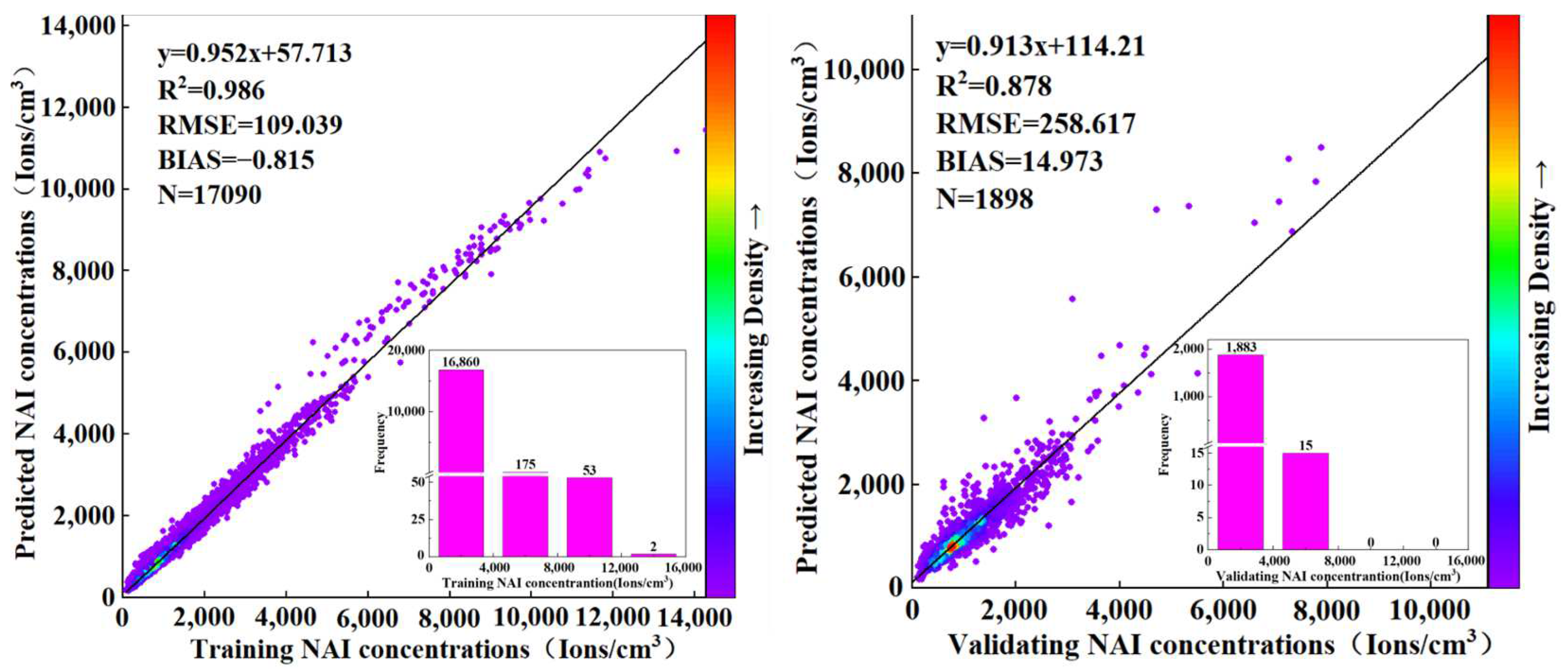
3.1. Model Performance

As shown in Figure 3, OOB.Error decreased rapidly with increased N_trees. When N_trees increased to 63, the OOB.Error started to be stable. Thus, N_trees was set to 63, and values of Min_leaf and M_try were located at 1~3 and 6~23, respectively. According to the following grid search (Figure 4), when Min_leaf = 1 and M_try = 10, the average R² obtained from ten-fold cross-validation was the largest (0.901) and the average RMSE was the smallest (279.456) (Figure 4).

Models were built based on “optimal” parameters and training samples, and model training and validation were also performed (Figure 5). In the model training process, R², RMSE, and bias for the model were 0.986, 109.039, ions cm⁻³, and 0.815 ions cm⁻³, respectively. In the validation process, R² = 0.878, RMSE = 258.617 ions cm⁻³, and bias = 14.973 ions cm⁻³, respectively. The efficiency of the model was evaluated for NAI > 4000 ions cm⁻³, and the R² and bias reached 0.68 and 321.90 respectively. These results proved an excellent model performance to be applied regionally.

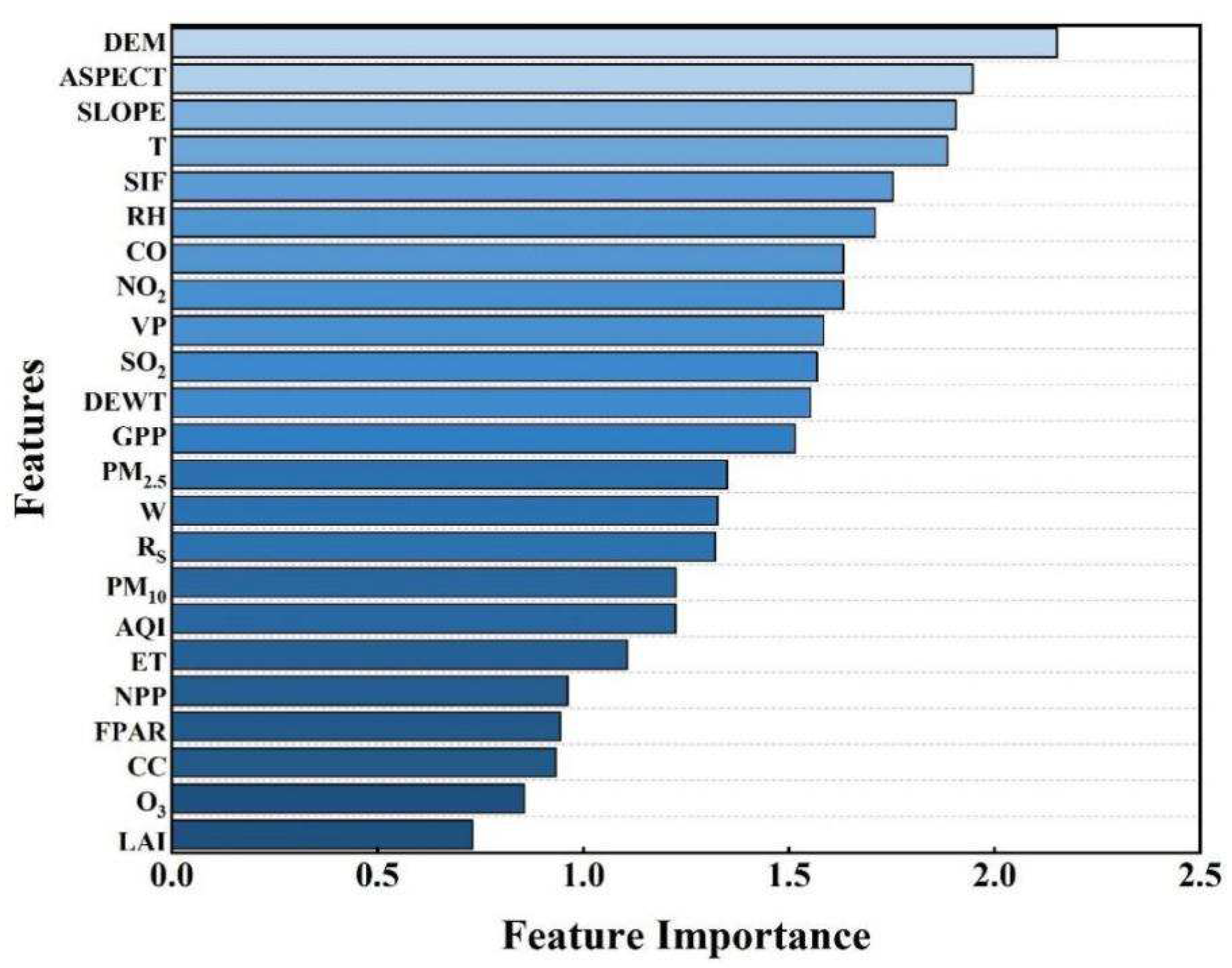
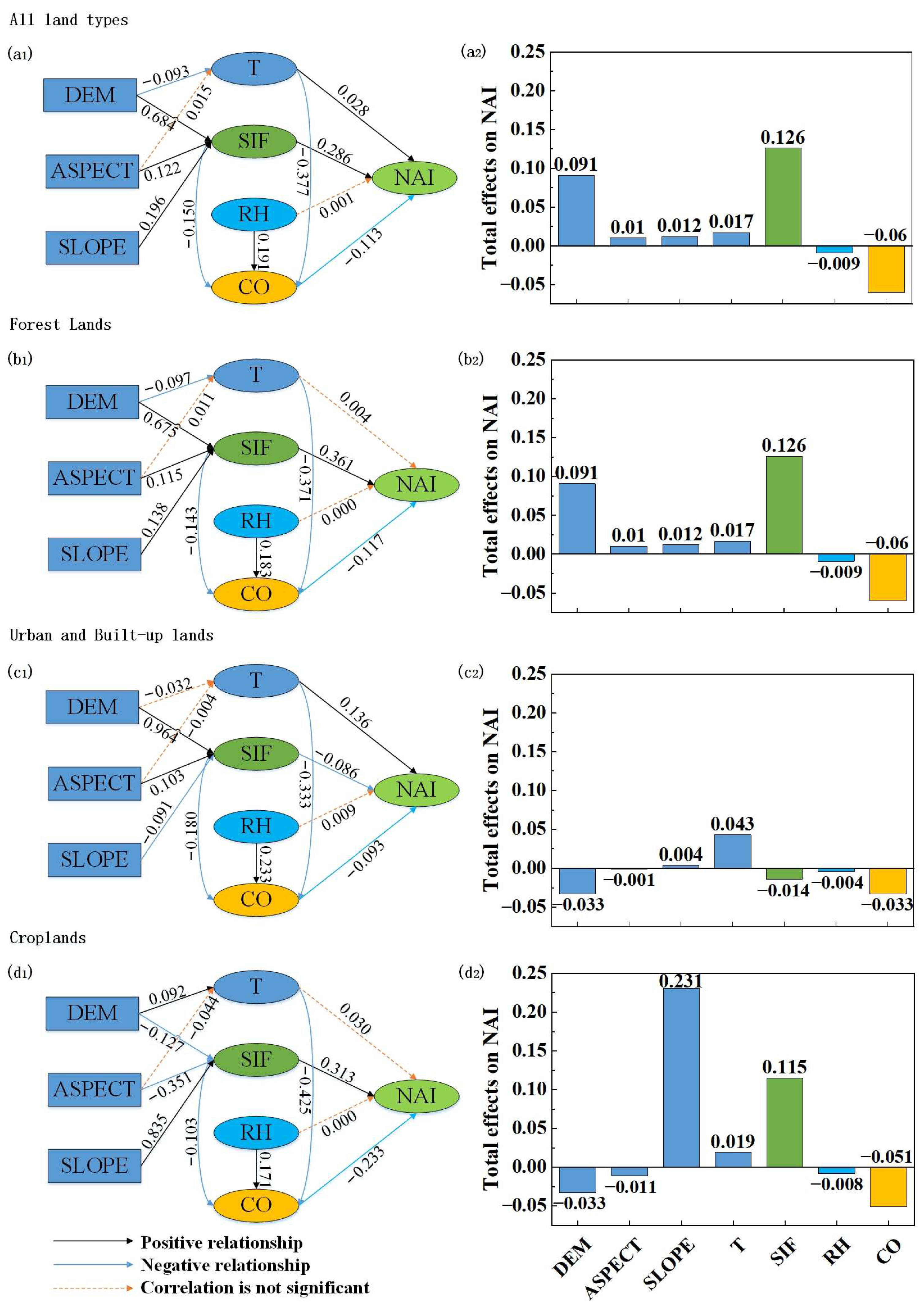
3.2. Driving Factors Determination

Ten featured variables with the greatest impact had been ranked in the RF model (Figure 6). These variables included topographic factors (DEM, aspect, slope), meteorological factors (T, Rh, VP), vegetation factors (SIF), and air quality factors (CO, NO₂, SO₂), among which the importance of SIF followed the DEM, aspect, slope, and T (Figure 6), which indicated the necessity to incorporate vegetation photosynthesis into the NAI model spatio-temporally.

In the path analysis, when all land types were considered, the path model for the NAI values explained 77.65% of their variance (df = 9, F = 18.57, RMSE = 0.054) (Figure 7a₁). The positive effects of T and SIF and the adverse effects of CO on the NAIs were the combinations of direct and indirect effects. The indirect effects of DEM on the NAI were mediated by SIF and T, which led to the positive effects of DEM on the NAIs (Figure 7a₂). The indirect effects of slope and aspect on the NAIs were mediated by SIF, which also led to positive effects on the NAIs (Figure 7a₂).

Similar to all land types, the model under forest land, urban and built-up land, and cropland also presented a good prediction with 84.23%, 71.23%, and 75.57% explanation for NAI variances. Furthermore, the direct and indirect effects of terrain features were quite similar to that of all land types for forest land (Figure 7b₁), which also produced a positive effect on NAIs. The direct and indirect effects for urban and building land and cropland tended to be different from that under all land types, especially for cropland, whose DEM influenced the NAI via the mediation of T and SIF, producing negative effects (Figure 7d₁,d₂). Meanwhile, slope had extraordinarily higher contributions to NAIs on cropland than the other land types (Figure 7d₂).

SIF was one of the most important factors affecting NAI concentration (except for urban and built-up land). In forest land and cropland, the total contribution of SIF to NAIs was 0.126 and 0.115, respectively. CO was another important factor affecting NAI concentration, which was mainly negatively correlated with NAIs, while T, SIF, and RH affected NAIs through CO. In all land types, the direct effect of RH on NAI was not significant. In addition, on construction land, the total contribution of T and CO to the NAI concentration was the largest (0.043 and, −0.033, respectively), and SIF was not the main factor affecting NAIs.

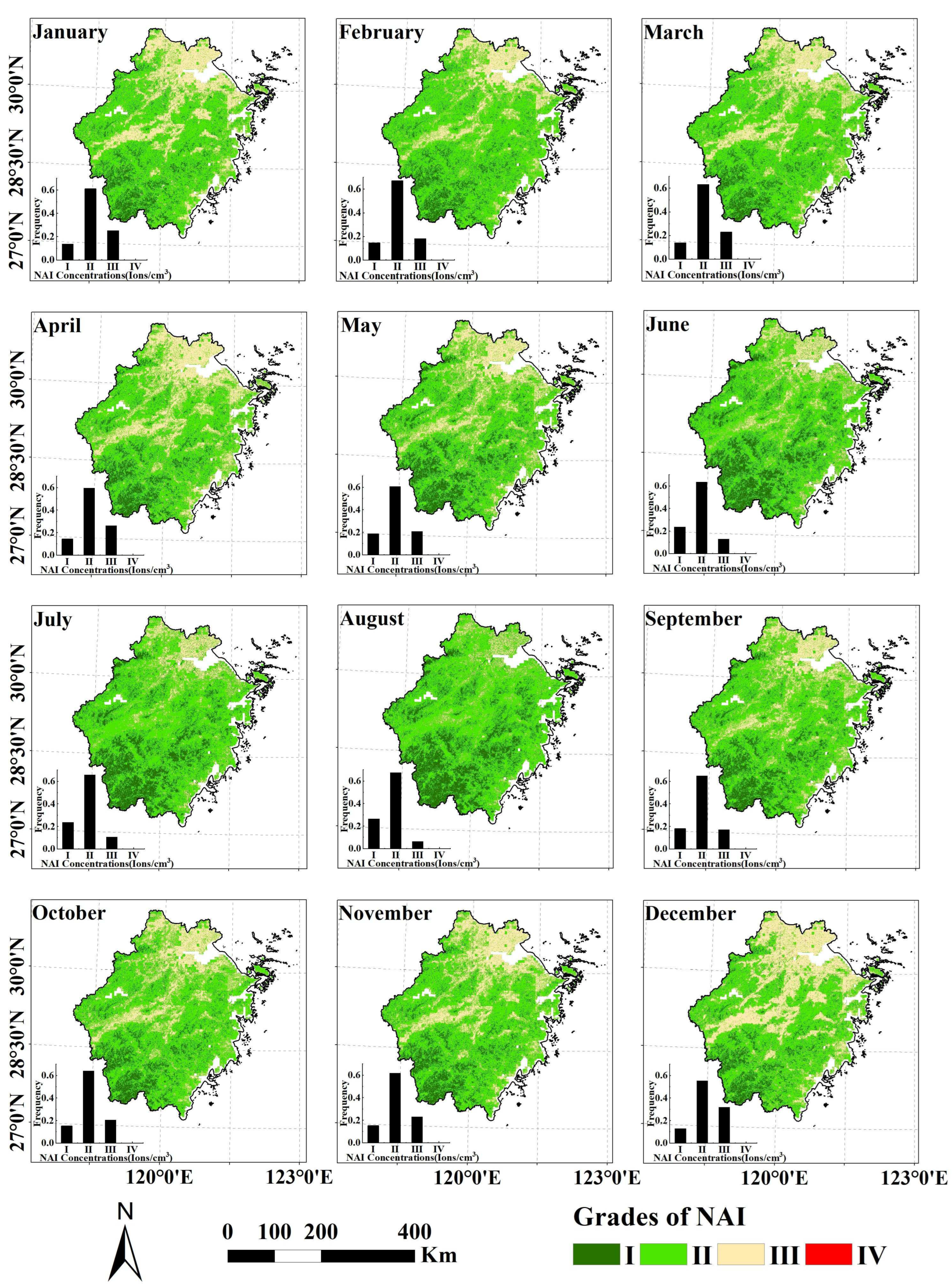
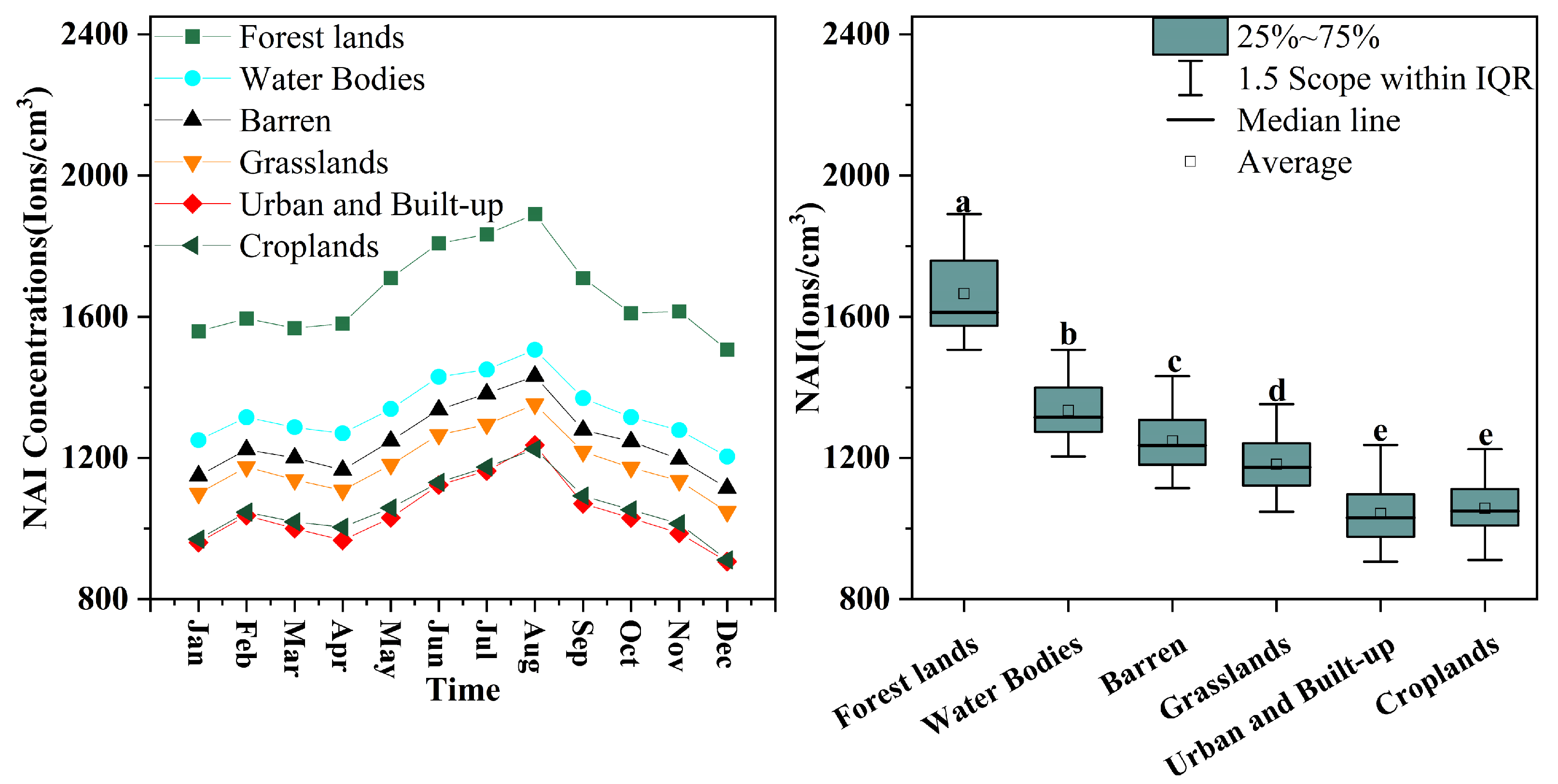
3.3. Characteristics of the NAI Temporal and Spatial Distribution

In this study, an RF model was developed to estimate the spatio-temporal distribution of NAIs in Zhejiang Province during 2020. The mean NAI concentration in Zhejiang Province in 2020 was 1550 ions cm⁻³, which ranged from the lowest value of 296 ions cm⁻³ to the highest of 9046 ions cm⁻³. According to a previous study, NAI concentrations were classified into four grades based on their benefits to human beings (

Table 2. The relationship between NAI concentration level standards and human health.

NAI Concentrations (ions cm−3)	Air Freshness	Relationship with Human Body	Grades of NAI
≤500	Not fresh	Induces various diseases or physical disorders	Ⅳ
500~1000	Generally	Maintains health	Ⅲ
1000~2000	Fresh	Improves immunity	Ⅱ
>2000	Very fresh	Prevents or cures diseases	Ⅰ

). Overall, few regions in Zhejiang Province were classified as grade IV (0.04%), and most were classified as grade II (54.65%). NAI concentrations in cities and towns were mostly classified as grade III (32.51%), which basically meets the needs of human health maintenance.

The spatial–temporal distribution of NAI concentration in Zhejiang Province in 2020 was achieved (Figure 8). Spatially, the NAI concentration in Zhejiang Province decreased from southwest to northeast (Figure 8). Higher NAI concentrations were found in southwestern Zhejiang, where human activities are quite weak and vegetation is widely distributed. Low values of NAIs were mainly observed in northern and middle Zhejiang, where cities and arable land are dominant with strong human activity.

The global Moran’s I of NAIs showed a strong positive spatial correlation (0.566, p < 0.005). The LISA aggregation map indicated that the H–H accumulation areas of NAI concentrations were mainly distributed in woodlands, especially in southwestern Zhejiang (Figure 9). The L–L accumulation areas of NAI concentrations were mainly distributed in the northeastern plains of Zhejiang, the Central Basin, and the southeastern coastal areas, which have experienced intensified human interference (Figure 9).

Temporally, the NAI concentration varied from the lowest in winter to the highest in summer in a unimodal curve (Figure 8). Specifically, the highest and lowest NAI concentrations were found in August and December (Figure 8 and Figure 10). This temporal pattern was comparable for different land types (Figure 10). The highest value of NAIs in August was favored by high air humidity and vigorous vegetation photosynthesis.

Among these land types, NAIs in woodlands were much higher than in the other land types, indicating the critical role of vegetation in promoting NAI formation (Figure 10). The NAI concentrations of water bodies followed woodlands, by providing abundant water vapor for NAI formation. Comparably, arable land and urban and built-up land had the lowest NAI concentrations.

4. Discussion

4.1. Spatial–Temporal Determinations of NAIs

Previously, based on site measurements, the environmental factors (such as RH, T) and air quality (such as PM_2.5, CO, NO₂, etc.) were mostly related to NAI dynamics [15,16]. However, the conclusion had never been validated spatially across different sites. In this study, with a large amount of site-based NAI measurements, spatial variation in NAI was found mostly related to topographic factors, such as DEM, slope, and aspect (Figure 6). The contribution of environmental factors and air quality followed behind topography (Figure 6). Path analysis indicated that the determining role of topography came from the integrated effects of multiple factors, among which SIF had the greatest direct effects on the NAI dynamics (Figure 7a_1,a₂).

The significance of NAIs was also presented by site-based studies where forest canopy SIF accurately captured the dynamic changes in NAI concentrations [10,16,24]. These results once again proved the opinion that plant photosynthesis plays a vital role in regulating NAI concentrations [15,20]. It is noted that the contribution of SIF tended to be varied among different land-use types: forest land tended to have larger SIF contributions than croplands, while urban regions had quite weak SIF contributions (Figure 7b₁,b₂–d₁,d₂). In other words, the higher the vegetation coverage, the more important the SIF. These results imply that ignoring SIF in NAI inversion would lead to dramatic uncertainties, especially in regions with high vegetation coverage [15,17,20].

Even though plant photosynthesis was proven to be crucial for NAI inversion, the other indicators such as GPP, NPP, ET, etc., had weak relation to NAI variations (Figure 7). These factors were reported to be highly related to NAI variations from the site-based studies [15,20]. The decoupling between SIF and plant productivity should be responsible for their weak correlation. Many studies have argued that plants’ photoelectric effect in the photosynthesis process was actually the direct source of NAI formation [28,29,30]. Meanwhile, as a direct product of the plant photoelectric process, the SIF was not always closely related to GPP, NPP, etc., and sometimes, negative relations could also be observed in the GPP–SIF relations [31]. Thus, inaccurate predictions of NAI would be expected when GPP, NPP, ET, etc., were incorporated into the model. Evidence could be found in the weak correlation between GPP, NPP, and ET with the NAI in the summer of 2020 (p > 0.05), when heat waves frequently occurred in Zhejiang Province [32].

4.2. Spatio-Temporal Modeling of NAIs

Previously, since complex interactions existed among different factors, and plant photosynthesis was usually ignored, traditional regression analysis failed to detect the NAI dynamics in the specific study area [10,17]. In this study, when traditional regression models were used, poor predictions of NAI were achieved when plant-photosynthesis-related factors were excluded (R² = 0.07). In this study, as an alternative to plant photosynthesis, SIF was innovatively incorporated into the NAI inversion model. Meanwhile, an RF algorithm capable of both classification and regression was adopted to realize a spatially generalized NAI inversion model. The spatial distribution of NAIs was successfully depicted with an R² of 0.82 and 0.88 in the model training and verification (Figure 5). Our results once again proved the advantages of RF algorithms in explaining NAI with complex causes [19,24].

However, there was still room for improvement in the interpretation of NAIs considering the 88% accuracy in the model verification (Figure 5). One of the possibilities could be attributed to the differences within the vegetation itself. For example, plants with sharp leaves (such as needle and lanceolate leaves) tend to produce more NAIs [20]. Furthermore, even though the remote-sensing-based SIF and other environmental factors well predicted the regional NAI, their vertical distribution was usually ignored, especially in forest land [33,34], which led to the NAI uncertainties across the canopy profile. However, these uncertainties could not be captured dependent on either the remote sensing data or the single-point site measurements. Secondly, even though the RF model successfully predicted the NAI distribution, its strong dependence on the data that were used in the NAI inversion could lead to overfitting [35], which weakens the applicability of the inverse model. All in all, more studies are still required to improve the accuracy of NAI modeling.

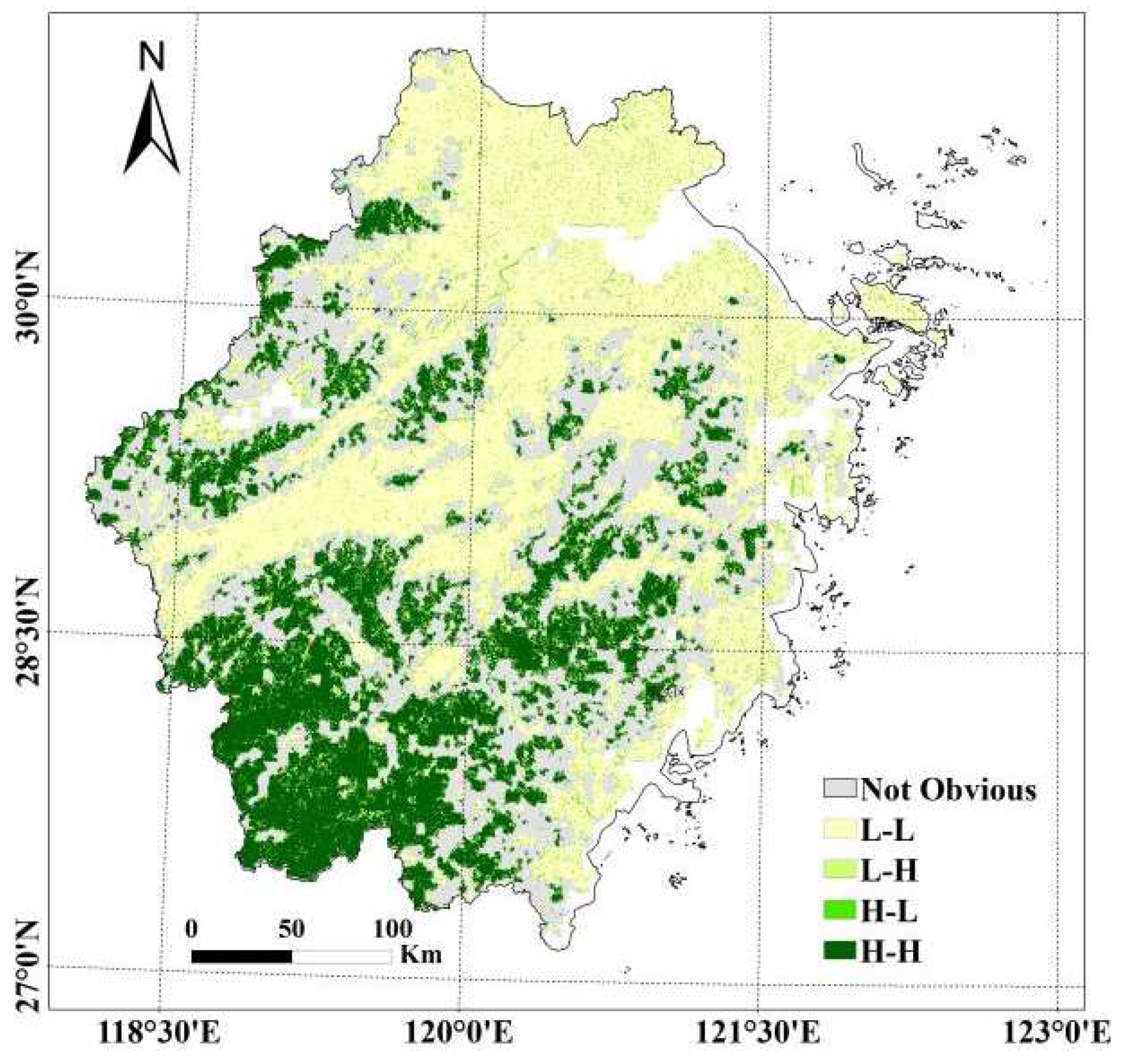
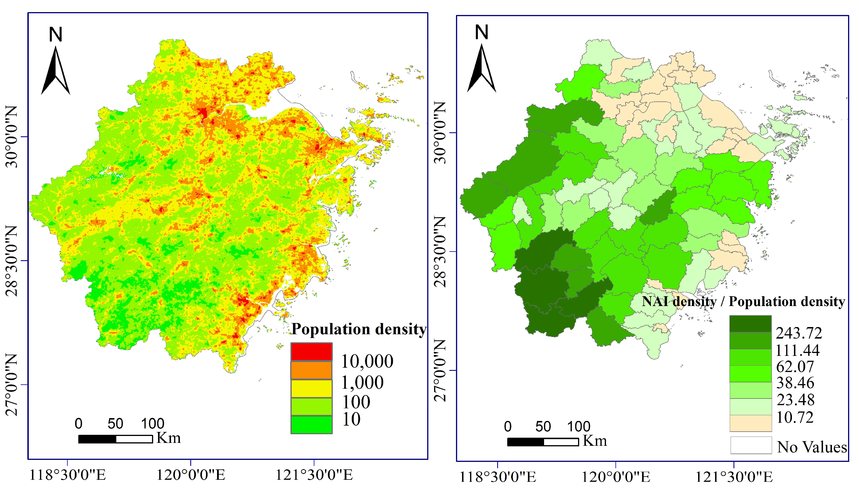
4.3. Spatio Distribution of NAIs in Zhejiang Province

With the modeling of NAI distribution, we succeeded in evaluating the spatial and temporal distribution of NAI in the Zhejiang Province of China (Figure 9). NAIs were mostly centered in the hilly southern regions where plants are most abundant, which was consistent with the terrain and SIF-determined NAI dynamics in the variable importance measures (Figure 7). The global Moran’s I of NAIs showed a strong positive spatial correlation (0.566, p < 0.005). The H–H accumulation areas of NAI concentrations were mainly distributed in woodlands. By contrast, the L–L accumulation areas were mostly observed in the middle and northern regions with vast basins and plains.

The topography was the dominant reason for these spatial patterns of NAIs. The terrain of Zhejiang Province slopes from the southwest toward the northeast [19]. Due to the vast hilly mountains, vegetation is well protected in the southern regions [36]. The luxuriant vegetation provides abundant water vapor and strong SIF flux for NAI formation [10]. Furthermore, benefiting from weak human activity [19], the passive effect of air pollution is minimized. On the contrary, vast croplands, cities, and towns are distributed in the middle basins and northern plains, where natural vegetation is severely damaged [19,36]. Meanwhile, increased impermeable ground and the urban island effect reduce the water vapor concentrations. In addition, the northern regions are close to the cities of Shanghai and Jiangsu, one of the most urbanized regions in China. Consequently, the surrounding pollutants have potentially quenched the presence of NAIs [19].

Furthermore, previous studies have conducted numerous site-based observations to reveal the NAI evolution across the whole year [9,13,15]. However, the seasonal dynamics of NAIs on a regional scale had never been achieved. In our study, based on the Fresh Air Network, we proved that the highest NAI concentration was found in summer (Figure 10), when forest productivity also peaked, revealing the regulation of plant photosynthesis on NAIs [10,20]. The lowest NAI concentration was observed in the winter. These results were consistent with previous site-based studies [10,13,37].

It is noted that the seasonal evolution pattern was consistent among different land-use types (Figure 10). Similar seasonal changes were also observed for open spaces and forests in another site-based study [13]. The coordinated variation in the driving factors across the whole year might contribute to this consistent pattern (i.e., highest in the summer and lowest in the winter) under different land types. As shown above (Figure 7), SIF, T, RH, and CO were the most important variables determining NAI variations (except topography, which was constant temporally). In the winter and autumn, cold temperatures, short photoperiods, and weak illumination intensity go against NAI formation and the rate and time of plant photosynthesis, which in turn decreases the NAIs. Meanwhile, higher air pollution in winter also has negative effects on NAI [19,38]. Meanwhile, in the summer and spring, higher temperature and humidity, stronger photosynthesis capacity, and more fresh air substantially elevate NAI concentrations [10,15]. The synchronous evolution of the driving factors co-exists in different land types.

Among the six land types, forests have the highest NAI concentrations, benefiting from the positive relationship with topography, humidity, and SIF, and the passive relationship with air pollution (Figure 8). NAI concentrations in water bodies followed forest lands. They might benefit from high water vapor and the surrounding forest lands (Figure 1), since NAIs have obvious H-H aggregation (Figure 11). It was noted that barren land had significantly higher NAI concentrations than grasslands, urban and built-up land, and cropland, while many previous studies argued that barren land usually has the lowest NAI concentrations among different land types due to the lack of vegetation [9,39]. We conceived that the higher NAI for the barren land in our study might come from the NAIs from its surroundings since it is mostly distributed in mountains with high elevation (

Table 3. The mean DEM and slope of each land type in Zhejiang Province.

OBJECTID	DEM (m)	SLOPE (°)
Barren	440.02	17.12
Built-up	54.52	3.20
Water	48.72	4.56
Grassland	344.07	16.39
Forest	413.30	18.44
Cropland	107.09	5.73

). These regions are usually surrounded by vegetation and water vapor, which favor NAI formation. As for the grasslands and cropland, lower land coverage and simple structures are not favorable for NAI formation [40,41].

In general, the fresh air resources in Zhejiang Province have reached the threshold of maintaining human health, since most regions were ranked as grade II across the whole year (Figure 8), even though the annual NAIs per capita were unevenly distributed across the entire province (Figure 11). The middle basins, northern plains, and southeast coastal regions with the highest population density had the lowest annual NAIs per capita (Figure 11). Meanwhile, NAI concentrations in most of these regions were only ranked grade III, which barely reach the margin of health maintenance. Considering the main driving factors of NAI dynamics, future work should focus on increasing urban greening and reducing pollution emissions. Meanwhile, cross-regional tourism between the northern cities and the southern mountains should be strengthened in the future.

5. Conclusions

Due to the limited NAI observation sites, regional NAIs have seldom been modeled. In this study, based on the 107 NAI stations from the Fresh Air Network, we realized the spatio-temporal modeling of NAI using an RF model when SIF was incorporated. Meanwhile, we verified the contributions of different driving factors of NAI dynamics. We also inversed the spatio-temporal distribution of NAIs in Zhejiang Province. We concluded that:

(1)

Topography dominated the spatial difference of NAIs in different regions, mostly indirectly, by controlling vegetation, climate, air quality, etc., among which the SIF was most related to the NAI dynamics;

(2)

The RF model succeeded in modeling the spatio-temporal differences in NAI among different sites, while limitations still existed;

(3)

Due to the dominance of topography, the NAI concentration in Zhejiang Province declined from the southwest to the northeast, and summer and winter have the highest and lowest NAI concentrations, respectively, for all land-use types.

Even though the mean NAI concentration in Zhejiang province reaches the threshold for maintaining basic human health, NAIs per capita were quite unevenly distributed, which dramatically increases the risk of sub-health for people living in the northern and coastal regions with the highest population density.

References

1. Villa, F.; Ceroni, M.; Bagstad, K.; Johnson, G.; Krivov, S. ARIES (ARtificial Intelligence for Ecosystem Services): A New Tool for Ecosystem Services Assessment, Planning, and Valuation. 2009. Available online: http://bioecon-network.org/pages/11th_2009/Villa.pdf (accessed on 5 November 2020).
2. Skromulis, A.; Breidaks, J.; Teirumnieks, E. Effect of Atmospheric Pollution on Air Ion Concentration. Energy Procedia 2017, 113, 231–237. [Google Scholar] [CrossRef]
3. Jiang, S.Y.; Ma, A.; Ramachandran, S. Negative Air Ions and Their Effects on Human Health and Air Quality Improvement. Int. J. Mol. Sci. 2018, 19, 2966. [Google Scholar] [CrossRef] [PubMed] [Green Version]
4. Chen, Z.; Zhang, X. Value of ecosystem services in China. Chin. Sci. Bull. 2000, 45, 870–876. [Google Scholar] [CrossRef]
5. Wen, X.; Theau, J. Assessment of ecosystem services in restoration programs in China: A systematic review. Ambio 2020, 49, 584–592. [Google Scholar] [CrossRef] [PubMed]
6. Liu, Y.; Zhou, S.; Chen, Y.; Cheng, H.; Zhou, W.; Yang, M.; Shen, Y.; Wan, L.; Su, X.; Liu, G. How do local people value ecosystem service benefits received from conservation programs? Evidence from nature reserves on the Hengduan Mountains. Glob. Ecol. Conserv. 2022, 33, e01979. [Google Scholar] [CrossRef]
7. Wang, Y.; Ni, Z.; Wu, D.; Fan, C.; Lu, J.; Xia, B. Factors influencing the concentration of negative air ions during the year in forests and urban green spaces of the Dapeng Peninsula in Shenzhen, China. J. For. Res. 2020, 31, 2537–2547. [Google Scholar] [CrossRef]
8. Nadali, A.; Arfaeinia, H.; Asadgol, Z.; Fahiminia, M. Indoor and outdoor concentration of PM10, PM2.5 and PM1 in residential building and evaluation of negative air ions (NAIs) in indoor PM removal. Environ. Pollut. Bioavailab. 2020, 32, 47–55. [Google Scholar] [CrossRef] [Green Version]
9. Wang, H.; Wang, B.; Niu, X.; Song, Q.; Li, M.; Luo, Y.; Liang, L.; Du, P.; Peng, W. Study on the change of negative air ion concentration and its influencing factors at different spatio-temporal scales. Glob. Ecol. Conserv. 2020, 23, e01008. [Google Scholar] [CrossRef]
10. Shi, G.; Yang, H.; Sang, Y.; Cai, L.; Zhang, J.; Meng, P. Relationship Between Photosynthetic Capacity and Negative Air Ion of Platycladus orientalis. Terr. Ecosyst. Conserv. 2022, 2, 13–21. [Google Scholar] [CrossRef]
11. Wang, W.; Xia, S.; Zhu, Z.; Wang, T.; Cheng, X. Spatiotemporal distribution of negative air ion and PM2.5 in urban residential areas. Indoor Built Environ. 2022, 31, 1127–1141. [Google Scholar] [CrossRef]
12. Miao, S.; Zhang, X.; Han, Y.; Sun, W.; Liu, C.; Yin, S. Random Forest Algorithm for the Relationship between Negative Air Ions and Environmental Factors in an Urban Park. Atmosphere 2018, 9, 463. [Google Scholar] [CrossRef] [Green Version]
13. Liang, H.; Chen, X.; Yin, J.; Da, L. The spatial-temporal pattern and influencing factors of negative air ions in urban forests, Shanghai, China. J. For. Res. 2014, 25, 847–856. [Google Scholar] [CrossRef]
14. Li, A.; Li, Q.; Zhou, B.; Ge, X.; Cao, Y. Temporal dynamics of negative air ion concentration and its relationship with environmental factors: Results from long-term on-site monitoring. Sci. Total Environ. 2022, 832, 155057. [Google Scholar] [CrossRef]
15. Yan, X.; Wang, H.; Hou, Z.; Wang, S.; Zhang, D.; Xu, Q.; Tokola, T. Spatial analysis of the ecological effects of negative air ions in urban vegetated areas: A case study in Maiji, China. Urban For. Urban Green. 2015, 14, 636–645. [Google Scholar] [CrossRef]
16. Guangyao, S.; Yu, Z.; Yuqiang, S.; Hui, H.; Jinsong, Z.; Ping, M.; Lulu, C. Modeling the response of negative air ions to environmental factors using multiple linear regression and random forest. Ecol. Inform. 2021, 66, 101464. [Google Scholar] [CrossRef]
17. Yue, C.; Yuxin, Z.; Nan, Z.; Dongyou, Z.; Jiangning, Y. An inversion model for estimating the negative air ion concentration using MODIS images of the Daxing’anling region. PLoS ONE 2020, 15, e0242554. [Google Scholar] [CrossRef] [PubMed]
18. Wu, C.-F.; Lai, C.-H.; Chu, H.-J.; Lin, W.-H. Evaluating and Mapping of Spatial Air Ion Quality Patterns in a Residential Garden Using a Geostatistic Method. Int. J. Environ. Res. Public Health 2011, 8, 2304–2319. [Google Scholar] [CrossRef] [PubMed]
19. Li, X.; Wu, C.; Meadows, M.E.; Zhang, Z.; Lin, X.; Zhang, Z.; Chi, Y.; Feng, M.; Li, E.; Hu, Y. Factors Underlying Spatiotemporal Variations in Atmospheric PM2.5 Concentrations in Zhejiang Province, China. Remote Sens. 2021, 13, 3011. [Google Scholar] [CrossRef]
20. Zhang, Q.; Gao, W.; Su, S.; Weng, M.; Cai, Z. Biophysical and socioeconomic determinants of tea expansion: Apportioning their relative importance for sustainable land use policy. Land Use Policy 2021, 68, 438–447. [Google Scholar] [CrossRef]
21. Chen, G.; Li, S.; Knibbs, L.D.; Hamm, N.A.S.; Cao, W.; Li, T.; Guo, J.; Ren, H.; Abramson, M.J.; Guo, Y. A machine learning method to estimate PM2.5 concentrations across China with remote sensing, meteorological and land use information. Sci. Total Environ. 2018, 636, 52–60. [Google Scholar] [CrossRef] [PubMed]
22. Mosavi, A.; Rabczuk, T.; Varkonyi-Koczy, A.R. Reviewing the Novel Machine Learning Tools for Materials Design; Recent Advances in Technology Research and Education; Springer: Berlin, Germany, 2017. [Google Scholar]
23. Wu, C.C.; Lee, G.W.; Yang, S.; Yu, K.P.; Lou, C.L. Influence of air humidity and the distance from the source on negative air ion concentration in indoor air. Sci. Total Environ. 2006, 370, 245–253. [Google Scholar] [CrossRef] [PubMed]
24. Shi, G.; Huang, H.; Sang, Y.; Cai, L.; Zhang, J.; Cheng, X.; Meng, P.; Sun, S.; Li, J.; Qiao, Y. Solar-induced chlorophyll fluorescence intensity has a significant correlation with negative air ion release in forest canopy. Atmos. Environ. 2021, 269, 118873. [Google Scholar] [CrossRef]
25. Wang, M.; Wang, H. Spatial Distribution Patterns and Influencing Factors of PM2.5 Pollution in the Yangtze River Delta: Empirical Analysis Based on a GWR Model. Asia-Pac. J. Atmos. Sci. 2021, 57, 63–75. [Google Scholar] [CrossRef]
26. Deng, L.; Deng, Q. The basic roles of indoor plants in human health and comfort. Environ. Sci. Pollut. Res. 2018, 25, 36087–36101. [Google Scholar] [CrossRef]
27. Breiman, L. Random Forests. Mach. Learn. 2001, 45, 5–32. [Google Scholar] [CrossRef] [Green Version]
28. Deng, X.; Long, R.; Gao, C.; Xiong, Y. Metal-organic frameworks for artificial photosynthesis via photoelectrochemical route. Curr. Opinion Electrochem. 2019, 17, 114–120. [Google Scholar] [CrossRef]
29. Skalny, J.D.; Mikoviny, T.; Vladoiu, R. Negative corona discharges in pure CO2 and/or N2O gases and their mixtures with oxygen. Rom. J. Phys. 2004, 49, 321–331. [Google Scholar]
30. Sinicina, N.; Skromulis, A.; Martinovs, A. Impact of Microclimate and Indoor Plants on Air Ion Concentration. In Proceedings of the International Scientific and Practical Conference, Environment Technology Resources, St. Petersburg, Russia, 6–8 October 2015. [Google Scholar]
31. Chen, Q.; Wang, R.; Zhang, X.; Liu, J.; Wang, D. Effects of Different Site Conditions on the Concentration of Negative Air Ions in Mountain Forest Based on an Orthogonal Experimental Study. Sustainability 2021, 13, 2012. [Google Scholar] [CrossRef]
32. Lou, W.; Yao, Y.; Sun, K.; Deng, S.; Yang, M. Variability of heat waves and recurrence probability of the severe 2003 and 2013 heat waves in Zhejiang Province, southeast China. Clim. Res. 2019, 79, 63–75. [Google Scholar] [CrossRef]
33. Tomo’omi, K.; Kuraji, K.; Noguchi, H.; Tanaka, Y.; Suzuki, K.T.M. Vertical profiles of environmental factors within tropical rainforest, Lambir Hills National Park, Sarawak, Malaysia. J. For. Res. 2001, 6, 257–264. [Google Scholar] [CrossRef]
34. Regaieg, O.; Yin, T.; Malenovsky, Z.; Cook, B.D.; Morton, D.C.; Gastellu-Etchegorry, J.-P. Assessing impacts of canopy 3D structure on chlorophyll fluorescence radiance and radiative budget of deciduous forest stands using DART. Remote Sens. Environ. 2021, 265, 112673. [Google Scholar] [CrossRef]
35. Huang, K.; Xiao, Q.; Meng, X.; Geng, G.; Wang, Y.; Lyapustin, A.; Gu, D.; Liu, Y. Predicting monthly high-resolution PM2.5 concentrations with random forest model in the North China Plain. Environ. Pollut. 2018, 242, 675–683. [Google Scholar] [CrossRef] [PubMed]
36. Li-wang, S.; Jian, D.; Wei-min, W.; De-hui, Q. Temporal and Spatial Variations of Vegetation Coverage in Zhejiang Province Based on MODIS Data. J. Yangtze River Sci. Res. Inst. 2021, 38, 40–46. [Google Scholar] [CrossRef]
37. Cao, J.; Zhang, B.; Zhang, Y.J.E.; Sciences, E. Characteristics of Air Anion Distribution in Beach and Forest Environment and the Correlation between Air Anion and the Environmental Factors. Ecol. Environ. Sci. 2017, 26, 1375–1383. [Google Scholar] [CrossRef]
38. Retalis, A.; Nastos, P.; Retalis, D. Study of small ions concentration in the air above Athens, Greece. Atmos. Res. 2009, 91, 219–228. [Google Scholar] [CrossRef]
39. Chen, A.; Mao, J.; Ricciuto, D.; Xiao, J.; Frankenberg, C.; Li, X.; Thornton, P.E.; Gu, L.; Knapp, A.K. Moisture availability mediates the relationship between terrestrial gross primary production and solar-induced chlorophyll fluorescence: Insights from global-scale variations. Glob. Change Biol. 2021, 27, 1144–1156. [Google Scholar] [CrossRef]
40. Bai, B.; Chen, D.; Xu, T.; Shen, Z.; Cao, H.J.E.a.; Sciences, E. Differences in the Changes of Negative Air Ion Concentration among Different Vegetation Types in North Central Henan Province, China. Ecol. Environ. Sci. 2016, 25, 1629–1637. [Google Scholar] [CrossRef]
41. Xing, H.; Tang, Q.; Dongyou, Z. Air Anion Concentration: Difference in Different Underlying Surfaces in Mohe. Chin. Agric. Sci. Bull. 2017, 33, 101–105. [Google Scholar]
Figure 1. The distribution of 107 stable monitored NAI sites and the land-use types across Zhejiang province.
Remotesensing 15 00738 g001
Figure 2. Flowchart of NAI estimation based on RF algorithm.
Remotesensing 15 00738 g002
Figure 3. Relationship between Ntrees and OOB.Error.
Remotesensing 15 00738 g003
Figure 4. R2 (a) and RMSE (b) for different combinations of Minleaf and Mtry.
Remotesensing 15 00738 g004
Figure 5. Model training results (left) and verification results (right) of the RF algorithm.
Remotesensing 15 00738 g005
Figure 6. Importance of each feature in the model.
Remotesensing 15 00738 g006
Figure 7. Path analysis diagram illustrating relationships among terrain (DEM, aspect, slope), environmental factors (T, CO, RH), plant photosynthesis (SIF), and NAIs and the total effects of the drivers on NAIs for all land types (a1,a2), forest land (b1,b2), urban and built-up lands (c1,c2), and cropland (d1,d2).
Remotesensing 15 00738 g007
Figure 8. Estimated results of NAI concentrations in Zhejiang Province from January to December 2020. Roman numerals refered to the NAI grades, I: NAI > 2000 ions cm−3; II: 1000 < NAI ≤ 2000 ions cm−3; III: 500 < NAI ≤1000 ions cm−3; IV: NAI ≤ 500 ions cm−3.
Remotesensing 15 00738 g008
Figure 9. LISA aggregation map of NAI concentrations in Zhejiang in 2020.
Remotesensing 15 00738 g009
Figure 10. Intra-annual variation in NAI concentrations for different land-cover types. Different letters referred to the significant difference among the land types (p < 0.05).
Remotesensing 15 00738 g010
Figure 11. The population density and the ratio of annual mean NAI concentrations to population density in the different counties of Zhejiang province.
Remotesensing 15 00738 g011