Article

Insights into the Effect of Urban Morphology and Land Cover on Land Surface and Air Temperatures in the Metropolitan City of Milan (Italy) Using Satellite Imagery and In Situ Measurements

by
Mathilde Puche
,
Alberto Vavassori
and
Maria Antonia Brovelli
*
Department of Civil and Environmental Engineering, Politecnico di Milano, Piazza Leonardo da Vinci 32, 20133 Milano, Italy
*
Author to whom correspondence should be addressed.
Remote Sens. 2023, 15(3), 733; https://doi.org/10.3390/rs15030733
Submission received: 15 November 2022 / Revised: 23 January 2023 / Accepted: 25 January 2023 / Published: 27 January 2023

Abstract

:
With a concentration of people, activities, and infrastructures, urban areas are particularly vulnerable to the negative effects of climate change. Among others, the intensification of the Urban Heat Island (UHI) effect is leading to an increased impact on citizen health and the urban ecosystem. In this context, this study aims to investigate the effect of urban morphology and land cover composition—which are established by exploiting the Local Climate Zone (LCZ) classification system—on two urban climate indicators, i.e., Land Surface Temperature (LST) and air temperature. The study area is the Metropolitan City of Milan (northern Italy). LCZ and LST maps are derived by leveraging satellite imagery and building height datasets. Both authoritative and crowdsourced in situ measurements are used for the analysis of air temperature. Several experiments are run to investigate the mutual relation between LCZ, LST, and air temperature by measuring LST and air temperature patterns in different LCZs and periods. Besides a strong temporal correlation between LST and air temperature, results point out vegetation and natural areas as major mitigating factors of both variables. On the other hand, higher buildings turn out to increase local air temperature while buffering LST values. A way lower influence of building density is measured, with compact building areas experiencing slightly higher air temperature yet no significant differences in terms of LST. These outcomes provide valuable tools to urban planners and stakeholders for implementing evidence-based UHI mitigation strategies.

1. Introduction

Urban areas currently host more than 55% of the world’s population [1] and 75% of the European citizens [2]. Accounting for more than 70% of the global carbon dioxide emissions [3], cities are considered major contributors to climate change while being at the same time among the most vulnerable targets of its negative effects [4]. With a concentration of people, activities, and infrastructures, cities will be increasingly affected by water shortages, risk of flooding, and citizen health problems connected with heat waves and reduced air quality, among others [5].
In particular, the increasing frequency and intensity of heat waves [6] along with the gradual substitution of natural and vegetated areas with artificial surfaces is leading to the intensification of the Urban Heat Island (UHI) effect [7,8]. UHIs are identified where the temperature patterns are significantly warmer in urban areas than in the surrounding rural environment. Several factors contribute to the UHI, including the ability of urban surfaces to absorb and store heat, urban greenness loss, anthropogenic heat fluxes, and the urban canyon effect [9]. Given the direct impact of UHIs on human health, energy consumption, and urban ecosystems [10,11,12], several studies have been carried out to investigate the causes and consequences of UHIs [13]. However, many research works are focused on the analysis of temperature differences between the urban area and the neighboring rural environment. This approach oversimplifies the investigation of the urban climate, which is typically characterized by local-scale temperature differences and space-time patterns.
To address the inadequacy of the urban–rural dichotomy for the analysis of UHI in urban agglomerates, a climate-based classification system called Local Climate Zone (LCZ) was developed [14]. This classification defines 17 unique area types based on the physical and thermal properties of their surface. For this reason, it is widely employed to account for urban morphology and land cover in urban climatology studies [15,16]. LCZ maps are generally computed by leveraging EO satellite imagery in conjunction with multiple ancillary geo-data. According to the World Urban Database and Access Portal Tools (WUDAPT) project protocol [17,18], LCZ maps may be derived from the supervised classification of optical satellite imagery. This approach demands the collection of independent training and testing samples, which may be constructed exploiting suitable datasets including land cover and land consumption layers as well as local topographic databases.
Starting from the LCZ classification, the influence of urban morphology and land cover on the UHI may be investigated by considering two climate-related variables—namely Land Surface Temperature (LST) and air temperature. Despite being certainly correlated measures [19], the two variables have different physical meanings. The former is strictly related to the energy flux emitted by the surface, whereas the latter is an indicator of the local atmospheric conditions [20]. Since the two variables provide complementary information, a thorough investigation of the UHI effect should comprise the analysis of both land surface and air temperature [21]. However, most of the studies available in the literature focused on the analysis of only one of the two variables. For instance, the relationship between LCZ and LST was investigated in [22,23] using satellite imagery to compute the LST distribution. The authors found that LST values are significantly higher in built-up areas than across natural surfaces. Furthermore, heavy industry, dense low-rise building, and compact mid-rise building areas were found to experience the highest LST, while water and densely forested areas exhibited cooler temperature values. On the other hand, the relation between LCZ and air temperature was studied in [24], where they found that night-time temperatures are, on average, 4 °C higher in impervious and built-up areas than in vegetated zones. The influence of vegetation on the urban climate is directly related to the evapotranspiration-cooling and leaf area index-shading effects [25]. In [26,27], the air temperature distribution was measured through mobile surveys. The former study revealed that temperature amplitude is lower during night-time in urbanized LCZ types, with average variations ranging from 0.2 °C to 4.4 °C in the different LCZ types. The latter pointed out that the maximum temperature values are experienced in compact mid-rise areas, whereas cooler temperatures are recorded in open-set and sparsely built regions.
The combined analysis of LST and air temperature is complicated by the different technologies which are required for their measurement. Specifically, while the surface temperature can be easily acquired by satellite sensors, air temperature is measured by ground-based sensors. In situ sensors usually belong to official weather stations that rely on regional infrastructure for the collection of meteorological data. Despite acquiring data with high accuracy and temporal frequency, official stations provide few point samples whose distribution is rarely designed to effectively reflect spatial variations in air temperature [28]. In contrast, official weather stations are set up for climate monitoring and weather forecasting purposes and are therefore generally installed outside the urban centers to limit the temperature bias connected with the UHI effect [29].
For these reasons, some approaches have been developed aiming to derive an estimate of the near-surface air temperature from remotely sensed LST maps. The use of LST as a proxy of air temperature would compensate for the limited spatial coverage of on-ground measurement networks and provide information where local sensors are not available. However, general and straightforward procedures are hard to achieve, since the correlation between LST and air temperature is quite dependent on local weather conditions and surface characteristics and variable between day-time and night-time [30,31]. An alternative solution to improve the granularity of on-ground measurements consists in turning to non-traditional data sources such as low-cost citizen weather stations. These stations are brought by individuals to collect meteorological parameter measurements which are distributed by commercial or non-profit organizations. Observations are in most cases voluntarily collected by amateurs with a similar motivation to contribute to local climate monitoring [32]. Literature has seen many authors developing approaches that take advantage of crowdsourced data for mapping air temperature at the urban level [33,34]. Despite the undeniable advantages, the accuracy of crowdsourced data is questionable since no quality check is performed. Among the multiple sources of errors affecting crowdsourced weather observations, it is worthwhile mentioning the poor quality or the lack of calibration of the monitoring instruments, as well as the inconvenient device siting (e.g., close to the building’s wall, or underneath vegetation), which may lead to systematic errors in the time series [34]. Accordingly, the use of citizen-generated data demands data cleaning and pre-processing aiming to remove local and global outliers [35].
Based on the literature summarized above, a gap appears in the research for common mitigating factors of both LST and air temperature in the urban environment. For this reason, the present study aims to investigate the relationship between LCZs, LST, and air temperature to quantify the effect of urban morphology and land cover on both climate-related indicators. This goal is accomplished by leveraging multiple geo-data, including high-resolution Landsat 8 satellite imagery as well as authoritative and crowdsourced air temperature observations. The Metropolitan City of Milan (northern Italy) was selected as a case study. A preliminary analysis of the influence of urban land cover on air temperature with geo-data and satellite imagery for the city of Milan was presented in [36]. However, the present work aims to go deeper into the investigation of urban climate by considering a wider study area, a longer period, and focusing on the analysis of both LST and air temperature.
The remainder of this paper is structured as follows. Section 2 describes the study area, the data sources, and the software technology used. Section 3 introduces the methodology employed to compute the LCZ and LST maps and process the air temperature observations. Section 4 presents and discusses the results, pointing out the relationship between LCZ, LST, and air temperature. Finally, in Section 5, a discussion of the obtained results is reported, and the main conclusions are presented.

2. Materials

2.1. Study Area and Time Range

The analysis carried out in this study is focused on the Metropolitan City of Milan, which is located in the Lombardy Region, northern Italy (see Figure 1). The area covers 1575 km2 and includes the city of Milan and other 133 municipalities. With more than 3 million inhabitants [37], it is the second most populous Metropolitan City in Italy after Rome. The area is entirely flat, with an altitude ranging from 98 to 199 m above sea level. According to the Köppen–Geiger Climate Classification [38], its climate can be summarized as warm temperate, fully humid with hot summer, as most of the inland plain cities in northern Italy. According to the official measurements of the Milano Linate historical weather station [39] the average monthly temperature fluctuates between 2.5 °C (January) and 23.6 °C (July); however, temperature peaks higher than 35 °C are becoming increasingly frequent during summer, with a record temperature of 39.3 °C measured in August 2003. In addition, Milan suffers from poor wind circulation, which causes stagnation of fog and pollutants [40] and favors the persistence of the UHI effect [41]. This makes this area a suitable target for the investigation of local climate effects.
The Metropolitan City was selected rather than the city of Milan to comprise a wider range of climate zones in the analysis. Since urbanization is mainly concentrated in Milan, which hosts almost 40% of the whole area’s population, the surrounding urban centers as well as rural and natural areas were included to best appreciate the UHI effect and local climate differences.
A preliminary investigation of the evolution over time of land consumption, in terms of artificialization, in the study area was conducted to define the most suitable time range for LCZ mapping. The analysis of data distributed by the Italian Institute for the Environmental Protection and Research (ISPRA) [42] pointed out that very small changes in terms of land consumption occurred since 2006. The most appreciable change is represented by a motorway (A58) which was constructed in the eastern portion of the Metropolitan City in June 2012. However, such variations of land consumption cannot be properly accounted into a LCZ segmentation, since LCZ maps are meant to delineate uniform climate regions extending over hundreds of meters to kilometers [14]. Accordingly, the year 2021 was selected for the analysis to best represent the most recent conditions in terms of land cover and use.
The analysis of land surface and air temperatures was carried out by focusing on the most recent years, namely from 2018 to 2022, which provide sufficiently numerous data samples.

2.2. Data Collection

Data collected for the analysis mainly consist of optical satellite imagery, ancillary geospatial datasets, and in situ air temperature measurements. Data used in this work are entirely released under fully open licenses or custom open licenses allowing for its exploitation for research purposes.

2.2.1. Satellite Imagery

Multispectral satellite imagery was exploited for both LCZ and LST mapping. Among the numerous missions, Landsat 8 was chosen in this study for several reasons. Firstly, it provides global coverage and freely available imagery which enables the replicability and improvement of the proposed approach. Moreover, it acquires images in 11 different spectral bands through an optical sensor (the Operational Land Imager, OLI) and a thermal sensor (the Thermal Infrared Sensor, TIRS), providing the potential to generate both LCZ and LST maps from a single acquisition. Furthermore, the spatial resolution of the optical sensor (i.e., 30 m) may be considered a good trade-off for LCZ mapping purposes [18]. The Collection 2 Level 2 (C2L2) product of the Landsat 8 mission was exploited since it provides analysis-ready Bottom-of-Atmosphere (BOA) reflectance data as well as geophysical parameters such as surface temperature values.
Five images related to the year 2021 were exploited for LCZ mapping. The motivation behind the use of multiple imageries for a single final LCZ classification is twofold. The first reason is to account for seasonal variations in land cover composition (i.e., vegetative and non-vegetative periods). The second reason is to increase classification accuracy, as found in [18]. Optical bands from 1 to 7 (with 30 m spatial resolution) were used, which correspond to the aerosol, visible, near infrared (NIR), and short-wave infrared (SWIR) wavelengths of the electromagnetic spectrum.
Four cloud-free images from 2020 to 2022 were selected for mapping LST as well as analyzing the relation between LST and LCZ. The selection was limited to images with very limited cloud cover (i.e., <5%) acquired during summer to detect the highest annual temperatures experienced across the study area. The computation of the LST maps relied entirely on the use of the thermal infrared (TIR) band. Despite two thermal bands being available, namely Band 10 and Band 11, only the former was used as widely suggested in the literature owing to the calibration errors of Band 11 [43]. Band 10 was originally provided at 100 m spatial resolution, however, data were downscaled and distributed by the provider with a resolution of 30 m.
The Landsat 8 images used for LCZ and LST mapping are summarized in Table 1, where the date of acquisition of each image is reported. The number of images used for the correlation test between LST and air temperature was increased to guarantee the statistical validity of the analysis. Accordingly, a total number of 36 acquisitions from 2018 to 2021 were leveraged for this purpose. Images were selected to be uniformly distributed throughout the year as well as meet the limited cloud cover requirements of the analysis. For the sake of conciseness, the list of images is not reported.

2.2.2. Ancillary Datasets

Ancillary open geo-data provided by multiple sources were exploited for defining training and testing areas. Specifically, the land consumption dataset distributed by ISPRA [42], which provides a segmentation of the Italian national territory in 12 land use classes with 10 m resolution, the building height dataset provided by the Lombardy Region within the regional topographic database [44], and very high resolution (i.e., ~15 cm) Google Satellite imagery which was retrieved through the plugin [45] in QGIS were used.

2.2.3. Air Temperature Observations

For the air temperature analysis, official weather observations collected and distributed by the Regional Agency for Environmental Protection (ARPA) were exploited. Data were recorded with a temporal frequency of 10 min by 15 stations distributed across the Metropolitan City of Milan. Time series length depended on the installation date of each station, with the oldest station recording temperature measurements since 1989. Data were downloaded through the Open Data Portal of the Lombardy Region [46] in comma-separated values (CSV) format.
Additional weather stations were considered in this study to increase the spatial coverage of on-ground temperature observations. Crowdsourced measurements were collected from the Netatmo amateur network [47]. Netatmo is a commercial manufacturer and data aggregator of citizen weather stations, distributing low-cost weather stations for citizens around the world with the aim of monitoring outdoor and indoor weather conditions (e.g., temperature and humidity). Netatmo stations take advantage of Wi-Fi connection for data transfer and automatic upload on a dedicated server, and owners have access to real-time data visualization via application software. Observations are publicly shared through a dedicated Application Programming Interface (API), which enables free data download within the limits expressed by the provider.
In this study, Netatmo data were retrieved through a custom Python code that was developed by the authors. The code takes advantage of the Python package patatmo [48] and specifically of two dedicated methods. The former is used to get instantaneous measurements from all stations within a specific geographic area along with the corresponding metadata (e.g., station identifier, latitude, and longitude). The latter allows data retrieval for a specific station in a given time range and is thus used to extract temperature time histories recorded by each station.
The collected temperature time series from both ARPA and Netatmo stations refer to the period 2018–2021, which was here considered for the air temperature analysis. The number of Netatmo stations increases over time, ranging from 368 in 2018 to 688 in 2021. The distribution of ARPA and Netatmo stations for the year 2021 is depicted in Figure 2. This representation clearly shows that Netatmo stations are mainly concentrated in urbanized areas rather than in rural zones, since the devices are typically installed at the amateur’s place of residence.

2.3. Software Tools and Programming Languages

Free and Open Source Software (FOSS) was solely used in this work for data processing, analysis, and mapping. QGIS was primarily used for geodata management and visualization, including vector data digitizing and processing and multiband raster creation. The System for Automated Geoscientific Analyses (SAGA) was largely exploited to perform classification post-processing. The programming languages Python and R were used for code development. In particular, Python was used for Netatmo data extraction and cleaning and the computation of statistics and graphs (e.g., boxplots). Popular libraries were used for this purpose, such as pandas [49] and fiona [50]. The dedicated library patatmo was used for Netatmo data extraction. On the other hand, the R packages raster [51] and randomForest [52] were exploited for the application of the supervised classification algorithm on satellite imagery.

3. Methods

3.1. Local Climate Zones (LCZ) Mapping

The LCZ concept comprises 17 classes, divided into 10 artificial and 7 natural classes, which depend on the physical and thermal properties of the surface. More specifically, the definition of each LCZ is primarily related to the urban morphology (in terms of height and density of buildings and trees) and the land cover composition (in terms of surface perviousness). In the Metropolitan City of Milan, only 8 classes were found out of the 17 classes originally defined in [14]. A detailed description of each class is presented in Table 2.
To derive the LCZ map of the Metropolitan City of Milan from Landsat 8 images, the workflow summarized in Figure 3 was followed. To take into account the seasonal evolution of vegetation in the final LCZ map, one Landsat 8 scene per season for the year 2021 was exploited, resulting in a total number of four images; a further image was then employed to improve the result. By adding a post-processing step to the resulting LCZ maps, the methodology followed in this work extends the protocol established by the WUDAPT project [18]. Such protocol includes the creation of a training dataset and the application of a supervised classification algorithm—which is typically the Random Forest (RF) —on multispectral satellite imagery to achieve a segmentation of the area of interest into LCZs. A detailed description of each step is provided in the following subsections.

3.1.1. Construction of Train and Test Datasets

The classification performed in this protocol takes advantage of a supervised classification algorithm that requires a labeled dataset, called training dataset, to learn to associate new unclassified data (pixels) to the defined set of classes. Starting from the work presented in [53], where the author created a training dataset for the City of Milan, training areas were here extended to the entire Metropolitan City and completed with missing classes. To do so, a combined analysis of the building height dataset and very high-resolution Google Satellite imagery was performed. The training data were also equally distributed among the eight classes to guarantee an even representation of each LCZ type and thus improve classification accuracy. In addition, to avoid any correlation between training and testing data, the aforementioned procedure was repeated to produce an independent, so-called “out-of-bag”, testing dataset.

3.1.2. Random Forest (RF) Classification

The supervised, pixel-based classification algorithm adopted in this work for LCZ mapping is the RF, which offers a good compromise between achieved accuracy and computational performance [18]. The RF algorithm creates several decision trees on data samples, gets the prediction from each of them, and finally selects the best solution through majority voting. Among the numerous advantages, the algorithm is non-parametric and requires limited data pre-processing while providing high accuracy and fast computational performance. Moreover, the RF algorithm contains an internal validation, with 2/3 of the training dataset used for learning and the remaining 1/3 for testing the model accuracy. This is particularly helpful when creating the training areas since the internal validation of the algorithm can be leveraged to get a first estimate of the overall accuracy of the result. Accordingly, the training dataset was here iteratively updated until a satisfactory global accuracy was obtained.
To carry out the RF classification, the algorithm implemented in RStudio in [54] was exploited. For each of the four pre-processed Landsat 8 images, the classification was run, resulting in four LCZ maps.

3.1.3. Post-Processing and Accuracy Assessment

Pixel-based classification algorithms such as the RF typically produce a “salt-and-pepper” noise in the output. This effect is often removed through a post-processing step to achieve a smoother classification map. For this reason, a majority filter with 2 × 2 (pixels) moving window was applied to each of the obtained LCZ maps using SAGA. The filtered images were then combined through majority voting, resulting in the final LCZ map.
To assess the accuracy of the result, the confusion matrix was computed using the Semi-Automatic Classification Plugin (SCP) in QGIS and the independent testing set. Common accuracy measures were derived from the confusion matrix, including: (i) Overall Accuracy (OA): percentage of correctly classified pixels with respect to the total number of pixels; (ii) Producer’s Accuracy (PA): percentage of pixels correctly classified in each class with respect to the number of pixels belonging to that class; and (iii) User’s Accuracy (UA): percentage of pixels correctly classified in each class with respect to the number of pixels predicted to belong to that class. The OA is a general evaluation of the model, whereas PA and UA provide a class-by-class assessment of its performance.

3.1.4. Classification Improvement

Two main shortcomings can be highlighted in the procedure outlined above. Firstly, the application of majority voting to the seasonal LCZ maps outputs a “no-data” value whenever no majority is found, while it is preferable to limit the number of unclassified pixels in the final map. Secondly, some built-up types (namely, classes 3, 5, 6, and 8) show poor spectral separability at the Landsat 8 bands’ wavelengths, which prevents the classifier from properly differentiating these artificial classes. Additional data was therefore used to overcome these limitations and improve the classification output.
Specifically, since the number of unclassified pixels is generally higher when merging an even number of maps, a further satellite image (i.e., the 16 March 2021 image) was added to the classification workflow, so that five LCZ maps are produced. Furthermore, the building height vector layer was converted to a 30 m resolution raster and merged into each of the five Landsat 8 images as an additional feature band. Indeed, the study presented in [55] proves that incorporating the building height layer as a new band to the input multispectral image may significantly improve the detection and distinction of built-up classes.
The RF classification was run on each of the five eight-band raster images, and the same post-processing and accuracy assessment presented in the previous sub-Section were finally carried out.

3.2. Land Surface Temperature (LST) Analysis

The steps followed to retrieve the LST from Landsat 8 C2L2 product and analyze its variation in the different LCZs are summarized in Figure 4.
Specifically, the LST distribution in the study area was computed and mapped using four Landsat 8 images relative to the summers 2021 and 2022. Being the Landsat 8 C2L2 product analysis-ready, the LST values could be directly computed from Band 10 by simply applying a linear transformation to the digital numbers ( D N s), as shown in Equation (1):
L S T K e l v i n = 0.00341802   D N + 149  
The LST was computed in Kelvin and then transformed into Celsius degrees by subtracting 273.15 to each pixel value. Cloud-contaminated pixels were identified and subtracted from the LST map using the CloudMasking plugin in QGIS [56], since cloud apparent temperatures are typically much lower than the actual surface temperature, as shown in [57].
Once the four LST maps were retrieved, the LCZ map of the Metropolitan City of Milan was exploited to compute the temperature statistics per class. Two separate analyses were carried out focusing on (i) the temperature difference between artificial and natural classes and (ii) the temperature difference between the various built-up classes.
The first test was performed by merging the eight LCZ classes into two groups, namely “artificial” and “natural” areas. The LST mean and standard deviation for the two categories were computed and the statistical and practical significance of LST difference between artificial and natural areas was further explored by leveraging the two-sample z-test and computing the Cohen’s d and the Confidence Intervals (CIs), as explained in the following.
Given the large sample size (i.e., >175,000 pixels), the normal distribution for the LST was assumed, allowing for the computation of the z-score as well as the corresponding p-value. Accordingly, the statistical significance of the LST difference between artificial and natural classes was verified. However, when dealing with large samples, the p-value quickly falls to zero, leading to rejecting the null hypothesis of equal means between the two samples without considering the “practical” significance of the result [58]. For these reasons, the effect size—which is a measure of the effective size of the means’ difference—was checked by computing the Cohen’s d. The interpretation of the size effect, from negligible to huge, followed the thresholds defined by Cohen in [59]. As a complement, the CIs at 95% confidence level were calculated to assess the variation around the estimated LST difference.
A similar analysis was performed focusing on artificial surfaces (i.e., classes 2, 3, 5, 6, and 8). Specifically, the LST mean and standard deviation for each built-up type were computed. The same statistics described above were calculated for each pair of artificial classes to investigate the statistical and practical significance of the surface temperature differences within the built-up types. In this case, the one-way ANOVA (analysis of variance) test was also carried out for comparing the temperature means of the five groups.

3.3. Air Temperature Analysis

The second climate-related variable considered in this study is air temperature, which is the most commonly ground-based measured meteorological parameter given its relevance in climate and global change research. Air temperature analysis was carried out considering the period 2018–2021. As a first step, in situ measurements from both ARPA and Netatmo stations were cleaned and pre-processed through Python scripting. Then, the correlation between air temperature and LST was investigated as well as air temperature variations between different LCZs and periods.

3.3.1. Time Series Cleaning

Since crowdsourced temperature time series were largely exploited for the analysis, a preliminary data-cleaning step was carried out. Indeed, these observations are subject to two main types of uncertainties, namely measurement uncertainties, due to the unknown accuracy of the station measurement, and contextual uncertainties, related to the unknown exact sensor position [33]. Official ARPA station measurements were used as a reference for cleaning Netatmo time series. However, the downloaded ARPA data required three steps pre-processing that was implemented for all years from 2018 to 2021 (see Figure 5).
Specifically, from the original raw data containing the measurements from all the weather stations in the Lombardy Region, only temperature measurements recorded by the 15 stations of the Metropolitan City of Milan were retained. Despite meeting the quality standards required by the Italian national legislation, outlier measurements in the time series were detected and removed using the z-score method. Finally, the time series of a virtual ARPA station was computed as the hourly average of the measurements recorded by the 15 ARPA stations. The virtual ARPA station was considered as a reference for the following Netatmo data cleaning.
Different types of outliers were detected and removed from the Netatmo time series, as depicted in Figure 5. While uncorrelated times series with respect to the virtual ARPA station were identified with a Pearson’s coefficient lower than 0.6, unrealistic observations were removed using the monthly minimum and maximum temperatures of the reference time series. The biased times series, having a globally higher or lower mean than the reference, were excluded using the hourly values of the virtual station. Finally, a 3-h window moving average was applied to each time series to single out potential local outliers. This four-step processing was applied to the data from 2018 to 2021 and resulted in the final cleaned Netatmo dataset, which was used for the following analyses.

3.3.2. Correlation between Air Temperature and LST

The relationship between LST and air temperature has been extensively studied in recent years [28,31,60]. The growing interest in understanding the correlation between these climate-related variables is primarily connected with the possibility to derive space-resolved air temperature estimates from remotely sensed LST measurements. This would overcome the intrinsic limitations in the detection of air temperature from in situ sensors with very high spatial resolution, which is demanded for micro-climate studies. The temporal correlation between LST and air temperature is typically assessed by considering the time series of the two variables in specific point locations over a defined time period and computing common correlation coefficients [30,61,62]. On the other hand, the spatial correlation is evaluated by comparing the spatial distribution of the two variables at a specific time instant and computing similar correlation measures.
For the purposes of the present study, both the temporal and spatial correlation between LST and air temperature were investigated. For a consistent comparison of the two variables, the average air temperature recorded at each station location between 9:00 a.m. and 11:00 a.m. (GMT) were computed, since LST is measured by the satellite sensor at 10:10 a.m. (GMT) in the area of interest for the selected dates. More specifically, the temporal correlation was assessed considering 36 dates corresponding to all Landsat 8 scenes with less than 5% cloud coverage in the time interval 2018–2021. In turn, the spatial correlation was computed considering the LST maps derived for summer 2021, namely 6th and 22 July 2021. The Pearson’s coefficient was calculated for the evaluation of both temporal and spatial correlation.

3.3.3. Analysis of Air Temperature per LCZ

The LCZ map was also exploited to compute the air temperature statistics per class over the period 2018–2021. Air temperature patterns were investigated considering (i) the whole study period as well as (ii) different seasons, to explore possible variations of air temperature per LCZ in various time intervals. The steps followed for this analysis are summarized in Figure 6. Each temperature station location was associated with the corresponding LCZ class. For the first test (i), the yearly average temperature recorded at each station was calculated and the statistics per LCZ class were easily derived. Similar to the LST analysis, the statistical and practical significance of the air temperature means’ difference per class were assessed through ANOVA and paired t-tests as well as the computation of the Cohen’s d. While the z-test was used for the LST, the t-test was preferred in this case since the assumptions (i.e., sample independence, normality, and homogeneity of variance) are met by the air temperature distribution per LCZ. For the second experiment (ii), the same workflow was followed considering the seasonal average of air temperature at each station location.

4. Results

4.1. LCZ Map

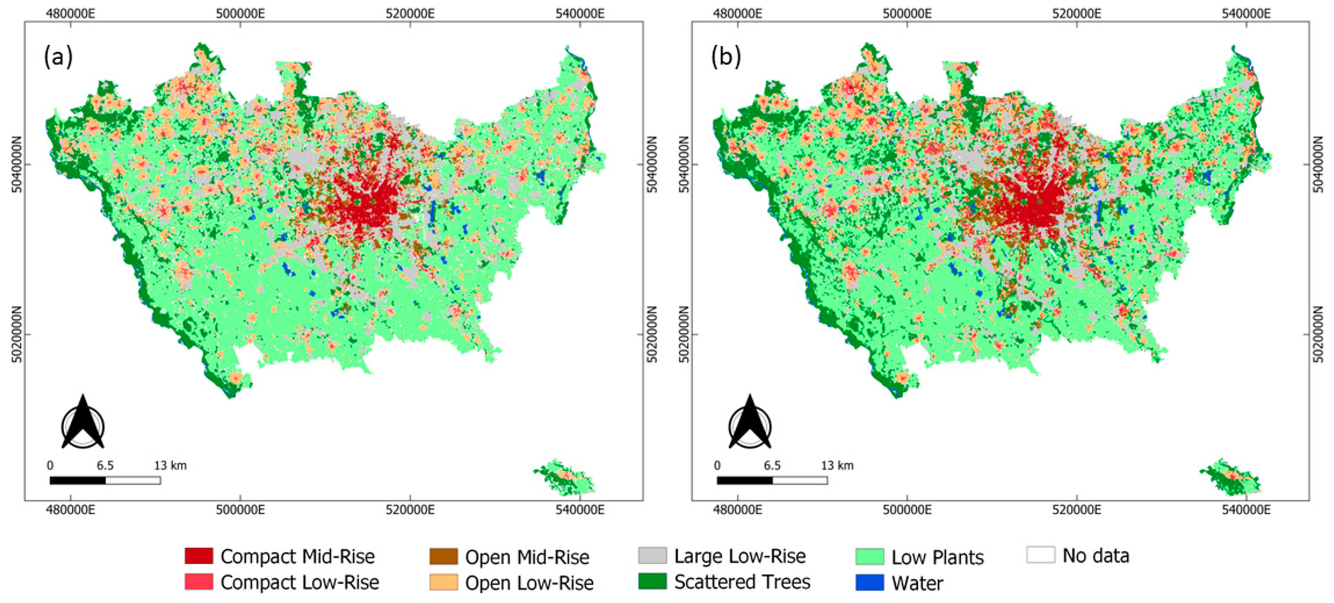
The obtained LCZ maps before and after classification improvement are represented in Figure 7a,b, respectively, while classification accuracy values for each of the two outputs are summarized in Table 3. Natural surfaces occupy the majority of the study area (65.4%). Built-up classes are mainly distributed within the municipality of Milan and the surrounding smaller urban centers, with Large Low-Rise (14.9%) and Open Low-Rise (12.0%) covering most of the artificial surfaces. The remaining portion of built-up areas are divided among Open Mid-Rise (3.3%), Compact Low-Rise (1.4%), and Compact Mid-Rise (3.1%) classes, the latter being mostly present in the central neighborhoods of Milan.
The LCZ map obtained before any classification improvement was found to have a very high OA of ~95%. Moreover, UA and PA values revealed good performance of the algorithm in detecting all LCZ classes, except for Compact Low-Rise (class 3) and Open Mid-Rise (class 5), which exhibit far lower values of PA (~61% and 62%, respectively). The main accountable reason for the reduced performance of the classifier in differentiating said built-up classes is the poor spectral separability of these surface types, as demonstrated in [36].
By adding a further Landsat 8 image and the building height layer as a new feature band in the classification workflow, a general improvement of the output was achieved. Despite a slight decrease of OA to 94%, a considerable increase of PA for classes 3 and 5 was recorded, with values reaching over 82%. This result is primarily due to the increased spectral separability of the built-up classes provided by the building height layer. Furthermore, the share of pixels labeled as no-data after the application of the majority voting decreased from 7.7% to 3.7%.
To sum up, the considerably high values of accuracy measures point out the second LCZ map to best represent the actual LCZ distribution in the study area. With an OA of 94%, this map is among the best LCZ segmentations within the WUDAPT database, which justifies the added value of the applied post-processing. Although the proposed workflow might contribute to improving the LCZ mapping protocol, its replicability may be partially prevented by the availability of open building height databases for other case studies. In this context, the Copernicus Program provides a 10 m resolution raster layer containing building height information (updated to the year 2012) for several European cities within the Urban Atlas product [63], which might be exploited in case of unavailable local databases.

4.2. LST per LCZ

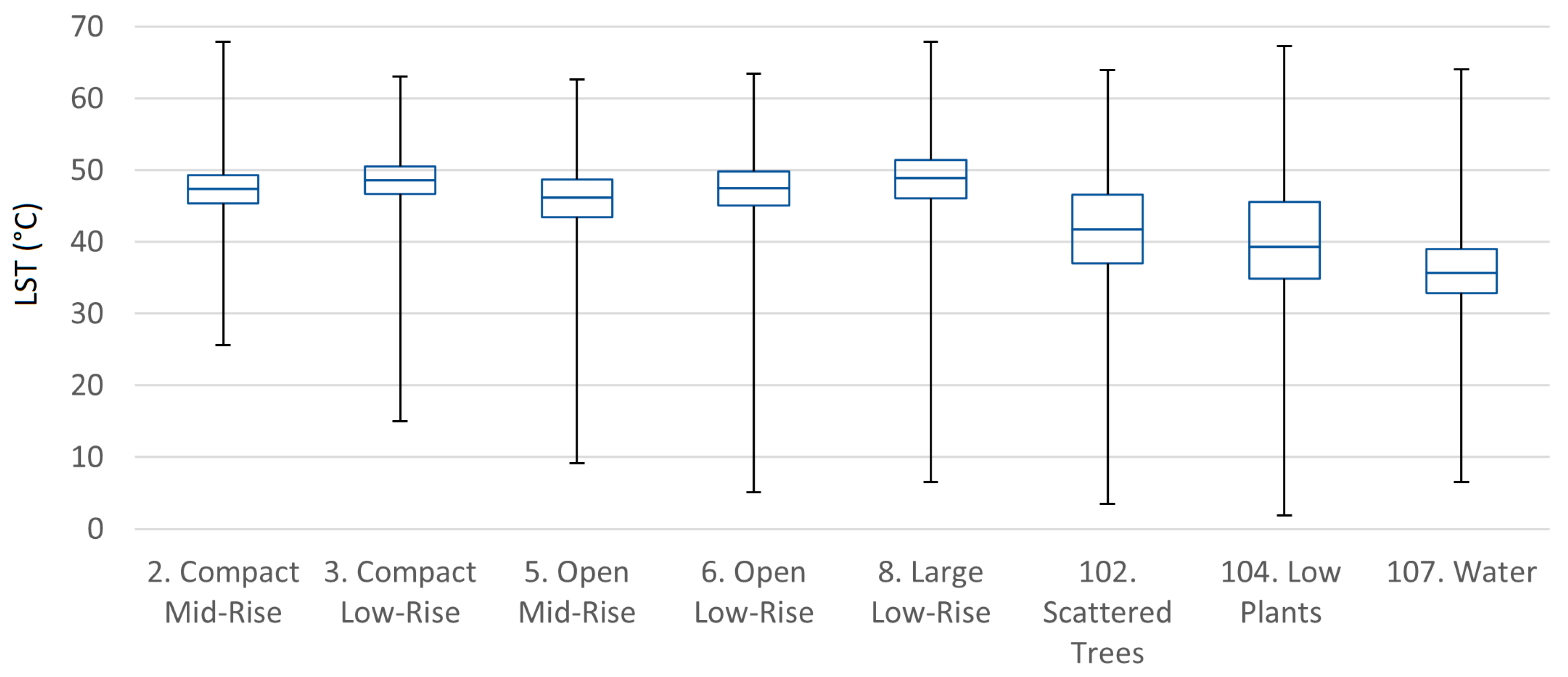
Four LST maps relative to summers 2021 and 2022 (see Figure 8) were computed and used to investigate the variation of LST between the different LCZs. Despite the limited number of images used, the LST maps provided a sufficiently numerous pixel sample to carry out a robust statistical investigation of LST per LCZ. The different temperature patterns depicted in the four maps may be due either to the different atmospheric conditions experienced on the different dates as well as to the presence of cloud spots that were not correctly identified and removed. However, LST patterns in the different land cover types are similar, with vegetated areas exhibiting lower temperature values than densely urbanized surfaces. The main statistics of LST per LCZ were summarized through boxplots as depicted in Figure 9. Built-up classes exhibit higher mean temperatures, ranging between 45.9 °C and 48.5 °C, than non-built-up zones, where average temperatures range between 36.1 °C and 41.8 °C. Given the large dispersion of temperature values within each LCZ class, the surface temperature differences between artificial and natural classes and within the different built-up areas were further investigated.
The first experiment consisted of merging the LCZ classes into two separate groups, namely “natural” and “artificial” areas. Statistics computed for the two macro-classes show that natural areas exhibit a mean LST of 40.3 °C in the considered dates and times, which is 6.7 °C lower than the temperature experienced across the built-up areas in the same time frame (see Table 4). The statistical significance of this difference was checked through a z-test with a significance level of 5%, which resulted in a z-score of 403.3 corresponding to an extremely low p-value. This result suggests rejecting the null hypothesis of equal means and indicates a statistically significant difference between the LST of natural and artificial areas. The Cohen’s d and the CIs were computed to verify the practical significance of the result. The obtained d-value of 0.94 indicates a large effect size, pointing out the mean LST of the built-up group being 0.94 standard deviations above the natural classes’ one. In addition, the difference between the two means was found to be at 95% probability between 6.71 °C and 6.75 °C. These results provide additional pieces of evidence of the ability of natural surfaces to buffering surface temperature values.
In the second experiment, the LST patterns within the artificial surface types were investigated to derive additional considerations on the local effects of urban morphology and land cover on the surface temperature distribution. Table 5 depicts LST mean and standard deviation values for the different built-up classes. Compact Low-Rise (class 3) and Large Low-Rise (class 8) exhibit the highest LST with a mean of 48.5 °C, while the Open Mid-Rise (class 5) ended up with the lowest mean value, 2.6 °C below. Intermediate values were found for Compact Mid-Rise (class 2) and Open Low-Rise (class 6), where mean LST equals 47.1 °C and 47.3 °C, respectively. As in the previous experiment, the statistical and practical significance of such temperature differences were examined.
The ANOVA test was used as a powerful tool to investigate the statistical significance in the case of more than two data categories. Since the hypothesis of homogeneity of variance in the distribution is not met, the Welch’s ANOVA test was used as an alternative. The low p-value (<0.05) proves the statistical significance of the difference between the mean temperatures.
The practical significance of the result was checked by comparing the temperature difference between each pair of built-up classes. Table 6 summarizes the Cohen’s d values, the corresponding effect size, and the 95% CIs of the mean temperature difference for each pair. Medium effect size was revealed for the temperature difference between Compact Low-Rise and Open Mid-Rise as well as Open Mid-Rise and Large Low-Rise. With a mean LST difference ranging from 2.6 °C to 2.7 °C, higher temperatures were experienced in the Compact and Large Low-Rise zones. This could be explained by the fact that, in contrast to classes 3 and 8, class 5 contains mid-rise buildings that introduce shadows onto the urban surfaces, thus contributing to lowering the LST values. In addition, class 8 corresponds to a paved, impervious surface, which significantly reduces the percentage of the permeable area and prevents the decrease of LST. On their side, all the other pairs exhibited similar behavior, with a Cohen’s d suggesting small or very small effects.
These results point out two main factors contributing to the LST decrease in the urban environment: the presence of vegetation and the height of buildings. Indeed, vegetated areas with mid-rise buildings (Open Mid-Rise) experience the lowest average LST, whereas impervious surfaces with low-rise buildings (Compact Low-Rise and Large Low-Rise) exhibit the highest mean LST. Intermediate LST values are recorded across impervious surfaces with medium-sized buildings (Compact Mid-Rise) as well as vegetated areas with mostly low-rise buildings (Open Low-Rise). This suggests that the presence of vegetation may compensate for the lack of high buildings and vice versa.
A further consideration concerning the building density is in order: results show that building density does not play a significant role in the LST distribution. In fact, classes 5 and 8 show very different LST values despite being both characterized by low-density buildings. In contrast, classes 3 and 6, which only differ in the density of their buildings, experience a similar LST, and a small effect size for the LST difference is recorded.

4.3. Correlation between LST and Air Temperature

The temporal correlation between LST and air temperature was assessed over the period 2018–2021, considering the ARPA and Netatmo stations’ measurements separately. The obtained Pearson’s coefficients range from 0.91 to 0.99 for the former, and from 0.85 to 0.99 for the latter, revealing a strong linear correlation between the two temperatures. This result agrees with the findings reported in [62,64].
On the other hand, the spatial correlation between LST and air temperature was computed for the 6th and the 22nd of July 2021, which resulted in a very low Pearson’s coefficient of 0.1 for both dates. When considering only the official ARPA station measurements, this value turned out to be even lower (i.e., 0.01 and −0.04 for 22nd and 6th July, respectively), confirming that no spatial correlation exists between the two variables. For this reason, the LST distribution may not be representative of the actual air temperature patterns in the different LCZs. In contrast, the urban morphology and the land cover composition may have a different influence on the two variables. The combined analysis LST and air temperature is therefore justified when studying the effects of urban morphology and land cover on the local climate.

4.4. Air Temperature per LCZ

ARPA and Netatmo measurements from January 2018 to December 2021 were also exploited to investigate the air temperature variation between the LCZs. Computations were carried out considering all the air temperature observations available per day. Table 7 reports the number of stations per class and highlights the lack of devices, and therefore of records, in natural areas. Consequently, measurements recorded across natural classes are not sufficient to draw meaningful conclusions in this study. Only data measured within the artificial classes were therefore exploited for the analysis.
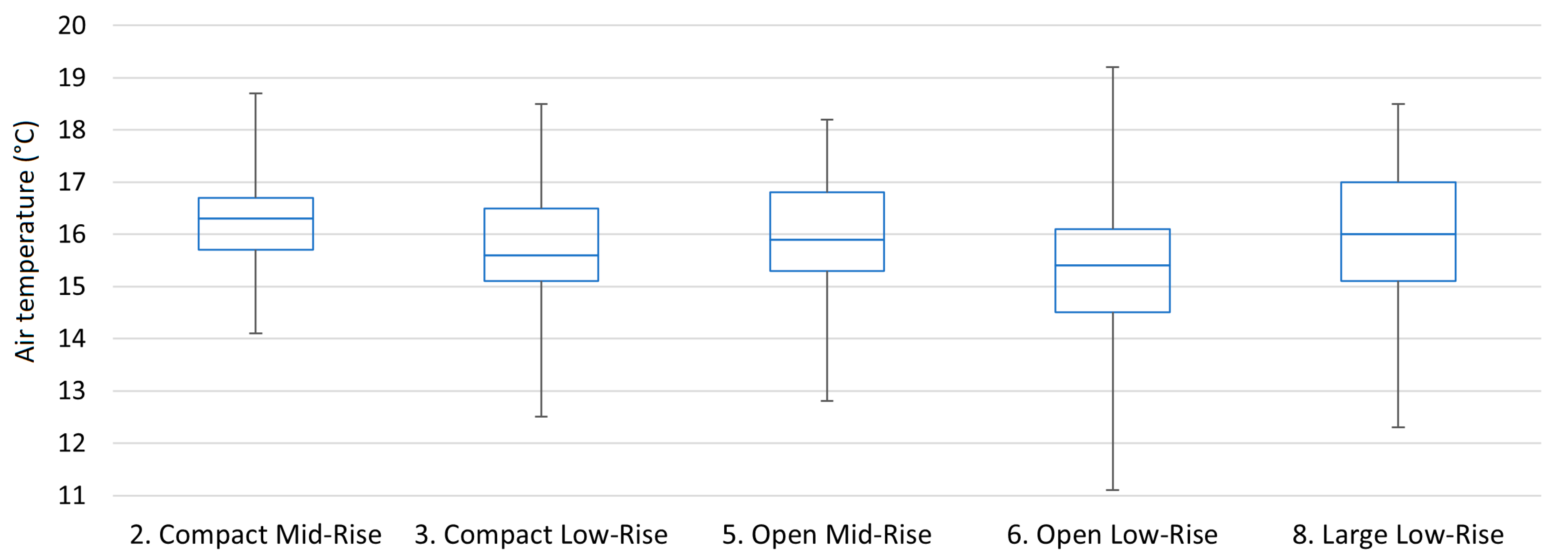
Results obtained in the first experiment, considering the whole study period without seasonal distinctions, are reported in Figure 10. The Open Low-Rise area (class 6), which is characterized by the presence of vegetation and small, low-density buildings, turned out to be the coolest artificial class with a mean air temperature of 15.3 °C. In turn, the Compact Mid-Rise zones (class 2), encompassing impervious areas with high-density, medium-sized buildings, experienced the highest air temperature in the study period, with 1.0 °C higher mean temperature. In between, the Compact Low-Rise (class 3), Large Low-Rise (class 8), and Open Mid-Rise (class 5) areas were found to experience similar mean temperatures, i.e., 15.7 °C, 15.9 °C, and 16.0 °C, respectively. The former two classes comprise non-vegetated areas with small buildings, while the latter includes urban areas with mid-rise buildings and more prominent vegetation. These results point out building density and height as major contributors to the air temperature increase while suggesting vegetation as the main mitigating factor of urban air temperatures.
Given these first pieces of evidence, the significance of the observed temperature differences in the LCZ built-up types was tested as well as the effect size of the three main factors influencing the air temperature distribution. Firstly, the one-way ANOVA resulted in a small p-value (5.83 × 10⁻⁸), which suggests rejecting the hypothesis of equal means with a 5% significance level. To detect the LCZ classes with statistically significant mean temperature differences, several t-tests were performed on each pair of classes. The resulting p-values and the underlying decisions with respect to the null hypothesis of equal means ( H 0 ) are reported in Table 8, together with the Cohen’s d and the corresponding effect size.
By looking at the results of the t-tests, a significant mean air temperature difference was found between Compact Mid-Rise and Open Low-Rise (equal to 0.96 °C), Open Mid-Rise and Open Low-Rise (0.65 °C), and Large Low-Rise and Open Low-Rise (0.62 °C). These outcomes confirm the different effects of building height, which contributes to increase air temperature, and vegetation, which tends to decrease air temperature, on the urban climate. This evidence is reinforced by the significant difference found between Compact Low-Rise and Compact Mid-Rise, which only differ in the height of buildings. A statistically significant difference in air temperature (equal to 0.38 °C) was also found between Compact Low-Rise and Open Low-Rise, pointing out that building density tends to increase local air temperatures; however, given the small effect size, the influence of this factor may be relatively low.
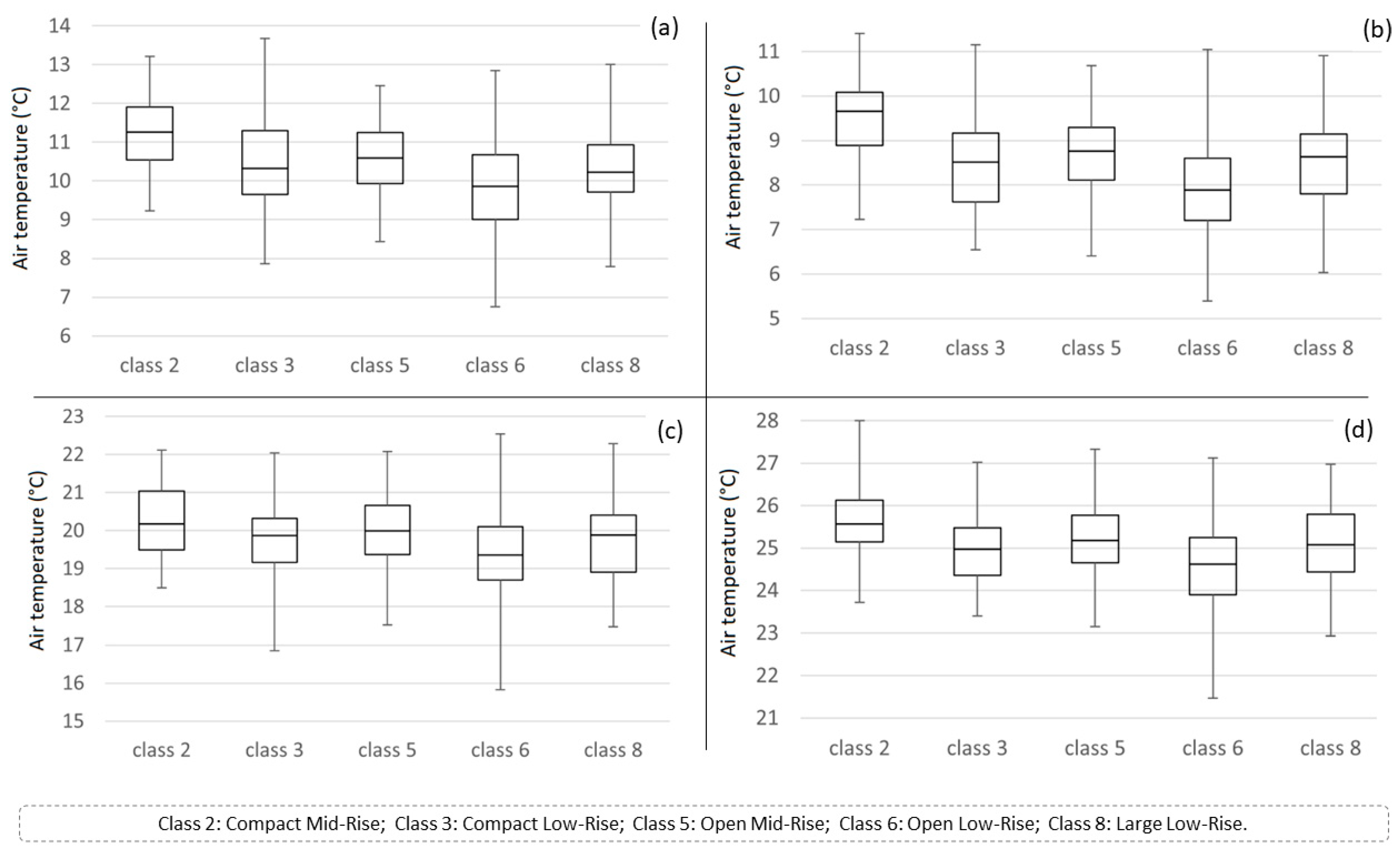
In a second phase, the same tests were carried out for the same period considering each season separately. Figure 11 depicts the boxplots summarizing the air temperature statistics for the four seasons. Table 9 reports the mean air temperature difference, the decision associated with the t-test and the Cohen’s d for all pairs of built-up classes. Results confirm the same built-up classes experiencing the highest and lowest mean air temperatures in every season, namely Compact Mid-Rise and Open Low-Rise, respectively. A greater mean difference is recorded during winter (1.6 °C), autumn (1.3 °C), and summer (1.1 °C). Nonetheless, more pairs than in the previous experiment were found to be statistically different as shown by the cells in bold in Table 9. This is the case of classes Compact Mid-Rise and Large Low-Rise with an effect size ranging from “medium” to “large”, which reinforces the evidence of a warming effect of building height in each season as well. Similarly, a wider difference between Compact Mid-Rise and Open Mid-Rise areas was found for all seasons except spring, with an effect size varying from small in summer, to medium in autumn, to large in winter. Since the building density is the only characteristic differentiating the two classes, this feature turns out to have a greater warming effect during cooler periods. Moreover, for spring and summer, a statistically significant lower mean temperature was found in the Compact Low-Rise class with respect to the Open Mid-Rise class, despite the latter being characterized by the presence of vegetation and less building density. This means that, during warm, vegetative periods, the building height factor contributes to lowering air temperature more than building density and the presence of vegetation.
To sum up, the analysis of air temperature per built-up type pointed out three main mitigating factors of urban air temperatures: presence of vegetation, reduced building height, and reduced building density. Indeed, the coolest and warmest temperature values are experienced by the Open Low-Rise and Compact Mid-Rise LCZs, regardless of the considered period. Results disclosed a mean temperature difference of 1.0°C between said classes. However, the magnitude of air temperature decrease induced by the three mitigating factors is different depending on the season. Specifically, the effect of vegetation and building height generally prevails on the effect of building density; yet, the impact of building density becomes more relevant than the others during summer, autumn, and winter.

5. Discussion and Conclusions

In this paper, the influence of urban morphology and land cover composition on the urban climate of the Metropolitan City of Milan was presented. Satellite imagery and multiple open geo-data were leveraged to achieve a segmentation of the study area in LCZs, taking into account the seasonal variations of vegetation and land cover in a single map (relative to the year 2021). Two climate-related variables, namely LST and air temperature, were considered as a proxy of the local climate conditions. Remotely sensed thermal data (relative to summers 2021 and 2022) was exploited to compute the LST distribution across the study area, while ground-based sensor time series (for the period 2018–2021) collected by both authoritative and crowdsourcing weather networks were used for the analysis of air temperature. Several experiments including statistical tests were carried out to study the underlying relationship between the LCZs and the two temperature variables as well as assess the space-time correlation between LST and air temperature.
The first result in terms of LCZ classification pointed out a good performance of the proposed classification workflow, confirming the benefits provided by the building height dataset for improving classification accuracy, as suggested in [55]. The LCZ mapping protocol defined within the WUDAPT project was here slightly modified by adding a post-processing phase consisting in the application of majority voting to five different LCZ maps. This allowed to further improve classification accuracy as well as provide a more comprehensive view of the seasonal variations of land cover composition in a single LCZ map. With an OA of 94%, the LCZ classification obtained in this work is among the best-quality LCZ maps existing within the WUDAPT database, where only 3% of the available maps have accuracy values higher than 90% [17]. Comparable results were achieved in [55], with OA of 88% and 92% using the Convolutional Neural Network and RF classifiers, respectively.
As for the temperature analysis, despite a strong temporal correlation between LST and air temperature, no spatial correlation between the two variables was found. Several studies reported similar results in terms of temporal correlation, e.g., [30,31], with values ranging between 0.83 and 0.99; however, far fewer studies focused on the assessment of the spatial correlation between the two variables. The implication of these results is twofold. First, they confirm the intuition that remotely sensed LST data cannot be extensively used as a proxy of air temperature, whose spatial distribution should be assessed through ground-based sensing networks. Furthermore, they justify the separate investigations of the two temperature variables that were carried out in this study. These considerations are in agreement with the findings of [60], where the authors pointed out the importance of both land surface and air temperatures as complementary valuable information for climate-related studies.
Experiments disclosed an underlying relationship between urban morphology (in terms of urban structure and land cover) and urban temperatures (both land surface and air temperatures). Specifically, comparing the outcomes obtained from the different tests, vegetation turned out to be a common mitigating factor of both temperatures, a result that is widely accepted in the literature [65,66,67]. Contrarily, this consensus is not always found when considering other temperature-buffering factors. Indeed, in this study the building height was found to reduce the LST by creating shadows on the ground while contributing to increasing air temperature owing to heat storage and reduced local air circulation. This is in line with [65,68], in which the authors pointed out that lower LST values are recorded in low-rise building areas; however, it is opposite to the findings of [69], where a positive correlation between LST and building height is reported. Furthermore, in the present work the density of buildings resulted to have a way lower influence on the urban climate, leading to a slight increase in air temperature while not significantly influencing the LST. Although this result agrees with the outcomes of [27], where the most intense cooling effect was found in open-set and sparsely built-up regions in all seasons, some other studies came up with different conclusions. For instance, LST may increase with decreasing building density [70], and densely urbanized areas may create local cool islands [71], Nonetheless, these differences may be justified considering that the same factor can have significantly different effects on the local thermal conditions mainly depending on the background climate [2] suggesting that it is difficult to draw general conclusions which apply to cities worldwide.
The combined use of global coverage data such as Landsat 8 imagery with in situ temperature measurements and geospatial databases (typically provided by local authorities) enables the replicability of the analysis to other case studies. Concerns on the availability of open building height datasets have to be pointed out; however, this limitation may be overcome by using the building height layer distributed by Copernicus within the Urban Atlas product. Moreover, the crowdsourced data exploited in this work were key for increasing the spatial coverage of air temperature measurements, allowing for a more insightful investigation of its space-time patterns. Despite the undeniable advantages of crowdsourced observations, data cleaning is a crucial step that may significantly reduce the number of usable observations, as highlighted also in [34]. Thus, this study proves that the integration of crowdsourced observations with official measurements may be beneficial for urban climate analyses, provided that a suitable data cleaning pre-processing is carried out. In this context, starting from the pieces of code developed within this study, the implementation of a Python application enabling a semi-automatic pre-processing of Netatmo data is foreseen as a future development of this work. This would ensure a straightforward usage of Netatmo measurements to many other applications and cases of study, given the network’s worldwide coverage.
The approach looks promising for investigating UHI effect and urban climate at the local scale. Maps, exploratory graphs, and tables produced in this work represent crucial tools to drive evidence-based policies connected to urban planning and design as well as urban climate monitoring.

Author Contributions

Conceptualization, M.P., A.V. and M.A.B.; methodology, M.P., A.V. and M.A.B.; software, M.P. and A.V.; validation, M.P. and A.V.; investigation, M.P.; data curation, M.P.; writing—original draft, M.P. and A.V.; writing—review and editing, M.P., A.V. and M.A.B.; visualization, M.P.; supervision, M.A.B.; project administration, M.A.B. All authors have read and agreed to the published version of the manuscript.

Funding

This research has been partially funded by the EU Horizon 2020 project “HARMONIA” (ID H2020-LC-CLA-2018-2019-2020, GA No. 101003517).

Data Availability Statement

No new data were created or analyzed in this study. Data sharing is not applicable to this article.

Acknowledgments

The paper is based on open and free datasets (Landsat 8 imagery, land consumption data, topographic database, and air temperature observations). The authors would like to gratefully acknowledge data providers (United States Geological Survey—USGS, Istituto Superiore per la Protezione e la Ricerca Ambientale—ISPRA, Regione Lombardia, Agenzia Regionale per la Protezione dell’Ambiente—ARPA Lombardia, and Netatmo).

Conflicts of Interest

The authors declare no conflict of interest.

References

  1. United Nations. World Urbanization Prospects: The 2020 Revision. Available online: https://www.worldbank.org/en/topic/urbandevelopment/overview (accessed on 3 October 2022).
  2. European Environment Agency. Urban Sustainability: How Can Cities Become Sustainable? Available online: https://www.eea.europa.eu/themes/sustainability-transitions/urban-environment (accessed on 3 October 2022).
  3. Gurney, K.R.; Romero-Lankao, P.; Seto, K.C.; Hutyra, L.R.; Duren, R.; Kennedy, C.; Grimm, N.B.; Ehleringer, J.R.; Marcotullio, P.; Hughes, S.; et al. Climate change: Track urban emissions on a human scale. Nature 2015, 525, 179–181. [Google Scholar] [CrossRef] [Green Version]
  4. Creutzig, F.; Agoston, P.; Minx, J.C.; Canadell, J.G.; Andrew, R.M.; Le Quéré, C.; Peters, G.P.; Sharifi, A.; Yamagata, Y.; Dhakal, S. Urban infrastructure choices structure climate solutions. Nature Clim. Change 2016, 6, 1054–1056. [Google Scholar] [CrossRef]
  5. Gasparini, P.; Di Ruocco, A.; Russo, R. Natural Hazards Impacting on Future Cities. In Resilience and Sustainability in Relation to Natural Disasters: A Challenge for Future Cities; Gasparini, P., Manfredi, G., Asprone, D., Eds.; Springer: Cham, Switzerland, 2014. [Google Scholar] [CrossRef]
  6. Intergovernmental Panel on Climate Change. Summary for Policymakers. In Climate Change 2014: Mitigation of Climate Change: Working Group III Contribution to the IPCC Fifth Assessment Report; Cambridge University Press: Cambridge, UK, 2015; pp. 1–30. [Google Scholar] [CrossRef]
  7. Chapman, S.; Thatcher, M.; Salazar, A.; Watson, J.E.M.; McAlpine, C.A. The impact of climate change and urban growth on urban climate and heat stress in a subtropical city. Int. J. Climatol. 2019, 39, 3013–3030. [Google Scholar] [CrossRef] [Green Version]
  8. Salazar, A.; Baldi, G.; Hirota, M.; Syktus, J.; McAlpine, C. Land use and land cover change impacts on the regional climate of non-Amazonian South America: A review. Glob. Planet. Change 2015, 128, 103–119. [Google Scholar] [CrossRef]
  9. NASA. ARSET Satellite Remote Sensing for Urban Heat Islands. Available online: https://appliedsciences.nasa.gov/join-mission/training/english/arset-satellite-remote-sensing-urban-heat-islands (accessed on 5 October 2022).
  10. McCarthy, M.P.; Best, M.J.; Betts, R.A. Climate change in cities due to global warming and urban effects. Geophys. Res. Lett. 2010, 37, L09705. [Google Scholar] [CrossRef] [Green Version]
  11. Oke, T.R.; Mills, G.; Christen, A.; Voogt, J.A. Urban Climates; Cambridge University Press: Cambridge, UK, 2017. [Google Scholar] [CrossRef] [Green Version]
  12. Shao, M.; Tang, X.; Zhang, Y.; Li, W. City clusters in China: Air and surface water pollution. Front. Ecol. Environ. 2006, 4, 353–361. [Google Scholar] [CrossRef]
  13. de Almeida, C.R.; Teodoro, A.C.; Gonçalves, A. Study of the Urban Heat Island (UHI) Using Remote Sensing Data/Techniques: A Systematic Review. Environments 2021, 8, 105. [Google Scholar] [CrossRef]
  14. Stewart, I.D.; Oke, T.R. Local climate zones for urban temperature studies. Bull. Am. Meteorol. Soc. 2012, 93, 1879–1900. [Google Scholar] [CrossRef]
  15. Zhao, C.; Jensen, J.L.R.; Weng, Q.; Currit, N.; Weaver, R. Use of Local Climate Zones to investigate surface urban heat islands in Texas. GISci. Remote Sens. 2020, 57, 1083–1101. [Google Scholar] [CrossRef]
  16. Long, N.; Gardes, T.; Hidalgo, J.; Masson, V.; Schoetter, R. Influence of the urban morphology on the urban heat island intensity: An approach based on the Local Climate Zone classification. PeerJ 2018, 6, e27208v1. [Google Scholar] [CrossRef]
  17. WUDAPT. World Urban Database. Available online: http://www.wudapt.org (accessed on 6 October 2022).
  18. Bechtel, B.; Alexander, P.; Böhner, J.; Ching, J.; Conrad, O.; Feddema, J.; Mills, G.; See, L.; Stewart, I. Mapping local climate zones for a worldwide database of the form and function of cities. ISPRS Int. J. Geo-Inf. 2015, 4, 199–219. [Google Scholar] [CrossRef] [Green Version]
  19. Urban, M.; Eberle, J.; Hüttich, C.; Schmullius, C.; Herold, M. Comparison of Satellite-Derived Land Surface Temperature and Air Temperature from Meteorological Stations on the Pan-Arctic Scale. Remote Sens. 2013, 5, 2348–2367. [Google Scholar] [CrossRef] [Green Version]
  20. Mutiibwa, D.; Strachan, S.; Albright, T. Land surface temperature and surface air temperature in complex terrain. IEEE J. Sel. Top. Appl. Earth Obs. Remote Sens. 2015, 8, 4762–4774. [Google Scholar] [CrossRef]
  21. Schwarz, N.; Schlink, U.; Franck, U.; Großmann, K. Relationship of land surface and air temperatures and its implications for quantifying urban heat island indicators—An application for the city of Leipzig (Germany). Ecol. Indic. 2012, 18, 693–704. [Google Scholar] [CrossRef]
  22. Cai, M.; Ren, C.; Xu, Y.; Lau, K.K.L.; Wang, R. Investigating the relationship between local climate zone and land surface temperature using an improved WUDAPT methodology—A case study of Yangtze River Delta, China. Urban Clim. 2018, 24, 485–502. [Google Scholar] [CrossRef]
  23. Geletič, J.; Lehnert, M.; Dobrovolný, P. Land Surface Temperature Differences within Local Climate Zones, Based on Two Central European Cities. Remote Sens. 2016, 8, 788. [Google Scholar] [CrossRef] [Green Version]
  24. Alexander, P.J.; Mills, G. Local Climate Classification and Dublin’s Urban Heat Island. Atmosphere 2014, 5, 755–774. [Google Scholar] [CrossRef] [Green Version]
  25. Su, Y.; Wu, J.; Zhang, C.; Wu, X.; Li, Q.; Liu, L.; Bi, C.; Zhang, H.; Lafortezza, R.; Chen, X. Estimating the cooling effect magnitude of urban vegetation in different climate zones using multi-source remote sensing. Urban Clim. 2022, 43, 101155. [Google Scholar] [CrossRef]
  26. Leconte, F.; Bouyer, J.; Claverie, R.; Pétrissans, M. Using Local Climate Zone scheme for UHI assessment: Evaluation of the method using mobile measurements. Build. Environ. 2015, 83, 39–49. [Google Scholar] [CrossRef]
  27. Thomas, G.; Sherin, A.P.; Ansar, S.; Zachariah, E.J. Analysis of Urban Heat Island in Kochi, India, Using a Modified Local Climate Zone Classification. Procedia Environ. Sci. 2014, 21, 3–13. [Google Scholar] [CrossRef] [Green Version]
  28. Vancutsem, C.; Ceccato, P.; Dinku, T.; Connor, S.J. Evaluation of MODIS land surface temperature data to estimate air temperature in different ecosystems over Africa. Remote Sens. Environ. 2010, 114, 449–465. [Google Scholar] [CrossRef]
  29. Prihodko, L.; Goward, S.N. Estimation of air temperature from remotely sensed surface observations. Remote Sens. Environ. 1997, 60, 335–346. [Google Scholar] [CrossRef]
  30. Zhu, W.; Lű, A.; Jia, S. Estimation of daily maximum and minimum air temperature using MODIS land surface temperature products. Remote Sens. Environ. 2013, 130, 62–73. [Google Scholar] [CrossRef]
  31. Shen, S.; Leptoukh, G.G. Estimation of surface air temperature over central and eastern Eurasia from MODIS land surface temperature. Environ. Res. Lett. 2011, 6, 045206. [Google Scholar] [CrossRef]
  32. Lotfian, M.; Ingensand, J.; Brovelli, M.A. A Framework for Classifying Participant Motivation that Considers the Typology of Citizen Science Projects. ISPRS Int. J. Geo-Inf. 2020, 9, 704. [Google Scholar] [CrossRef]
  33. Zumwald, M.; Knüsel, B.; Bresch, D.N.; Knutti, R. Mapping urban temperature using crowd-sensing data and machine learning. Urban Clim. 2021, 35, 100739. [Google Scholar] [CrossRef]
  34. Meier, F.; Fenner, D.; Grassmann, T.; Otto, M.; Scherer, D. Crowdsourcing air temperature from citizen weather stations for urban climate research. Urban Clim. 2017, 19, 170–191. [Google Scholar] [CrossRef]
  35. Napoly, A.; Grassmann, T.; Meier, F.; Fenner, D. Development and Application of a Statistically-Based Quality Control for Crowdsourced Air Temperature Data. Front. Earth Sci. 2018, 6, 118. [Google Scholar] [CrossRef] [Green Version]
  36. Oxoli, D.; Ronchetti, G.; Minghini, M.; Molinari, M.E.; Lotfian, M.; Sona, G.; Brovelli, M.A. Measuring Urban Land Cover Influence on Air Temperature through Multiple Geo-Data—The Case of Milan, Italy. ISPRS Int. J. Geo-Inf. 2018, 7, 421. [Google Scholar] [CrossRef] [Green Version]
  37. Eurostat. Population on 1 January by Age Groups and Sex—Cities and Grater Cities. Available online: https://ec.europa.eu/eurostat/web/products-datasets/-/urb_cpop1 (accessed on 16 October 2022).
  38. Köppen, W. Die Wärmezonen der Erde, nach der Dauer der heissen, gemässigten und kalten Zeit und nach der Wirkung der Wärme auf die organische Welt betrachtet. Meteorol. Zeitsch. 1884, 1, 5–226. [Google Scholar]
  39. Aeronautica Militare. Tabelle Climatiche 1971–2000 della Stazione Meteorologica di Milano Linate dall’Atlante Climatico 1971–2000 del Servizio Meteorologico dell’Aeronautica Militare. Available online: http://www.meteoam.it/ (accessed on 16 October 2022).
  40. Pichierri, M.; Bonafoni, S.; Biondi, R. Satellite air temperature estimation for monitoring the canopy layer heat island of Milan. Remote Sens. Environ. 2012, 127, 130–138. [Google Scholar] [CrossRef]
  41. Bacci, P.; Maugeri, M. The urban heat island of Milan. Nuovo Cim. C 1992, 15, 417–424. [Google Scholar] [CrossRef]
  42. ISPRA. Consumo di Suolo. Available online: https://groupware.sinanet.isprambiente.it/uso-copertura-e-consumo-di-suolo/library/consumo-di-suolo (accessed on 17 October 2022).
  43. García, D.H. Analysis and precision of the Terrestrial Surface Temperature using Landsat 8 and Sentinel 3 images: Study applied to the city of Granada (Spain). Sustain. Cities Soc. 2021, 71, 102980. [Google Scholar] [CrossRef]
  44. Regione Lombardia. Database Topografico Regionale (DBTR). Available online: http://www.geoportale.regione.lombardia.it/download-dati (accessed on 19 October 2022).
  45. QuickMapServices Plugin. GitHub Repository. Available online: https://github.com/nextgis/quickmapservices (accessed on 2 November 2022).
  46. Open Data Regione Lombardia. Dati Sensori Meteo. Available online: https://www.dati.lombardia.it/browse?q=Dati%20sensori%20meteo&sortBy=relevance (accessed on 19 October 2022).
  47. Netatmo. Official Home Page. Available online: https://www.netatmo.com/en-us (accessed on 19 October 2022).
  48. Python Documentation. Patatmo. Available online: https://nobodyinperson.gitlab.io/python3-patatmo/ (accessed on 19 October 2022).
  49. Python Documentation. Pandas. Available online: https://pandas.pydata.org/docs/ (accessed on 20 October 2022).
  50. Python Documentation. Fiona. Available online: https://fiona.readthedocs.io/en/latest/ (accessed on 20 October 2022).
  51. R Documentation. Raster. Available online: https://www.rdocumentation.org/packages/raster/versions/3.6-3 (accessed on 20 October 2022).
  52. R Documentation. RandomForest. Available online: https://www.rdocumentation.org/packages/randomForest/versions/4.7-1.1/topics/randomForest (accessed on 20 October 2022).
  53. Lotfian, M. Urban Climate Modelling, Case Study of Milan City. Master’s Thesis, Politecnico di Milano, Milan, Italy, 2016. Available online: http://hdl.handle.net/10589/125023 (accessed on 14 November 2022).
  54. Horning, N. Random Forests: An Algorithm for Image Classification and Generation of Continuous Fields Data Sets. In Proceedings of the International Conference on Geoinformatics for Spatial Infrastructure Development in Earth and Allied Sciences, Osaka, Japan, 9–11 December 2010. [Google Scholar]
  55. Fung, K.Y.; Yang, Z.-L.; Niyogi, D. Improving the local climate zone classification with building height, imperviousness, and machine learning for urban models. Computat. Urban Sci. 2022, 2, 16. [Google Scholar] [CrossRef] [PubMed]
  56. CloudMasking Plugin. GitHub Repository. Available online: https://github.com/SMByC/CloudMasking (accessed on 1 November 2022).
  57. Cook, M.; Schott, J.R.; Mandel, J.; Raqueno, N. Development of an Operational Calibration Methodology for the Landsat Thermal Data Archive and Initial Testing of the Atmospheric Compensation Component of a Land Surface Temperature (LST) Product from the Archive. Remote Sens. 2014, 6, 11244–11266. [Google Scholar] [CrossRef] [Green Version]
  58. Lin, M.; Lucas, H.; Shmueli, G. Too Big to Fail: Large Samples and the p-Value Problem. Inf. Syst. Res. 2013, 24, 906–917. [Google Scholar] [CrossRef] [Green Version]
  59. Cohen, J. Statistical Power Analysis for the Behavioral Sciences; Academic Press: Cambridge, MA, USA, 1977. [Google Scholar] [CrossRef]
  60. Jin, M.S.; Dickinson, R.E. Land surface skin temperature climatology: Benefitting from the strengths of satellite observations. Environ. Res. Lett. 2010, 5, 044004. [Google Scholar] [CrossRef] [Green Version]
  61. do Nascimento, A.C.L.; Galvani, E.; Gobo, J.P.A.; Wollmann, C.A. Comparison between Air Temperature and Land Surface Temperature for the City of São Paulo, Brazil. Atmosphere 2022, 13, 491. [Google Scholar] [CrossRef]
  62. Iqbal, B.; Ali, M. Estimation of spatio-temporal air temperature from satellite based LST under semi-arid to arid environment in Peshawar Basin, Northwest Pakistan. Adv. Space Res. 2022, 70, 961–975. [Google Scholar] [CrossRef]
  63. Copernicus Land Monitoring Service. Building Height. 2012. Available online: https://land.copernicus.eu/local/urban-atlas/building-height-2012 (accessed on 1 November 2022).
  64. Colombi, A.; De Michele, C.; Pepe, M.; Rampini, A.; Michele, C.D. Estimation of daily mean air temperature from MODIS LST in Alpine areas. EARSeL eProc. 2007, 6, 38–46. [Google Scholar]
  65. Wang, Y.; Zhan, Q.; Ouyang, W. Impact of Urban Climate Landscape Patterns on Land Surface Temperature in Wuhan, China. Sustainability 2017, 9, 1700. [Google Scholar] [CrossRef] [Green Version]
  66. Tse, J.W.P.; Yeung, P.S.; Fung, J.-C.-H.; Ren, C.; Wang, R.; Wong, M.-M.-F.; Cai, M. Investigation of the meteorological effects of urbanization in recent decades: A case study of major cities in Pearl River Delta. Urban Clim. 2018, 26, 174–187. [Google Scholar] [CrossRef]
  67. Das, M.; Das, A. Assessing the relationship between local climatic zones (LCZs) and land surface temperature (LST)—A case study of Sriniketan–Santiniketan Planning Area (SSPA), West Bengal, India. Urban Clim. 2020, 32, 100591. [Google Scholar] [CrossRef]
  68. Yang, J.; Ren, J.; Sun, D.; Xiao, X.; Xia, J.; Jin, C.; Li, X. Understanding land surface temperature impact factors based on local climate zones. Sustain. Cities Soc. 2021, 69, 102818. [Google Scholar] [CrossRef]
  69. Mushore, T.D.; Dube, T.; Manjowe, M.; Gumindoga, W.; Chemura, A.; Rousta, I.; Odindi, J.; Mutanga, O. Remotely sensed retrieval of Local Climate Zones and their linkages to land surface temperature in Harare metropolitan city, Zimbabwe. Urban Clim. 2019, 27, 259–271. [Google Scholar] [CrossRef]
  70. Middel, A.; Häb, K.; Brazel, A.J.; Martin, C.A.; Guhathakurta, S. Impact of urban form and design on mid-afternoon microclimate in Phoenix Local Climate Zones. Landsc. Urban Plan. 2014, 122, 16–28. [Google Scholar] [CrossRef]
  71. Li, N.; Wang, B.; Yao, Y.; Chen, L.; Zhang, Z. Thermal Contribution of the Local Climate Zone and Its Spatial Distribution Effect on Land Surface Temperature in Different Macroclimate Cities. Remote Sens. 2022, 14, 4029. [Google Scholar] [CrossRef]
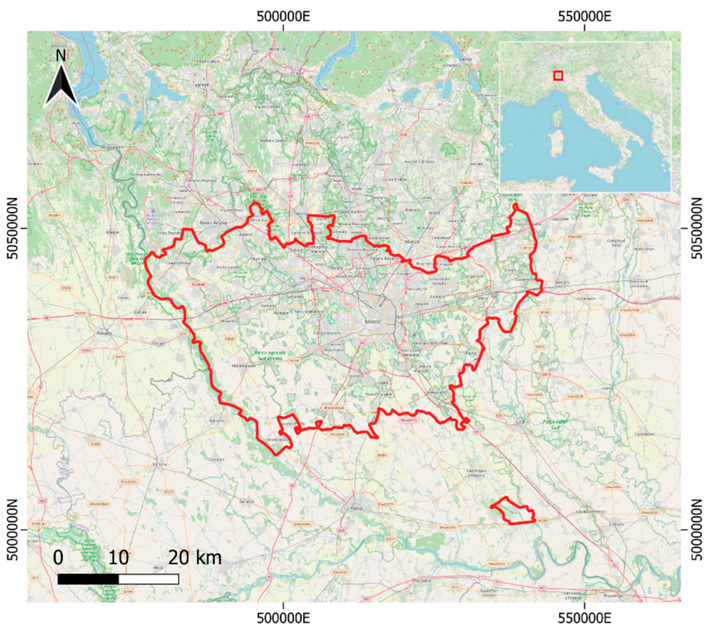
Figure 1. Location of the study area (Metropolitan City of Milan, northern Italy). Coordinate Reference System (CRS): WGS84/UTM zone 32N. Basemap data: © OpenStreetMap contributors.
Remotesensing 15 00733 g001
Figure 2. Locations of Regional Agency for Environmental Protection (ARPA) and Netatmo stations in the study area for the year 2021. CRS: WGS84/UTM zone 32N. Basemap data: © OpenStreetMap Contributors.
Remotesensing 15 00733 g002
Figure 3. Flowchart followed for LCZ mapping from Landsat 8 images.
Remotesensing 15 00733 g003
Figure 4. Flowchart adopted for LST analysis.
Remotesensing 15 00733 g004
Figure 5. ARPA and Netatmo data pre-processing steps.
Remotesensing 15 00733 g005
Figure 6. Flowchart followed for the analysis of the relation between LCZ and air temperature.
Remotesensing 15 00733 g006
Figure 7. The two resulting LCZ maps obtained from Landsat 8 imagery classification: (a) before improvement; (b) after improvement. CRS: WGS84/UTM zone 32N.
Remotesensing 15 00733 g007
Figure 8. LST maps computed from Landsat 8 imagery relative to: (a) 6 July 2021; (b) 22 July 2021; (c) 17 July 2022; (d) 9 July 2022. Cloud-contaminated pixels are removed from the maps. CRS: WGS84/UTM zone 32N.
Remotesensing 15 00733 g008
Figure 9. Boxplots of the LST per LCZ class. Each box is delimited by the first and third quartiles of the distribution. The median is represented as a horizontal line inside each box. The two lines extending from the box (whiskers) describe the distribution variability outside the quartiles.
Remotesensing 15 00733 g009
Figure 10. Boxplots representing the air temperature distribution per LCZ class (considering all the observations available in the period 2018–2021).
Remotesensing 15 00733 g010
Figure 11. Boxplots of air temperature values per class in the four seasons (all observations in the period 2018–2021): (a) autumn, (b) winter, (c) spring, (d) summer.
Remotesensing 15 00733 g011
Table 1. Acquisition date and time for Landsat 8 images used for LCZ and LST mapping. Time is given in Greenwich Mean Time (GMT).
Acquisition Date and Time
For LCZ MappingFor LST Mapping
19 May 2021 10:10 a.m. (spring)5 September 2020 10:10 a.m. (summer)
6 July 2021 10:10 a.m. (summer)6 July 2021 10:10 a.m. (summer)
24 September 2021 10:10 a.m. (autumn)9 July 2021 10:10 a.m. (summer)
5 December 2021 10:10 a.m. (winter)17 July 2022 10:10 a.m. (summer)
16 March 2021 10:10 a.m. (additional image)
Table 2. Description of the LCZ classes identified in the Metropolitan City of Milan.
Class ID and NameClass Definition
2—Compact Mid-RiseDense mix of mid-rise buildings (3–9 stories).
Few or no trees. Land cover mostly paved.
Stone, brick, tile, and concrete construction materials.
3—Compact Low-RiseDense mix of low-rise buildings (1–3 stories).
Few or no trees. Land cover mostly paved.
Stone, brick, tile, and concrete construction materials.
5—Open Mid-RiseOpen arrangement of mid-rise buildings (3–9 stories).
Abundance of pervious land cover (low plants, scattered trees).
Concrete, steel, stone, and glass construction materials.
6—Open Low-RiseOpen arrangement of low-rise buildings (1–3 stories).
Abundance of pervious land cover (low plants, scattered trees).
Wood, brick, stone, tile and concrete construction materials.
8—Large Low-RiseOpen arrangement of large low-rise buildings (1–3 stories).
Few or no trees. Land cover mostly paved.
Steel, concrete, metal, and stone construction materials.
102—Scattered TreesLightly wooded landscape of deciduous and/or evergreen trees.
Land cover mostly pervious (low plants).
Zone function is natural forest, tree cultivation or urban park.
104—Low PlantsFeatureless landscape of grass or herbaceous plants/crops.
Few or no trees.
Zone function is natural grassland, agriculture, or urban park.
107—WaterLarge, open water bodies such as seas and lakes,
or small bodies such as rivers, reservoirs, and lagoons.
Table 3. Accuracies of the LCZ classification output, before and after classification improvement.
ClassBefore ImprovementAfter Improvement
PA (%)UA (%)OA (%)PA (%)UA (%)OA (%)
2—Compact Mid-Rise98.794.594.997.995.794.0
3—Compact Low-Rise60.691.782.889.6
5—Open Mid-Rise62.186.382.594.4
6—Open Low-Rise94.180.890.985.9
8—Large Low-Rise98.096.797.795.1
102—Scattered Trees99.696.599.095.3
104—Low Plants98.699.399.298.5
107—Water100.099.599.499.6
Table 4. LST statistics for artificial and natural classes.
LST Mean (°C)LST Standard Deviation (°C)
Artificial classes
(classes 2, 3, 5, 6, and 8)
47.13.3
Natural classes
(classes 102, 104, and 107)
40.37.3
Table 5. LST statistics for artificial classes.
LST Mean (°C)LST Standard Deviation (°C)
2—Compact Mid-Rise47.13.3
3—Compact Low-Rise48.53.7
5—Open Mid-Rise45.94.2
6—Open Low-Rise47.34.3
8—Large Low-Rise48.54.4
Table 6. Cohen’s d (size effect) and 95% Cis for LST difference between each pair of artificial classes. The letters in parenthesis indicate the corresponding effect size: Negligible (N), Very small (VS), Small (S), Medium (M), Large (L), Very large (VL).
Classes2 and 32 and 52 and 62 and 83 and 53 and 63 and 85 and 65 and 86 and 8
Cohen’s d0.40 (S)0.32 (S)0.06 (VS)0.34 (S)0.65 (M)0.27 (S)0.02 (VS)0.35 (S)0.61 (M)0.28 (S)
CIs (°C)1.38–1.431.19–1.230.24–0.271.45–1.492.59–2.651.12–1.160.04–0.091.46–1.492.67–2.701.19–1.23
Table 7. Number of air temperature stations per LCZ class.
ClassNumber of Stations
2—Compact Mid-Rise49
3—Compact Low-Rise57
5—Open Mid-Rise95
6—Open Low-Rise189
8—Large Low-Rise44
102—Scattered Trees5
104—Low Plants8
107—Water0
Table 8. Results of the t-tests and values of Cohen’s d for each pair of artificial classes (study period 2018–2021).
Classes2 and 32 and 52 and 62 and 83 and 53 and 63 and 85 and 65 and 86 and 8
Δ T  10.560.300.960.330.270.380.230.650.030.62
H 0 (t-test) 2NOOKNOOKOKNOOKNOOKNO
Cohen’s d 30.51 (M)0.28 (S)0.75 (M)0.27 (S)0.24 (S)0.30 (S)0.18 (VS/S)0.52 (M)0.03 (VS)0.47 (S/M)
1 Mean difference of air temperature (°C). 2 Result of the t-test: hypothesis of equal means H 0 rejected (NO, p-value < 0.05) or accepted (OK, p-value ≥ 0.05). 3 Cohen’s d value and corresponding effect size: Negligible (N), Very small (VS), Small (S), Medium (M), Large (L), Very large (VL).
Table 9. Results of the t-tests and values of Cohen’s d for each pair of artificial classes in the four seasons (study period 2018–2021).
Classes2 and 32 and 52 and 62 and 83 and 53 and 63 and 85 and 65 and 86 and 8
Autumn Δ T  10.800.611.290.910.190.480.110.680.300.38
H 0 (t-test) 2NONONONOOKNOOKNOOKNO
Cohen’s d 30.74 (M)0.65 (M)1.17 (L)0.93 (L)0.18 (VS)0.42 (S)0.09 (VS)0.62 (M)0.30 (S)0.34 (S)
Winter Δ T 1.010.801.621.020.210.610.010.830.220.60
H 0 (t-test)NONONONOOKNOOKNOOKNO
Cohen’s d0.96 (L)0.85 (L)1.55 (VL)1.02 (L)0.21 (S)0.56 (M)0.01 (N)0.80 (L)0.23 (S)0.57 (M)
Spring Δ T 0.480.190.830.550.290.350.070.630.360.28
H 0 (t-test)NOOKNONONONOOKNOOKOK
Cohen’s d0.47 (S/M)0.21 (S)0.78 (M)0.54 (M)0.30 (S)0.33 (S)0.07 (VS)0.62 (M)0.37 (S)0.26 (S)
Summer Δ T 0.680.411.030.590.280.350.090.630.180.44
H 0 (t-test)NONONONONONOOKNOOKNO
Cohen’s d0.79 (M/L)0.47 (S)1.09 (L)0.66 (M)0.32 (S)0.37 (S)0.10 (VS)0.67 (M)0.21 (S)0.46 (S)
1 Mean difference of air temperature (°C). 2 Result of the t-test: hypothesis of equal means H 0 rejected (NO, p-value < 0.05) or accepted (OK, p-value ≥ 0.05). Bold indicates that the result is different with respect to what obtained from the analysis of the whole study period. 3 Cohen’s d value and corresponding effect size: Negligible (N), Very small (VS), Small (S), Medium (M), Large (L), Very large (VL).
Disclaimer/Publisher’s Note: The statements, opinions and data contained in all publications are solely those of the individual author(s) and contributor(s) and not of MDPI and/or the editor(s). MDPI and/or the editor(s) disclaim responsibility for any injury to people or property resulting from any ideas, methods, instructions or products referred to in the content.