Detection of Aquatic Invasive Plants in Wetlands of the Upper Mississippi River from UAV Imagery Using Transfer Learning

Abstract

Aquatic invasive plants (AIPs) are a global threat to local biodiversity due to their rapid adaptation to the new environments. Lythrum salicaria, commonly known as purple loosestrife, is a predominant AIP in the upper Midwestern region of the United States and has been designated as a deadly threat to the wetlands of this region. Accurate estimation of its current extent is a top priority, but regular monitoring is limited due to cost-, labor-, and time-intensive field surveys. Therefore, the goal of the present study is to accurately detect purple loosestrife from very high-resolution UAV imagery using deep neural network-based models. As a case study, this study implemented U-Net and LinkNet models with ResNet-152 encoder in the wetlands of the upper Mississippi River situated in La Crosse County, Wisconsin. The results showed that both models produced 88–94% training accuracy and performed better in landscapes that were occupied by smaller, disaggregated, and more equitably distributed purple loosestrife. Furthermore, the study adopted a transfer learning approach to implement a trained purple loosestrife model of the first study site and implemented it for the second study site. The results showed that the pre-trained model implementation generated better accuracy in less than half the time of the original model. Therefore, the transfer learning approach, if adapted efficiently, can be highly beneficial for continuous monitoring of purple loosestrife and strategic planning for application of direct biocontrol measures.

1. Introduction

Aquatic invasive plants (AIPs) (the plant species that spread outside their native range [1]) are a global threat to biodiversity, ecosystem degradation, local economies, and human health [2,3]. AIPs are known for their rapid and effective adaptation to new environments. They benefit from ecosystem changes and habitat disturbances caused by global climatic change and anthropogenic impacts [4]. AIPs degrade the natural local ecosystem by outcompeting native species [5], negatively affecting the waterfront property values [6,7], and hampering commercial and recreational fishing (and associated losses in taxes and economic revenue) [8]. It was estimated that the annual cost of invasive species invasion in the United States increased from USD 2 billion in 1960–1969 to USD 21 billion in 2010–2020 [9]. In the Midwest, the Great Lakes sports and commercial fishing industry is valued at almost USD 4.5 billion, and it supports around 81,000 jobs [10]. This industry is at risk due to the growing number of AIPs present in the waterbodies. In Wisconsin, the Department of Natural Resources (WI-DNR) spent nearly USD 8.4 million in 2015 for AIP management [10]. Recent studies reported that the key drivers of the spread of AIPs include expansion of agriculture, increased human mobility, and climate-change-driven biome shifts. These drivers created favorable environmental conditions that led to the increased invasion of AIPs, which resulted in changes in the composition of native vegetation communities [2].

Lythrum salicaria, commonly known as purple loosestrife, is one of the most important AIPs that has invaded all counties in Wisconsin and has been designated as a deadly threat to the state’s wetlands [11]. Accurate estimation of the current extent of purple loosestrife and reducing its future spread is a top priority for the WI-DNR [12]. For the last 20 years, the WI-DNR in collaboration with the Wisconsin Wetland Association has released nearly 30 million Galerucella beetles into approximately 200 wetland sites throughout the state with support from citizen volunteers to biocontrol purple loosestrife spread [13]. Although direct prevention measures such as biocontrol has shown positive impacts, WI-DNR recognizes that this approach is labor intensive, disruptive, and limited in scope and extent due to the large geographical extent of invasion throughout the region [13]. Therefore, it is critical that a cutting-edge methodological approach that allows for semi-automated detection of new invasions in the landscape be developed and tested before purple loosestrife becomes further established in the region [14].

Accurate information on the spatial distribution of plant species and communities is fundamental to various fields of application, such as nature conservation management, and forestry, agriculture, or ecosystem service assessments [15]. The use of computer vision and emerging methodologies such as deep learning (DL), also known as self-learning artificial intelligence, allow the incorporation of expert knowledge to develop detailed and accurate maps from very high-resolution images acquired by unmanned aerial vehicles (UAV). Currently, UAV imagery and DL models have been popularly used in the disciplines of agriculture [16,17] and forestry [18,19,20,21] to reveal detailed spatial patterns and temporal changes in vegetation. Therefore, to accurately detect purple loosestrife from UAV imagery this study posed three objectives:

(i)

Evaluate and implement suitable DL model to accurately detect purple loosestrife patches;

(ii)

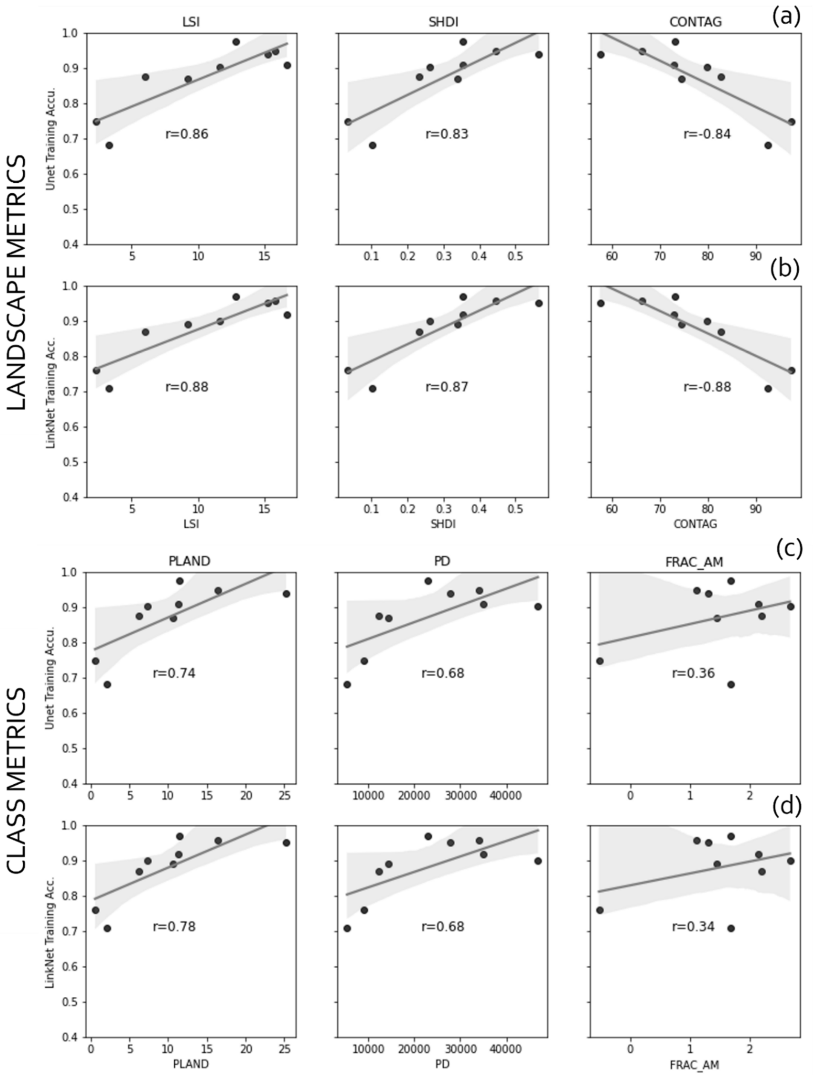
Analyze the relationship between spatial morphology of purple loosestrife patches and model performance;

(iii)

Explore repeat implementation strategies to evaluate model reusability.

This study used field-validated UAV imagery of two wetlands along the upper Mississippi River, situated in La Crosse County, Wisconsin, as a case study.

2. Vegetation Specie Mapping and Deep Learning Models

In the field of remote sensing, convolutional neural networks (CNN)-based DL models are revolutionizing vegetation mapping and specie identification [16,22]. The main advantage of these supervised deep CNN models is that they can take raw input data and autonomously learn relevant features during the training process using labeled masks of the target objects. Along with learned features, these models extract the contextual information of the object (e.g., overall structure of the plant or traits of the flowers) that are important for assigning the observations to the specified categories. The current DL techniques are establishing new avenues for object detection and pattern recognition. These techniques, along with use of very high-resolution UAV imagery, have the potential to radically change the way land surveys are performed. They offer the possibility to replace time-consuming (and sometimes dangerous) and labor-intensive field surveys and deploy AIP detection and monitoring system at a larger scale and with reduced cost [15,19].

Use of DL techniques using very high-resolution image segmentation and classification is still at an early stage. Within that field of literature, only a few studies have implemented such an approach to detect and map invasive plant species [22,23,24,25]. So far, different types of CNN models have been used for plant invasive species detection. One such model is SegNet, an encoder–decoder-cascaded CNN that was used with aerial multispectral images to demonstrate the potential of DL techniques to detect weeds in agricultural land [23]. Another study used a deep CNN model and compared it with other popular machine learning models to detect invasive hydrangea in the Brazilian national forest [24]. The DL model outperformed the other machine learning models with an accuracy of 99.71%. Specifically for detection of AIPs in wetlands, the CNN-U-Net model has been used to successfully identify blueberry bushes in a German wetland [22], and a combination of SegNet architecture and the ResNet50 encoder detected different vegetation communities in Irish wetlands with more than 90% accuracy [26]. Previous efforts by the present authors’ research team to detect purple loosestrife using semi-automated techniques such as object-based image classification with the random forest model and pixel-based classification using the VGG-16 CNN model resulted in 58% accuracy and 81% accuracy (F1 score), respectively. Although VGG-16 was a good approach for a very small spatial extent, the model failed to differentiate between other herbaceous plants for larger datasets and different study sites. Therefore, a more complex model was necessary to identify purple loosestrife patches. One of the most successful and popular fully connected CNN architectures is the U-Net model [27]. U-Net has been shown to outperform all traditional classification methods and has great potential for vegetation mapping [24,28]. Therefore, this study used U-Net architecture with a ResNet-152 encoder to map purple loosestrife from the UAV imagery. Further, the study compared the U-Net model with another popular architecture called LinkNet [29]. The LinkNet model is structurally similar to U-Net with a small difference of information transfer within the model. It has proven to be equally effective in capturing objects but with lesser run time.

3. Transfer Learning

Application of any deep CNN needs careful development of the training dataset and model training. A single model can have thousands of internal parameters; therefore, training a new model is computationally expensive and time-consuming [30]. By nature, the deep learning models learn from examples [31,32]. Therefore, domain experts have been using a technique called ‘transfer learning’, which allows for using an optimized pre-built model as the starting point to solve a new problem using less data [33]. These pre-built models only need to be fine-tuned to the new problem and thus saves the time required to train a model from scratch [34,35]. Transfer learning is crucial when repeat implementation is necessary [31]. For example, this study aims to produce a map that accurately detects purple loosestrife to aid eradication efforts. However, the classified map developed using a DL model and labeled data is only true for the time when the label data were collected and therefore not useful for consecutive years. In addition to developing and training models that are best suited for detecting any vegetation specie, development of labeled data is also one of the most time-consuming tasks. In this scenario, adopting a transfer learning approach to utilize a pre-trained model saves time and resources and can be implemented for areas where there is lack of labeled data. Therefore, transfer learning approach has been instrumental in making deep learning accessible to non-expert users [35].

For implementation of transfer learning, the users need to decide the ‘what’, ‘when’, and ‘how’ of knowledge transfer before they can accomplish the given task [31]. The ‘what’ corresponds to the knowledge that can be transferred across domains. A CNN structure has two parts, the first part is the convolutional base, which includes multiple convolution layers, activation functions, and pooling layers, and extracts generalized features from the input data. The second part is the classifier which includes fully connected layers and activation functions and learns about the specific features in the dataset and uses the information to classify the image [36]. The ‘when’ corresponds to the specific situation when transfer of knowledge results in efficient modeling. To conduct an efficient knowledge transfer, the source domain of the pre-trained model should be related to the target domain; otherwise, it can hurt the modeling approach [31]. Finally, the ‘how’ of knowledge transfer corresponds to the different approaches to successfully accomplish this task. Currently, there are three approaches to accomplish the transfer learning task, first is to use a model’s pre-built architecture and train the model from scratch with a large amount of labeled data from target domain. The second approach is to partially freeze the convolutional base and train the rest of the layers. The number of layers to freeze versus train depends on the amount of target dataset and number of parameters involved. Finally, the third approach is completely freezing the convolutional base, so the knowledge of the pre-trained model is kept intact and then the model is trained with the target dataset. This study experiments with the first and the third approaches of transfer learning, hereby named as ‘Experiment # 1′ and ‘Experiment # 2′, respectively. The detailed description of ‘Experiment # 1′ and ‘Experiment # 2′ are provided in the Data and Methodology, Section 4.5 and Section 4.6, respectively.

4. Data and Methodology

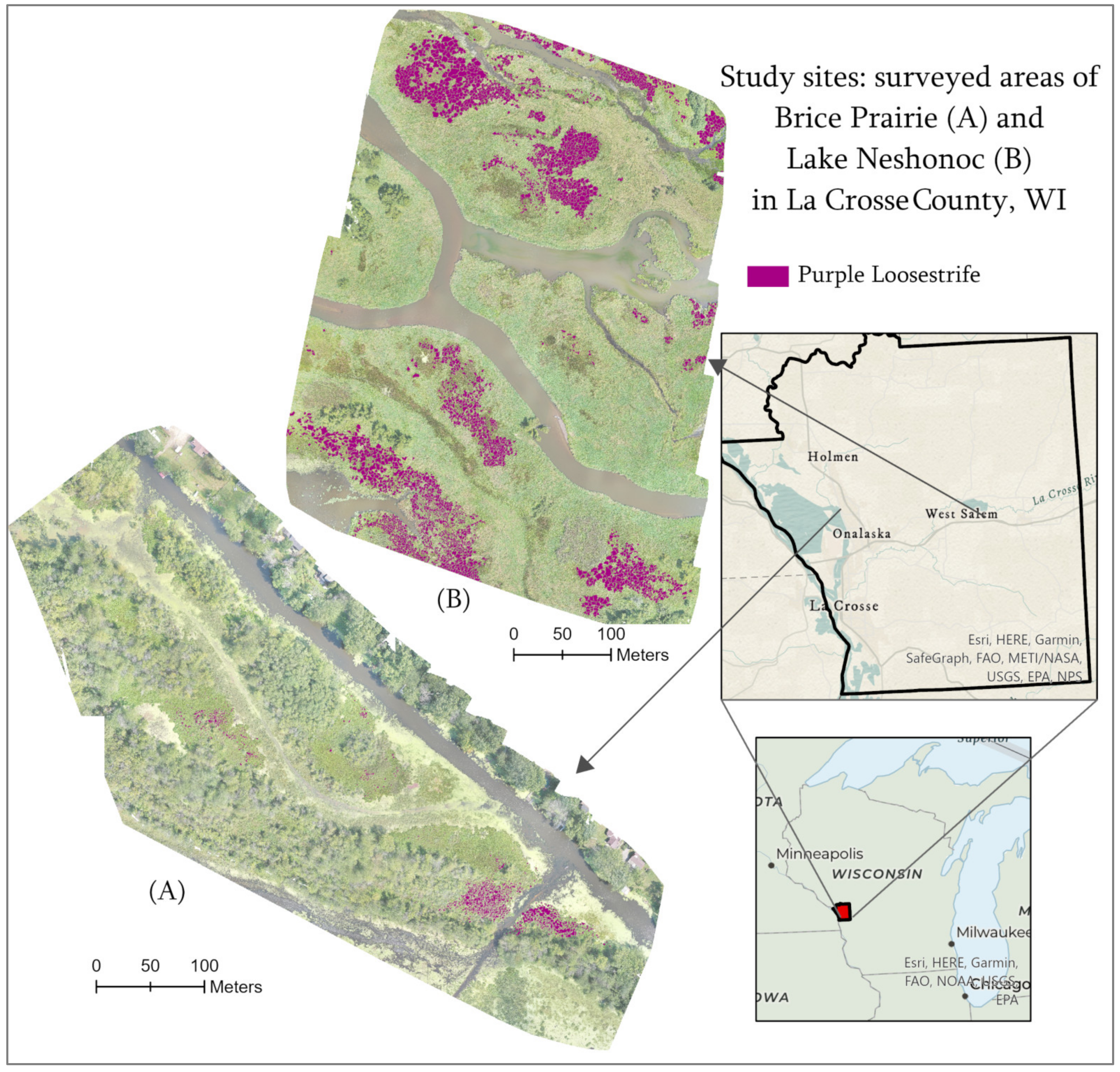
4.1. Study Area

UAV and ground data were acquired at two strategically selected locations (considering their physical accessibility and spatial distribution of purple loosestrife) within La Crosse County, Wisconsin. The Brice Prairie study site is located adjacent to the east banks of the Mississippi River and falls within the Upper Mississippi National Wildlife and Fish Refuge (Figure 1A). A local conservation organization (i.e., Brice Prairie Conservation Association) has been actively applying biocontrol to eradicate purple loosestrife at this location. The biocontrol measures have had limited success due to influx of flood waters from the lock and dam system on the Mississippi River’s Pool 8. The second study site is located on the La Crosse River delta (Figure 1B) and is directly upstream from Lake Neshonoc. This wetland was created by damming the La Crosse River and lies about 20 km east of the Brice Prairie site (Figure 1).

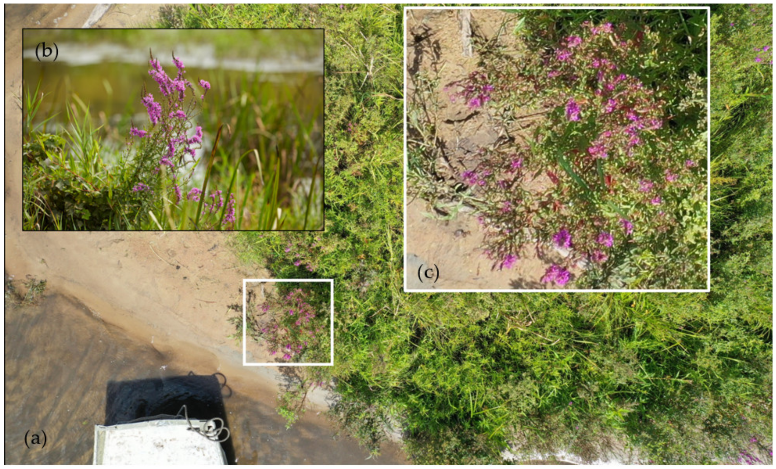
4.2. UAV Data Acquisition and Post-Processing

One of the challenges in identifying purple loosestrife is the similarity of the plant structure with the surrounding vegetation in its habitat. In the existing literature of invasive species identification using UAV imagery and DL models [15,22,26], the target species were distinctly identifiable from the images due to its bare earth background, structure of the target, or low-density growth. Purple loosestrife, on the other hand, is impossible to identify during non-flowering season due to its resemblance with the surrounding native grass. During the flowering season the only distinctive identifying feature is its purple-colored flowering stalk [37]. Therefore, late July–early August, which is the flowering peak, is the most suitable time for mapping purple loosestrife. For this study, UAV imagery was acquired for the Brice Prairie site on 31 July 2019, while the La Crosse River delta site was mapped on 6 August 2019. The weather on these days represented clear sunny skies with calm/no winds. For both study sites, images were acquired by a rotary-wing UAV (Mavic 2 Pro from DJI 2019) fitted with a GNSS satellite positioning system and a 20 mega-pixel Hasselblad camera (i.e., 5472 by 3648 pixels) that captures JPEG images. The Map Pilot app (2017) for DJI was used to pre-program mission parameters. These parameters were used with autopilot to capture images in a grid pattern at a constant elevation (with respect to ground) using the ‘terrain follow’ feature. Image acquisition constituted 3 flights at the Brice Prairie site and 4 flights at the Lake Neshonoc site. For all flights, the average flight altitude was 60 m above ground, with forward image overlaps of 80%, side overlap of 75%, and flight speed of 3 m s⁻¹. Owing to the wetland setting of the area, it was not possible to establish any temporary or permanent ground control points. The collected images were processed following standard structure-from-motion (SfM) workflows in the Pix4Dmapper Pro software. Specific details of the algorithms implemented in the Pix4D package are not available due to the proprietary nature of the software, but some details regarding the parameters utilized within the software can be found in Pix4D documentation (2019). The SfM processing yielded orthomosaics (0.02 m spatial resolution) that were corrected for perspective error using a digital surface model for each study site (Figure 2).

4.3. Image Data and Reference Data Preparation

The reference data referred to as ‘masks’ were developed by visual interpretation and manual delineation of the purple loosestrife from the orthomosaics. Each image mosaic was carefully evaluated, and purple loosestrife patches were labeled. This process of semantic labeling of pixels in imagery is of paramount importance [38] and is the most time-consuming and labor-intensive part of the supervised image classification approach. The manually digitized masks were cross-checked and validated with field data to maintain high accuracy. Both study sites (Brice Prairie = 35 ha, and Lake Neshonoc = 22.39 ha) were subdivided into smaller image subsets, which were around 10% of the whole image of a study site, where there was a high level of invasion (Figure 3). These subsets were created with dual purpose, first, to restrict time and modeling resources to accurately identify purple loosestrife only; and second, to evaluate the effect of spatial morphology of the purple loosestrife patches on model performance, which will be useful for future applications in other areas. All image subsets were subjected to the same data preparation pipeline, where first image masks were prepared with the labeled data, then the RGB imagery and the masks were split into smaller tiles called chips for model training and prediction.

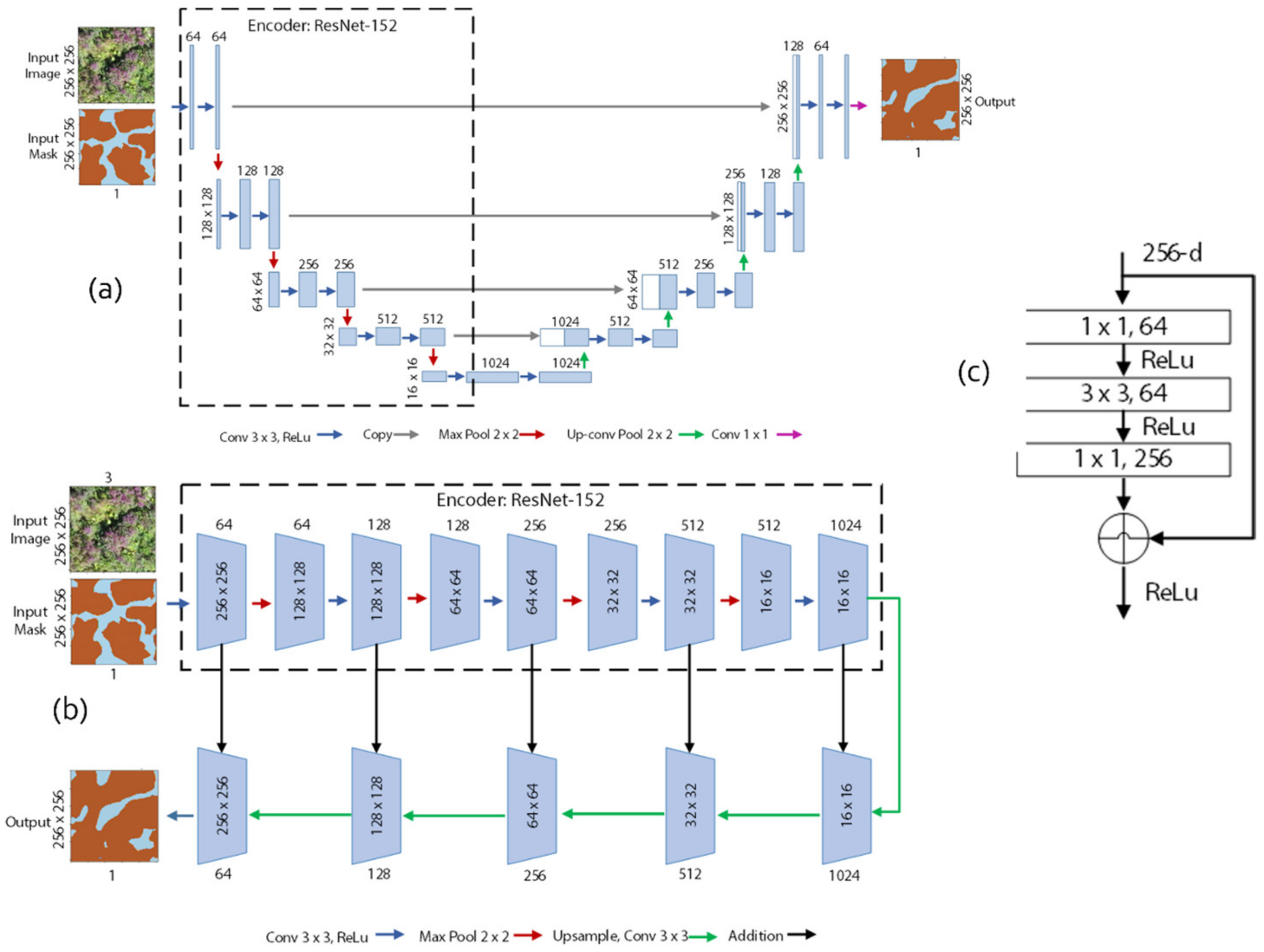
4.4. U-Net and LinkNet Models

This study used the U-Net (Figure 4a) and the LinkNet model (Figure 4b) with ResNet-152 as the encoder (Figure 4c). The U-Net architecture is composed of an encoder or downsampling path and a decoder or upsampling path. The encoder extracts the most relevant features from the input layers and reduces the size of the images. As the model goes through downsampling, it stores the information regarding image transformation in form of weights of matrices along every step. The decoder uses the information from the encoder to perform segmentation and to upsample the output back to its original full size. The LinkNet model [29] has similar architecture as U-Net with a small difference. In addition to going through a step-by-step downsampling task, LinkNet transfers the spatial information directly from the encoder to the corresponding decoder. By directly transferring the spatial information from the encoder to the decoder, it recovers the spatial information from the step-by-step process which otherwise would have been lost. Therefore, the overall accuracy of the classification task improves. Additionally, owing to the transfer of knowledge from encoder to decoder at every layer, the decoder can use fewer parameters to run the segmentation task, which results in reduced training time. In this study, both models used ResNet-152 [39] as backbone or encoder, which means the ResNet-152 model was used to extract features to build the segmentation model. During the downsampling process, when the model is going through creating weighted layers, the ResNet models add a residual map after every few encoding blocks of 3 × 3 convolutional layer. In the ResNet-152 model, an extra 1 × 1 convolutional layer is added before and after the 3 × 3 convolutional layer, called a ‘bottleneck’ building block (Figure 4c) that creates a deeper network and significantly reduces the problem of vanishing gradient [39].

As mentioned previously in Section 3, out of the three existing approaches of transfer learning, this study adopted the first and the third approach. In the first approach, named ‘Experiment # 1′, the U-Net and the LinkNet models were used (Figure 3) to train the purple loosestrife dataset for each subset individually. In the second approach, named as ‘Experiment # 2′, all image subsets of Lake Neshonoc were trained and tested together (hereby named ‘Lake Neshonoc model’). The Lake Neshonoc model was the retrained with one of the subsets from Brice Prairie dataset (BP 1) with frozen layers and tested for accuracy. More details on the model training in Experiment # 1 and Experiment # 2 are provided in the Section 4.5 and Section 4.6 below, respectively.

4.5. Experiment # 1

Based on the knowledge gained from existing literature, in Experiment # 1, both the U-Net and the LinkNet models were iteratively evaluated and fine-tuned using the following variations in hyper-parameter to find the most optimum set: batch size (8, 12, 24, 32, 64), epochs (50, 100, 500, 1000), learning rate (0.001, 0.0001), tile size ({128, 128}, {256, 256}, {512, 512}), activation functions (sigmoid, ReLu), and encoder weights (ImageNet, random). Each subset was also tested using two variations in input image, first the model training and testing was done with only RGB imagery and secondly, the RGB imagery was stacked with an additional enhanced bloom index (EBI) layer, which measures floral phenology by enhancing the bloom’s spectral signature while weakening the background spectral signals from surrounding vegetation and soils [40]. The 9 image subsets (7 subsets from Lake Neshonoc and 2 subsets from Brice Prairie) were trained and tested individually. The U-Net and the LinkNet architectures were unchanged, and the models were trained from scratch for each image subset for which 75% of the data were used for training and 25% for testing. The code was written in Python using the Keras [41] with the TensorFlow backend v.2.0.0 [42] and Segmentation model package [43]. The model training was done using NVIDIA GeForce RTX 3090 GPU.

4.6. Experiment # 2

The goal of Experiment # 2 was to develop a reusable model for repeat implementation in the future. For this study, a model was defined as reusable if it satisfies two conditions: first, its training time with a new dataset should be less than training the model from scratch, and second, its training accuracy should be same or higher than the accuracy achieved by training from scratch. In Experiment # 2 (Figure 5), all image subsets (8711 chips) of the Lake Neshonoc site were merged and trained together using the U-Net and the LinkNet model with the ResNet-152 encoder. The set of hyper-parameters that resulted in the highest accuracy in Experiment # 1 were used here with a 75–25 split between training and testing images. For implementation, the convolutional base of each of the Lake Neshonoc models was frozen and then the model was trained with BP1 dataset with relatively smaller amount of labeled data compared to its corresponding model training from scratch in Experiment # 1. Given the context that the source data in the Lake Neshonoc model and the target data in BP1 were the same species, the theoretical assumption was that the features learned from the images of Lake Neshonoc site would be used for segmentation and classification in BP1 subset and should result in an acceptable level of training accuracy. The models were run for 20, 40, 60, 80, and 100 epochs to test the minimum number of epochs needed to match or exceed the accuracy achieved during the BP1 subset’s model training from scratch.

4.7. Accuracy Assessment

In this study, mean intersection-over-union (IoU) and F1-score are popular evaluation metrics for image segmentation with binary classification and both were computed to assess the training and validation accuracy. IoU, also known as the Jaccard index, is extensively used in object detection. IoU is calculated by dividing the area of overlap between the predicted segmentation of the target object and its corresponding ground-truth mask by the area of union between the predicted segmentation and the ground mask. For multi-class segmentation, IoU is computed for each class and then it returns the mean of IoUs for the image. In other words, the IoU metric for individual class can be defined as:

$$IoU=\frac{TP}{\left(TP+FP+FN\right)}$$

(1)

where, TP = true positive, FP = false positive, and FN = false negative [24]. Further, the study also used F1-score, which has been popularly applied to semantic segmentation in UAV imagery. F1-score, also known as the Dice coefficient, is the harmonic mean of precision and recall. In other words, F1-score can be defined as:

$$F1=\frac{2\times \left(\mathit{Precision}\times \mathit{Recall}\right)}{\left(\mathit{Precision}+\mathit{Recall}\right)}$$

(2)

where,

$$\mathit{Precision}=\frac{TP}{\left(TP+FP\right)}$$

(3)

$$\mathit{Recall}=\frac{TP}{\left(TP+FN\right)}$$

(4)

Both IoU and F1-score are positively correlated, which means that if one metric infers that model 1 is better than model 2, then the other metric will infer the same. However, IoU scores are more conservative than F1-scores because IoU scores are closer to the minimum of precision and recall, whereas the F1-scores are closer to the average of precision and recall across all images. In this study, the results are discussed using the mean IoU values.

4.8. Patch Morphology with Spatial Metrics

The study used spatial metrics [44] to measure the level of fragmentation in each image subset and evaluate the relationship between fragmentation level and model accuracy. At the landscape level, this study used landscape shape index (LSI), Shannon’s diversity index (SHDI), and contagion index (CONTAG). LSI and CONTAG are measures of aggregation, and SHDI is a measure of diversity in the landscape. Higher LSI values indicate more irregular shape of the patches. Higher CONTAG values indicate landscapes with a few large, contiguous patches and low values indicate smaller and more disaggregated patches [45]. Similarly, SHDI value of a landscape increases as the proportional distribution of area among patch types becomes more equitable. At class level, proportion of land (PLAND), patch density (PD), and area mean fractal dimension (FRAC_AM) were measured. PLAND and PD measures the relative abundance of specific class-level patch in the landscape, whereas higher FRAC_AM values indicate that the patches are large and highly convoluted [44].

5. Results

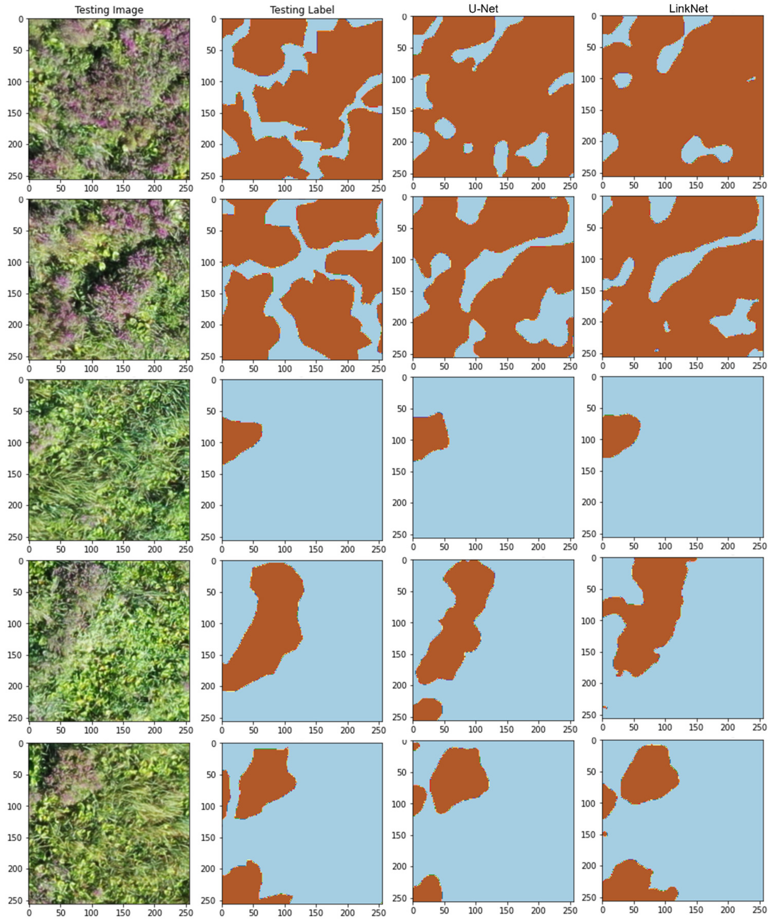
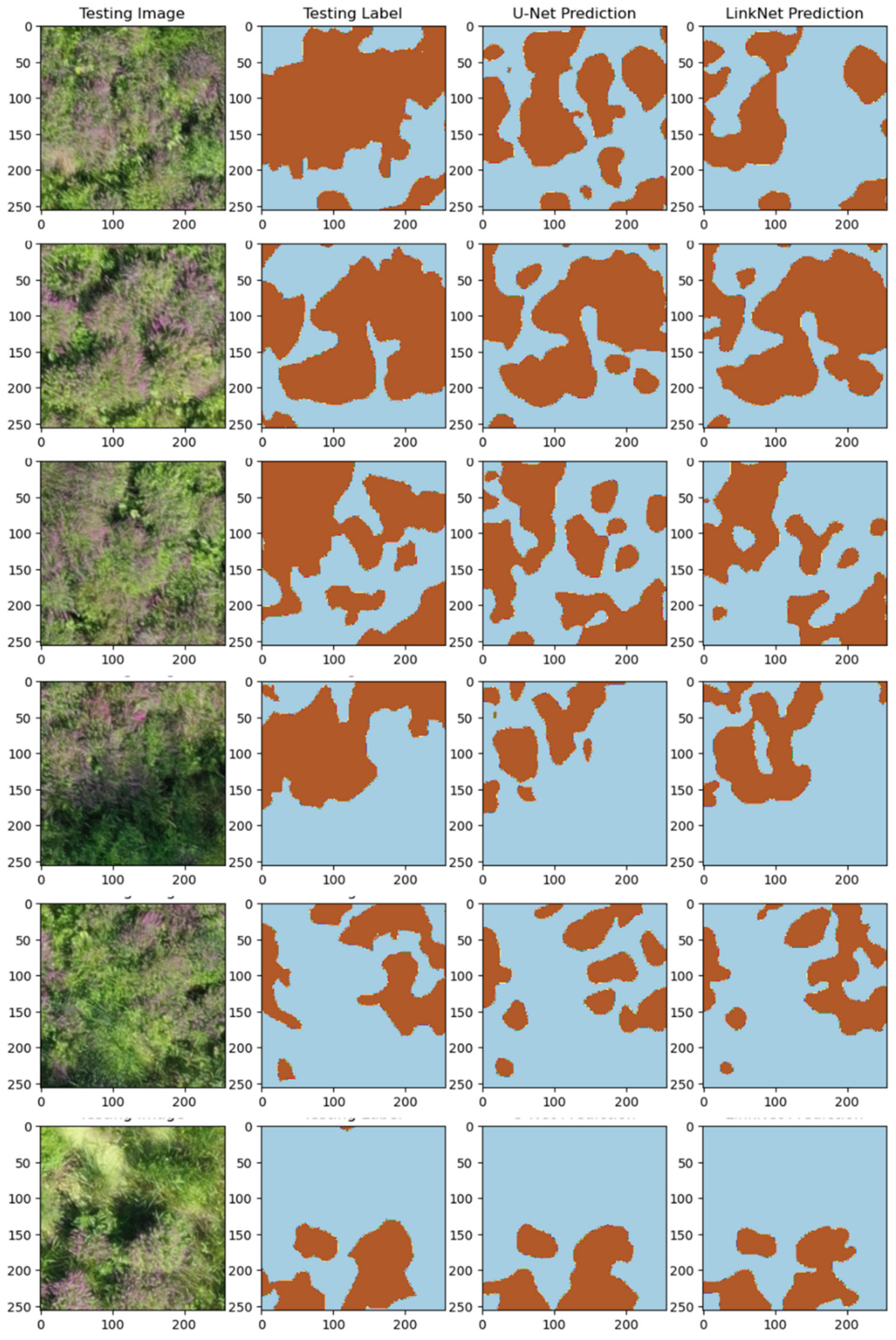
5.1. Model Training and Testing—Experiment # 1

After iterative evaluation of both the models with different combination of hyper-parameters, the best set of results were generated by using the tile size 256 × 256, with batch size 12, 100 epochs, learning rate of 0.0001, sigmoid activation function, and initialization with ImageNet weights. The best result in this study was defined as the set of parameters that generated the highest training and testing accuracy and completed in the least amount of time. The image tile size 128 × 128 was too small to capture even medium-sized patches, whereas 512 × 512 was too large and resulted in a higher number of false positives, mostly due to dried prairie grasses surrounding the purple loosestrife patches. The accuracy generated by the batch size of 8 was relatively lower than batch size 12; however, the model run was faster. With bigger batch sizes, the training accuracy levels were similar, but each epoch run and therefore the whole model run took longer. The models were run with a callback for ‘earlystopping patience’, which monitored training loss and was programmed to stop if the training loss did not change for 25 consecutive epochs. This approach helped to identify the ideal number of epochs for each run and in most cases achieved good results within 100 epochs. Since this study aimed to generate a binary map with presence and absence of purple loosestrife, the sigmoid activation function proved to be more appropriate for the task. The model runs with additional EBI layer generated around 0.5–4% higher accuracy than its corresponding model run with just RGB layers. However, the model run time was longer and the overall effort to prepare and process data resulted in a longer modeling task. So, it was a tradeoff between small and inconsistent increase in training accuracy versus a longer modeling task. Among all the hyper-parameters, model initialization with ImageNet weights was the most significant one to improve both training and testing accuracy and run time.

Table 1. Results from Experiment # 1 showing training and testing accuracy using both mean IoU and F1-score for U-Net and LinkNet models for each image subset.

Img	Training				Testing
	IoU		F1-Score		IoU		F1-Score
	U-Net	LinkNet	U-Net	LinkNet	U-Net	LinkNet	U-Net	LinkNet
LK0	0.88	0.87	0.90	0.89	0.63	0.55	0.63	0.60
LK1	0.94	0.95	0.96	0.96	0.68	0.68	0.80	0.80
LK2	0.98	0.97	0.99	0.98	0.73	0.72	0.82	0.81
LK3	0.87	0.89	0.90	0.91	0.54	0.57	0.66	0.72
LK4	0.68	0.71	0.67	0.69	0.65	0.62	0.68	0.75
LK5	0.91	0.92	0.94	0.95	0.55	0.54	0.59	0.58
LK6	0.95	0.96	0.95	0.95	0.66	0.71	0.77	0.73
BP1	0.90	0.90	0.90	0.91	0.68	0.70	0.74	0.75
BP2	0.75	0.76	0.78	0.76	0.50	0.50	0.50	0.50

shows the mean IoU values and F1-scores of both the U-Net and LinkNet models with the ResNet-152 encoder with optimal hyper-parameters. Overall, the training accuracy of the LinkNet model was similar or better than the U-Net model, whereas its testing accuracy was similar or worse than the U-Net model, which suggests that the U-Net model’s feature knowledge was more generalizable than LinkNet’s. Relatively higher testing accuracy in U-Net could be attributed to a larger number of trainable parameters than the LinkNet model, which led to longer run time (

Table 2. The number of chips, total land area in hectares (ha), and proportion of area covered by the purple loosestrife class in each image subset. The number of chips (# chips) in the table refers to the number of tiles each image subset was split into based on 256 × 256 tile size.

Img	Time (mm.ss)		Chips #	Total Area (ha)	Class Area (%)
	U-Net	LinkNet
LK0	26:09	23:15	1040	1.81	6.20
LK1	24:27	22:27	930	1.60	25.22
LK2	39:35	36:47	1550	2.67	11.41
LK3	27:38	27:03	1092	1.88	10.68
LK4	32:32	30:03	1274	2.16	2.07
LK5	39:31	36:39	1550	2.64	11.36
LK6	32:29	30:11	1275	2.16	16.41
BP1	37:57	35:09	1476	1.48	7.30
BP2	20:44	23:58	1023	1.04	0.57

). As a result, the LinkNet model was consistently faster in almost in subset applications (Table 2). Although there is no consistent relationship between proportion of the landscape occupied by the purple loosestrife patches and model accuracies, in LK 4 and BP2, where the purple loosestrife patches only covered around 0.6–2% of the landscape, the model accuracies were lower. The model run time was also correlated to the number of image chips used in each model run, which means the subsets with larger number of chips took longer to complete than the ones with smaller number of chips. It is intuitive to believe that a larger number of chips mean a bigger area covered by the input image, but that was not true for all input image subsets. If an image was a perfect square, then the number of chips corresponds to the total area covered by the image. However, if the image was not a square, then the nearest rectangular bounding box of NoData was generated to create square image chips. Therefore, an input image with small spatial extent but geometrically irregular shape could result in a large number of NoData chips during the pre-processing stage.

Figure 6 shows a few selected predicted images from the U-Net and LinkNet models. Visually, the predicted images from both the models were very similar to the ground-truth mask (testing label). However, close comparison between the predicted images and the ground-truth mask shows that the patches in the LinkNet-predicted images were more generalized and smoother than the U-Net-predicted images.

5.2. Spatial Metrics

Different landscape-level and class-level spatial metrics were used to understand the relationship between spatial morphology of the landscape and model accuracies. Figure 7 shows the relationship between spatial metrics and training accuracy of the U-Net and LinkNet models for each image subset. At landscape level (Figure 7a,b), there was strong positive correlation between the training accuracies and the LSI and the SHDI values, which suggested that the model performed better when the landscape contained more irregularly shaped equitably distributed patches. There was a strong negative correlation between the training accuracies and CONTAG values, which suggested that the model performed better in landscapes with smaller and disaggregated patches. The strength of relationship was comparatively stronger between the training accuracies of the LinkNet model and the landscape-level metrics, which suggested that spatial morphology of the patches was relatively more influential in the LinkNet model than the U-Net model. At class level (Figure 7c,d), PLAND and PD had positive correlation with training accuracies, which suggested that model performed better in images with relatively higher abundance of purple loosestrife patches. The strength of correlation between FRAC_AM and training accuracies was relatively weaker than other metrics, which suggested that patch complexity and model performance had a weak relationship. The study did not investigate the relationship between testing accuracy and spatial metrics; however, the results showed that image subsets with lower PD and LSI values (LK0, LK3, LK4, BP2) had relatively lower testing accuracies. Overall, the strength of relationship between models’ training accuracy and landscape-level metrics was relatively stronger than the class-level metrics.

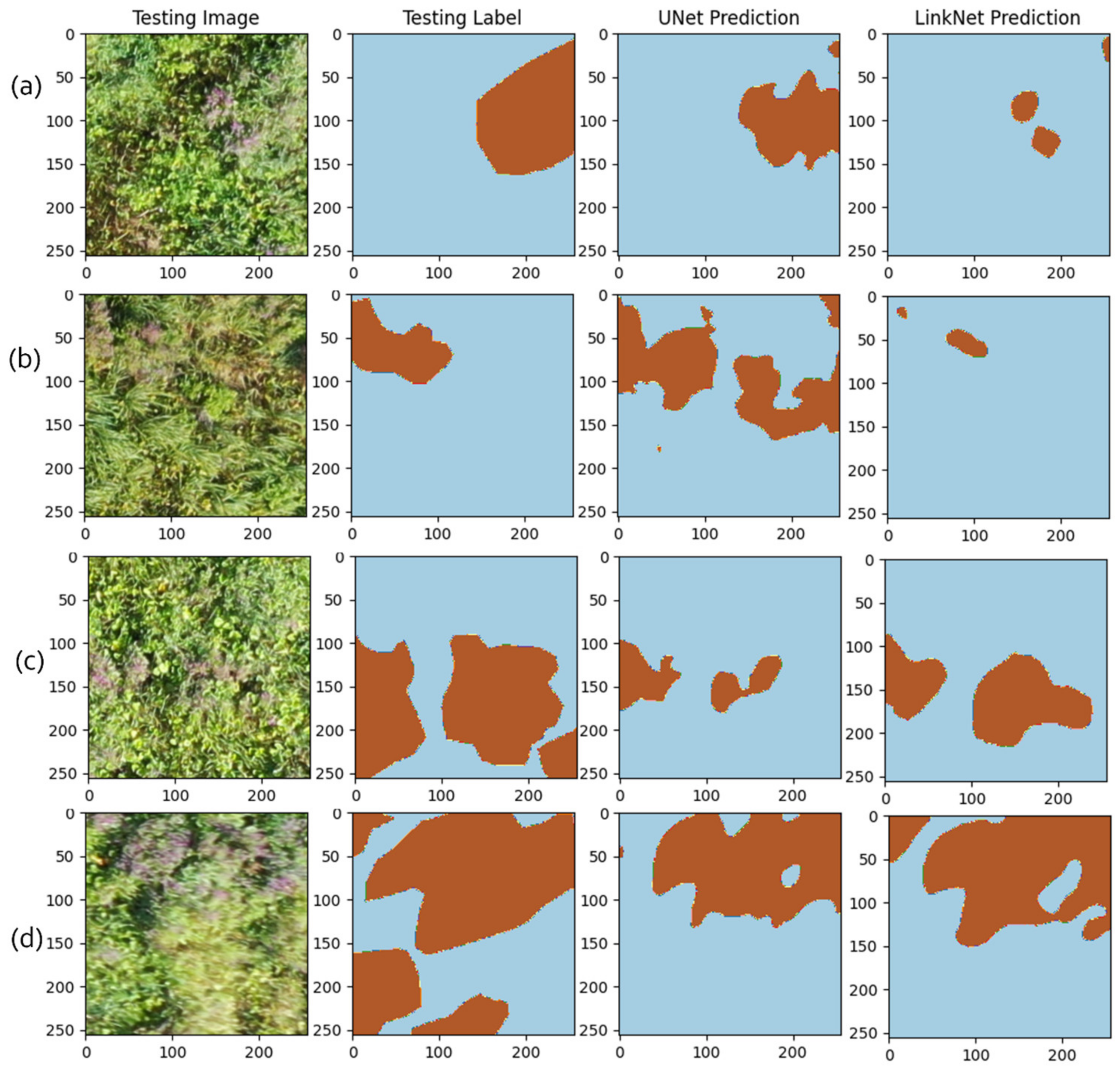
5.3. Model Training and Testing—Experiment # 2

In Experiment # 2, the study used the best-performing hyper-parameters combination in Experiment # 1 (tile size of 256 × 256, initialization with ImageNet weights, sigmoid activation function, learning rate of 0.0001, batch size 12, and 100 epochs). The results from Experiment # 2 showed that the Lake Neshonoc model, which consisted of all the images of Lake Neshonoc subsets (8711 images), generated a training accuracy (mean IoU) of 0.86 (F1-score = 0.90), 0.87 (F1-score = 0.91) and testing accuracy (mean IoU) of 0.62 (F1-score = 0.75), 0.62 (F1-score = 0.75) using the U-Net and LinkNet models, respectively, and the LinkNet model was 15 min faster for the 100 epochs run than the U-Net model (

Table 3. Experiment # 2 results showing the training and testing accuracy (both mean IoU and F1-score) and the time taken by the Lake Neshonoc models and the Brice Prairie subsets with different epoch runs.

Img	Epochs	Training				Testing				Time (h:mm:ss)
		IoU		F1-Score		IoU		F1-Score
		U-Net	LinkNet	U-Net	LinkNet	U-Net	LinkNet	U-Net	LinkNet	U-Net	LinkNet
LK	100	0.86	0.87	0.90	0.91	0.62	0.62	0.75	0.75	3:40:07	3:25:15
BP1	20	0.89	0.89	0.93	0.98	0.72	0.70	0.81	0.84	0:07:45	0:07:55
	40	0.93	0.91	0.95	0.96	0.70	0.70	0.80	0.85	0:15:08	0:15:12
	60	0.95	0.91	0.96	0.98	0.70	0.83	0.86	0.82	0:22:40	0:22:51
	80	0.86	0.93	0.93	0.94	0.73	0.81	0.89	0.78	0:30:13	0:30:20
	100	0.90	0.83	0.96	0.96	0.79	0.71	0.85	0.76	0:37:39	0:37:55

) using NVIDIA GeForce RTX 3090 GPU. Both the models were then subsequently used for the Brice Prairie site and re-trained with BP1 subset data (1476 images). The results (Table 3) show that both U-Net and LinkNet models were able to achieve training mean IoU of 0.89 (F1-score: 0.90–0.91) and testing mean IoU of 0.70–0.72 (F1-score: 0.80–0.85) in 20 epochs within 8 min. The training mean IoU of 0.91–0.93 (F1-score: 0.95–0.96) and testing mean IoU of 0.70–0.72 (F1-score: 0.80–0.85) was achieved in 40 epochs in around 15 min (Table 3). These training and testing accuracy values were higher than the model run from scratch in Experiment # 1 (Table 1) and were achieved in less than half its time (Table 2). However, the training accuracies decreased with 80 and 100 epochs, which suggested that the model over-fitted and was therefore unable to accurately predict the patches. The models were run again with 80 and 100 epochs with a lower learning rate (0.00001), which resulted in relatively higher accuracy but longer training time than its corresponding 80 and 100 epoch runs with a learning rate of 0.0001. Contrary to the model runs from the scratch in Experiment # 1, in Experiment # 2 the U-Net Lake Neshonoc model implementation with the BP 1 dataset resulted in relatively higher accuracy and faster run time. The U-Net and LinkNet model runs with 40 epochs were used to generate predicted images to evaluate the pattern of the predicted patches (Figure 8). The images show that both U-Net and LinkNet models predicted similar patch patterns. Both models were able to generate more disaggregate patches even when the labeled masks represented a more generalized and aggregated patch outline. In some cases, the U-Net model was able to capture smaller patches better than the LinkNet model. Overall, within the context of repeat implementation, the U-Net Lake Neshonoc model performance in terms of speed and training accuracy was better, which may be attributed to the larger number of trainable parameters, resulting in more generalizable results.

6. Discussion

The objectives of this study were to evaluate a deep learning methodology to correctly identify purple loosestrife patches, to understand whether spatial morphology of patches influence model performance, and finally, to find an approach that can be repeatedly implemented in different study areas to continuously map and monitor purple loosestrife outbreaks. The study demonstrated that although the training accuracies of the LinkNet model were better and the model runs were consistently faster in Experiment # 1, the U-Net model generated similar or better testing accuracies. Better testing accuracies suggested that features learned by the U-Net model during training were more generalizable and therefore better for repeat implementation with a new dataset. The analysis of the relationship between spatial metrics and the training accuracies showed that both the models performed better in image subsets where the landscape was occupied by smaller, equitably distributed, and disaggregated purple loosestrife patches. LinkNet model accuracies had a relatively stronger relationship with the landscape-level metrics than that of the U-Net model. Further, in Experiment # 2, the study demonstrated that for repeat implementation, the U-Net model outperformed the LinkNet model in speed and in training and testing accuracies. The model run for the Brice Prairie image subset (BP1) in Experiment # 2 was much faster and more accurate than the model run from scratch in Experiment # 1, which resulted in less computer resource consumption.

The predicted images generated in both Experiment # 1 and Experiment # 2 showed that both models were able to successfully detect and identify the purple loosestrife patches in the imagery. In fact, in some cases (Figure 9a–c), where the labeled patches were over-generalized or aggregated due to error in human judgment during the digitization process, the models were able to identify the smaller patches distinctively in the imagery. During the labeled mask data development process, the goal was to only create masks (polygons) around the flowering stalks because individual bushes were circular, and the stalks were dense and well distributed within it. However, during digitation of purple loosestrife patches, in some cases it was difficult to determine the patch boundary clearly. For instance, when two individual bushes were not close enough to be part of a single patch, but not far enough apart to be considered as a distinctly separate single patch, then the decision to draw the outlines was subject to human interpretation and therefore over-generalized. This mismatch was one of the reasons for some of the lower accuracies due to inaccurate segment-to-segment match. However, when the predicted images were visually compared to the original image, it was found that both LinkNet (Figure 9a,b) and U-Net (Figure 9c) successfully identified just the flowering stalk part. However, the U-Net model specifically over-predicted where there was dried prairie grass around the flowering stalk. The models were also able to identify purple loosestrife patches from the images that were blurred due to orthorectification (Figure 9d).

Despite deep CNN’s superlative performance in various types of land cover and vegetation mapping, one of the biggest reasons for their sparse application is the need for ample reference data for model training. Among all existing supervised machine learning classifiers, deep CNN models require the largest amount of reference observations for identifying and learning the image and its contextual features [15,26]. However, owing to deep CNN’s transfer learning capability [46], there is a rising effort to create land cover or vegetation-specific reference database repositories [47]. Therefore, the Lake Neshonoc models developed in Experiment # 2, along with the training data will be highly beneficial for future studies in purple loosestrife identification. The model and the dataset will be hosted via the authors’ GitHub platform and will be shared with local natural resource managers.

7. Conclusions

The purple loosestrife detection methodology demonstrated in this study provides a state-of-the-art solution for local and regional environmental managers to map and monitor new invasions efficiently. Not only it has the potential to map known spatial extent of the invasion, but also it can detect purple loosestrife in areas where its existence was not explored due to inaccessibility of the area or a need to preserve critical habitat that could be disturbed by field-based sampling. Repeat implementation of a pre-trained model with a new dataset will be useful for identifying new invasion locations more efficiently, and therefore will be beneficial for continuous monitoring and strategic planning in the application of direct biocontrol measures.

References

1. Prentis, P.J.; Wilson, J.R.U.; Dormontt, E.E.; Richardson, D.M.; Lowe, A.J. Adaptive Evolution in Invasive Species. Trends Plant Sci. 2008, 13, 288–294. [Google Scholar] [CrossRef] [PubMed]
2. Early, R.; Bradley, B.A.; Dukes, J.S.; Lawler, J.J.; Olden, J.D.; Blumenthal, D.M.; Gonzalez, P.; Grosholz, E.D.; Ibañez, I.; Miller, L.P.; et al. Global Threats from Invasive Alien Species in the Twenty-First Century and National Response Capacities. Nat. Commun. 2016, 7, 16. [Google Scholar] [CrossRef] [PubMed] [Green Version]
3. Havel, J.E.; Kovalenko, K.E.; Thomaz, S.M.; Amalfitano, S.; Kats, L.B. Aquatic Invasive Species: Challenges for the Future. Hydrobiologia 2015, 750, 147–170. [Google Scholar] [CrossRef] [PubMed]
4. Pyšek, P.; Richardson, D.M. Invasive Species, Environmental Change and Management, and Health. Annu. Rev. Environ. Resour. 2010, 35, 25–55. [Google Scholar] [CrossRef] [Green Version]
5. Walsh, J.R.; Carpenter, S.R.; Van Der Zanden, M.J. Invasive Species Triggers a Massive Loss of Ecosystem Services through a Trophic Cascade. Proc. Natl. Acad. Sci. USA 2016, 113, 4081–4085. [Google Scholar] [CrossRef] [Green Version]
6. Olden, J.D.; Tamayo, M. Incentivizing the Public to Support Invasive Species Management: Eurasian Milfoil Reduces Lakefront Property Values. PLoS ONE 2014, 9, e110458. [Google Scholar] [CrossRef] [Green Version]
7. Johnson, M.; Meder, M.E. Effects of Aquatic Invasive Species on Home Prices. 2013. Available online: https://ssrn.com/abstract=2316911 (accessed on 29 November 2022).
8. Connelly, N.A.; Lauber, T.B.; Stedman, R.C.; Knuth, B.A. The Role of Anglers in Preventing the Spread of Aquatic Invasive Species in the Great Lakes Region. J. Great Lakes Res. 2016, 42, 703–707. [Google Scholar] [CrossRef] [Green Version]
9. Fantle-Lepczyk, J.E.; Haubrock, P.J.; Kramer, A.M.; Cuthbert, R.N.; Turbelin, A.J.; Crystal-Ornelas, R.; Diagne, C.; Courchamp, F. Economic Costs of Biological Invasions in the United States. Sci. Total Environ. 2022, 806, 151318. [Google Scholar] [CrossRef]
10. Bradshaw, C.J.A.; Leroy, B.; Bellard, C.; Roiz, D.; Albert, C.; Fournier, A.; Barbet-Massin, M.; Salles, J.M.; Simard, F.; Courchamp, F. Massive yet Grossly Underestimated Global Costs of Invasive Insects. Nat. Commun. 2016, 7, 12986. [Google Scholar] [CrossRef] [Green Version]
11. Bisbee, G.; Blumer, D.; Burbach, D.; Iverson, B.; Kemp, D.; Richter, L.; Sklavos, S.; Strohl, D.; Thompson, B.; Welch, R.J.; et al. Purple Loosestrife Biological Control Activities for Educators; Wisconsin Department of Natural Resources, Wisconsin Wetland Association: Madison, WI, USA, 2016; PUBL-SS-981 REV2016. [Google Scholar]
12. University of Wisconsin Sea Grant and Water resource Institute. Wisconsin Aquatic Invasive Species Management Plan; Wisconsin Department of Natural Resources: Madison, WI, USA, 2018. [Google Scholar]
13. Wisconsin DNR. Wisconsin Invasive Species Program Report; Wisconsin Department of Natural Resources: Madison, WI, USA, 2015. [Google Scholar]
14. US Dept of the Interior. Safeguarding America’s Lands and Waters from Invasive Species: A National Framework for Early Detection and Rapid Response Contents; US Dept of the Interior: Washington, DC, USA, 2016.
15. Kattenborn, T.; Eichel, J.; Fassnacht, F.E. Convolutional Neural Networks Enable Efficient, Accurate and Fine-Grained Segmentation of Plant Species and Communities from High-Resolution UAV Imagery. Sci. Rep. 2019, 9, 17656. [Google Scholar] [CrossRef] [Green Version]
16. Grenzdörffer, G.J.; Engel, A.; Teichert, B. The Photogrammetric Potential of Low-Cost Uavs in Forestry and Agriculture. Int. Arch. Photogramm. Remote Sens. Spat. Inf. Sci.-ISPRS Arch. 2008, 31, 1207–1214. [Google Scholar]
17. Raparelli, E.; Bajocco, S. A Bibliometric Analysis on the Use of Unmanned Aerial Vehicles in Agricultural and Forestry Studies. Int. J. Remote Sens. 2019, 40, 9070–9083. [Google Scholar] [CrossRef]
18. Tang, L.; Shao, G. Drone Remote Sensing for Forestry Research and Practices. J. Res. 2015, 26, 791–797. [Google Scholar] [CrossRef]
19. Kentsch, S.; Caceres, M.L.L.; Serrano, D.; Roure, F.; Diez, Y. Computer Vision and Deep Learning Techniques for the Analysis of Drone-Acquired Forest Images, a Transfer Learning Study. Remote Sens. 2020, 12, 1287. [Google Scholar] [CrossRef] [Green Version]
20. Gambella, F.; Sistu, L.; Piccirilli, D.; Corposanto, S.; Caria, M.; Arcangeletti, E.; Proto, A.R.; Chessa, G.; Pazzona, A. Forest and UAV: A Bibliometric Review. Contemp. Eng. Sci. 2016, 9, 1359–1370. [Google Scholar] [CrossRef]
21. Natesan, S.; Armenakis, C.; Vepakomma, U. Resnet-Based Tree Species Classification Using Uav Images. Int. Arch. Photogramm. Remote Sens. Spat. Inf. Sci.-ISPRS Arch. 2019, XLII-2/W13, 475–481. [Google Scholar] [CrossRef] [Green Version]
22. Cabezas, M.; Kentsch, S.; Tomhave, L.; Gross, J.; Larry, M.; Caceres, L.; Diez, Y. Remote Sensing Detection of Invasive Species in Wetlands: Practical DL with Heavily Imbalanced Data. Remote Sens. 2020, 12, 3431. [Google Scholar] [CrossRef]
23. Sa, I.; Chen, Z.; Popovic, M.; Khanna, R.; Liebisch, F.; Nieto, J.; Siegwart, R. WeedNet: Dense Semantic Weed Classification Using Multispectral Images and MAV for Smart Farming. IEEE Robot. Autom. Lett. 2018, 3, 588–595. [Google Scholar] [CrossRef] [Green Version]
24. Wagner, F.H.; Sanchez, A.; Tarabalka, Y.; Lotte, R.G.; Ferreira, M.P.; Aidar, M.P.M.; Gloor, E.; Phillips, O.L.; Aragão, L.E.O.C. Using the U-Net Convolutional Network to Map Forest Types and Disturbance in the Atlantic Rainforest with Very High Resolution Images. Remote Sens. Ecol. Conserv. 2019, 5, 360–375. [Google Scholar] [CrossRef] [Green Version]
25. Shiferaw, H.; Bewket, W.; Eckert, S. Performances of Machine Learning Algorithms for Mapping Fractional Cover of an Invasive Plant Species in a Dryland Ecosystem. Ecol. Evol. 2019, 9, 2562–2574. [Google Scholar] [CrossRef] [Green Version]
26. Bhatnagar, S.; Gill, L.; Ghosh, B. Drone Image Segmentation Using Machine and Deep Learning for Mapping Raised Bog Vegetation Communities. Remote Sens. 2020, 12, 2602. [Google Scholar] [CrossRef]
27. Ronneberger, O.; Fischer, P.; Brox, T. U-Net: Convolutional Networks for Biomedical Image Segmentation. Lect. Notes Comput. Sci. 2015, 9351, 234–241. [Google Scholar]
28. Brodrick, P.G.; Davies, A.B.; Asner, G.P. Uncovering Ecological Patterns with Convolutional Neural Networks. Trends Ecol. Evol. 2019, 34, 734–745. [Google Scholar] [CrossRef] [PubMed]
29. Chaurasia, A.; Culurciello, E. LinkNet: Exploiting Encoder Representations for Efficient Semantic Segmentation. In Proceedings of the 2017 IEEE Visual Communications and Image Processing (VCIP), St. Petersburg, FL, USA, 10–13 December 2018. [Google Scholar] [CrossRef] [Green Version]
30. LeCun, Y.; Bengio, Y.; Hinton, G. Deep Learnin. Nature 2015, 521, 436–444. [Google Scholar] [CrossRef] [PubMed]
31. Pan, S.J.; Yang, Q. A Survey on Transfer Learning. IEEE Trans. Knowl. Data Eng. 2010, 22, 1345–1359. [Google Scholar] [CrossRef]
32. Simonyan, K.; Zisserman, A. Very Deep Convolutional Networks for Large-Scale Image Recognition. In Proceedings of the 3rd International Conference on Learning Representations, ICLR 2015—Conference Track Proceedings, San Diego, CA, USA, 7–9 May 2015. [Google Scholar]
33. Chollet, F. Deep Learning with Python, 2nd ed.; Manning: Shelter Island, NY, USA, 2021. [Google Scholar]
34. Lu, J.; Behbood, V.; Hao, P.; Zuo, H.; Xue, S.; Zhang, G. Transfer Learning Using Computational Intelligence: A Survey. Knowl. Based Syst. 2015, 80, 14–23. [Google Scholar] [CrossRef]
35. Lamba, A.; Cassey, P.; Segaran, R.R.; Koh, L.P. Deep Learning for Environmental Conservation. Curr. Biol. 2019, 29, R977–R982. [Google Scholar] [CrossRef]
36. Kimura, N.; Yoshinaga, I.; Sekijima, K.; Azechi, I.; Baba, D. Convolutional Neural Network Coupled with a Transfer-Learning Approach for Time-Series Flood Predictions. Water 2019, 12, 96. [Google Scholar] [CrossRef] [Green Version]
37. Lavoie, C. Should We Care about Purple Loosestrife? The History of an Invasive Plant in North America. Biol. Invasions 2010, 12, 1967–1999. [Google Scholar] [CrossRef]
38. Huang, B.; Lu, K.; Audebert, N.; Khalel, A.; Tarabalka, Y.; Malof, J.; Boulch, A.; Le Saux, B.; Collins, L.; Bradbury, K.; et al. Large-Scale Semantic Classification: Outcome of the First Year of Inria Aerial Image Labeling Benchmark. In Proceedings of the International Geoscience and Remote Sensing Symposium (IGARSS), Valencia, Spain, 22–27 July 2018. [Google Scholar]
39. He, K.; Zhang, X.; Ren, S.; Sun, J. Deep Residual Learning for Image Recognition. In Proceedings of the IEEE Conference on Computer Vision and Pattern Recognition, Las Vegas, NV, USA, 27–30 June 2016; pp. 770–778. [Google Scholar]
40. Chen, B.; Jin, Y.; Brown, P. An Enhanced Bloom Index for Quantifying Floral Phenology Using Multi-Scale Remote Sensing Observations. ISPRS J. Photogramm. Remote Sens. 2019, 156, 108–120. [Google Scholar] [CrossRef]
41. Chollet, F.; TensorFlower Gardener. Keras. 2015. Available online: https://github.com/fchollet/keras (accessed on 20 May 2020).
42. Abadi, M.; Agarwal, A.; Barham, P.; Brevdo, E.; Chen, Z.; Citro, C.; Corrado, G.S.; Davis, A.; Dean, J.; Devin, M.; et al. TensorFlow: Large-Scale Machine Learning on Heterogeneous Systems. arXiv 2015, arXiv:1603.04467. [Google Scholar]
43. Yakubovskiy, P.; Segmentation Models. GitHub Repos. 2019. Available online: https://github.com/qubvel/segmentation_models (accessed on 12 June 2020).
44. McGarigal, K.; Cushman, S.A.; Ene, E. FRAGSTATS v4: Spatial Pattern Analysis Program for Categorical and Continuous Maps; Computer Software Program Produced by the Authors at the University of Massachusetts: Amherst, MA, USA, 2012; Available online: http://www.umass.edu/landeco/research/fragstats/fragstats.html (accessed on 29 November 2022).
45. Li, H.; Reynolds, J.F. A New Contagion Index to Quantify Spatial Patterns of Landscapes. Landsc. Ecol. 1993, 8, 155–162. [Google Scholar] [CrossRef]
46. Shin, H.C.; Roth, H.R.; Gao, M.; Lu, L.; Xu, Z.; Nogues, I.; Yao, J.; Mollura, D.; Summers, R.M. Deep Convolutional Neural Networks for Computer-Aided Detection: CNN Architectures, Dataset Characteristics and Transfer Learning. IEEE Trans Med. Imaging 2016, 35, 1285–1298. [Google Scholar] [CrossRef] [Green Version]
47. Ma, L.; Liu, Y.; Zhang, X.; Ye, Y.; Yin, G.; Johnson, B.A. Deep Learning in Remote Sensing Applications: A Meta-Analysis and Review. ISPRS J. Photogramm. Remote Sens. 2019, 152, 166–177. [Google Scholar] [CrossRef]
Figure 1. Study area map showing mosaicked images of Brice Prairie site (A) and Lake Neshonoc (B) site. The purple-colored polygons show the outline of the purple loosestrife patches.
Remotesensing 15 00734 g001
Figure 2. (a) Imagery taken at ~20 m height; (b) oblique view of a purple loosestrife plant; and (c) zoomed-in view of the loosestrife plant.
Remotesensing 15 00734 g002
Figure 3. Workflow diagram showing the model implementation in Experiment # 1. The top mosaicked image is from the Lake Neshonoc site and the bottom image is from the Brice Prairie site. The red bounding boxes on each image represent the spatial extent of each subset used for modeling. From the Brice Prairie image (bottom), two subsets were used, which are hereafter called BP1 and BP2; from Lake Neshonoc (top), seven subsets were used, which are hereafter called LK1, LK2, LK3, … etc.
Remotesensing 15 00734 g003
Figure 4. U-Net (a) and LinkNet (b) architecture with the ResNet-152 encoder. (c) A building block for the ResNet-152 encoder.
Remotesensing 15 00734 g004
Figure 5. Workflow of Experiment # 2 showing the Lake Neshonoc model implementation with the Brice Prairie dataset.
Remotesensing 15 00734 g005
Figure 6. Selected predicted images from the U-Net and LinkNet models for different image subsets with their corresponding binary masks (ground truth) and image chips. The brown color represents the predicted purple loosestrife patches by the model and the blue color represents the background values.
Remotesensing 15 00734 g006
Figure 7. Scatterplot and Pearson’s correlation (r) showing the relationship between different types of landscape-level (a,b) and class-level (c,d) metrics and U-Net (a,c) and LinkNet (b,d) training accuracies. The grey line represents the regression line, and the shaded area represents the 95% confidence interval for that regression.
Remotesensing 15 00734 g007
Figure 8. Predicted images of Brice Prairie (BP1) generated by the U-Net and LinkNet models of Lake Neshonoc (40 epochs).
Remotesensing 15 00734 g008
Figure 9. Selected images showing mismatches between ground-truth masks (testing labels) and U-Net and LinkNet prediction. Each subfigure demonstrates how the U-Net and the LinkNet models were able to detect the purple loosestrife patches even when the masked data represented a generalized and aggregated outline, and the image was distorted due to orthorectification.
Remotesensing 15 00734 g009