Abstract
Among the main objectives of Natura 2000 Network sites management plans is monitoring their conservation status under a reasonable cost and with high temporal frequency. The aim of this study is to assess the ability of single-photon light detection and ranging (LiDAR) technology (14 points per m2) and Sentinel-2 data to classify the conservation status of oak forests in four special areas of conservation in Navarra Province (Spain) that comprise three habitats. To capture the variability of conservation status within the three habitats, we first performed a random stratified sampling based on conservation status measured in the field, canopy cover, and terrain slope and height. Thereafter, we compared two metric selection approaches, namely Kruskal–Wallis and Dunn tests, and two machine learning classification methods, random forest (RF) and support vector machine (SVM), to classify the conservation statuses using LiDAR and Sentinel-2 data. The best-fit classification model, which included only LiDAR metrics, was obtained using the random forest method, with an overall classification accuracy after validation of 83.01%, 75.51%, and 88.25% for Quercus robur (9160), Quercus pyrenaica (9230), and Quercus faginea (9240) habitats, respectively. The models include three to six LiDAR metrics, with the structural diversity indices (LiDAR height evenness index, LHEI, and LiDAR height diversity index, LHDI) and canopy cover (FCC) being the most relevant ones. The inclusion of the NDVI index from the Sentinel-2 image did not improve the classification accuracy significantly. This approach demonstrates its value for classifying and subsequently mapping conservation statuses in oak groves and other Natura 2000 Network habitat sites at a regional scale, which could serve for more effective monitoring and management of high biodiversity habitats.
1. Introduction
For several decades, there has been a growing interest in mapping the distribution and conservation status of ecosystems as an effective tool for the conservation of natural resources [1,2]. One of the main reactions to the biodiversity crisis was the development of conservation areas, primarily designed to maximize the performance of investments in conservation and minimize conflicts with human activities [3]. For example, the Habitats Directive, adopted in 1992, launched the EU-wide Natura 2000 ecological network of protected sites to safeguard the natural habitats of wild fauna and flora against potentially damaging developments. The directive states that each European member state should monitor the conservation status of special areas of conservation (SACs) recognized in its territory, which in the Spanish case refers to 14.2% of its territory. SAC monitoring is generally carried out through the general matrix of conservation status assessment [4], which contains the reference thresholds to assess the conservation status of these sites based on their area, range, structures and functions, and future prospects for the survival of the habitat. For each of these parameters, three possible values must be established: favorable, unfavorable-inappropriate, or unfavorable-bad. Traditionally, SAC monitoring has been carried out through photo interpretation techniques and field work performed by botanical experts [5]. However, these traditional methods are not effective in developing information bases on the vegetation cover and structure at a large-spatial scale, due to its high economic and human cost for long-term monitoring under a limited budget [6]. In this sense, it is urgent to find reliable, accurate, and inexpensive monitoring systems for natural habitats and terrestrial ecosystems [6].
Alternatively, available techniques, such as remote sensing, could offer advances in mapping and managing ecosystem conservation, constituting a practical and economic alternative. In this sense, essential biodiversity variables (EBV-s) represent spatially explicit and scalable proxies of individual biophysical parameters relevant to biodiversity [7,8]. The development of EBV-s was raised with satellite remote sensing-based monitoring at a global scale in mind, but biodiversity monitoring at finer scales is currently a demand for biodiversity conservation. Forest structure is a relevant indicator of biodiversity evaluation and conservation status in forest ecosystems, since greater structural diversity correlates with the presence of more ecological niches and faunal habitats [9,10,11,12]. Structural diversity patterns are an essential source of information for the management of Natura 2000 Network sites [13]. Even though the forest structure and its three-dimensional organization are among the most problematic components to quantify in natural ecosystems [14], light detection and ranging (LIDAR) has been applied to analyze the structure of forests with success [13,15,16], enabling the prediction of species richness [17,18]. Specifically, positive correlations have been found between the diversity of heights in forests and the richness of bird species [19,20], as well as with some other mammals, such as the endangered Delmarva fox squirrel [21] or the red vole (Arborimus longicaudus) [22], among others. Furthermore, Guo et al. [23] developed an inventory of the vegetation structure in Alberta (Canada) that efficiently synthesizes the vertical variation of forests into different categorical classes for their use in conservation and management activities.
Despite the trend of studies using LiDAR data to determine a habitat’s specific richness, which is gradually increasing, not many address the conservation status of different habitats of interest. Zlinszky et al. [24] used the random forest (RF) classification technique to create conservation status fuzzy maps based on information obtained from leaf-on and leaf-off point clouds (10 pt/m2) collected in an alkali grassland area. They concluded that very few (if any) remote sensing-derived variables correlate closely with biodiversity indicators, regardless of the local habitat. Simonson et al. [25] tested the combination of airborne multispectral and laser scanning (LiDAR) for habitat mapping and a robust indication of conservation status in Quercus suber forests in southern Portugal. By using relationships between forest vegetation structure, species diversity, and LiDAR height metrics, these authors predicted and mapped areas of high, medium, and low conditions, defined as the spatial distribution and structure of habitat patches. Although the combination of multispectral and LiDAR data improved the accuracy of habitat mapping [24] and other forest structural variables, such as fuel types [26], few examples have tested the combination of multiple sensors for conservation status estimation, and, to the best of our knowledge, none of them combined single-photon LiDAR and Sentinel-2 data. The combination of both types of remote sensing data can be essential, since LiDAR can provide information directly related to the structural diversity of the forest and multispectral data can be directly related to species richness and vegetative state.
In the last few years, new LiDAR metrics describing canopy height distributions have been developed to quantify the complexity of the canopy and classify the structure of the forest according to ecological functions [27]. These are accurate and easily interpretable [16], so they are frequently included as explanatory variables in habitat models for forest wildlife [28,29]. The L moments [30], for example, have recently started to appear in the ecology and forest management LiDAR applications literature [27,31]. To study the occupation patterns of red tree voles, Johnston and Moskal [22] have generated complex variables derived from LiDAR, such as the diversity of foliage height, canopy connectivity, or border density, to determine whether they are highly correlated with direct measures of canopy height. Listopad et al. [15] developed the adaptation of the Shannon (LiDAR height diversity index, LHD) and Pielou (LiDAR height evenness index, LHEI) biodiversity indices, calculated from the three-dimensional data provided by LiDAR technology. The first one arises from a mathematical model [32] that seeks to measure the diversity of species in a determined area. This index must be combined with the second one, since the equitability of species richness is also needed to conduct a correct study of structural biodiversity [33]. However, the utility of many of these metrics has not been explored in wildlife and forest habitat models of conservation status.
The main objective of this research is to evaluate the potential of single photon LiDAR and Sentinel-2 data for the classification of conservation status in four special areas of conservation in Navarra Province (Spain) that comprise three habitats: Quercus faginea (official code 9240), Quercus pyrenaica (official code 9230), and Quercus robur (official code 9160) included in Annex I of the Habitats Directive. The secondary aims are: 1) to test the performance of structural biodiversity-related LiDAR metrics to classify oak grove conservation statuses, 2) to test the performance of classification with the combination of Sentinel-2 and simple photon LiDAR data, and 3) to test the performance of two different machine-learning methods: random forest (RF) and support vector machine (SVM).
2. Study Area
The oak groves under study are located in Navarra Province, which has one of the highest levels of biodiversity in the EU due to the confluence of the Alpine, Atlantic, and Mediterranean biogeographic regions [34]. A total of four study zones have been selected, where three habitats were studied: Quercus faginea (9240), Quercus pyrenaica (9230), and Quercus robur (9160) (Figure 1).
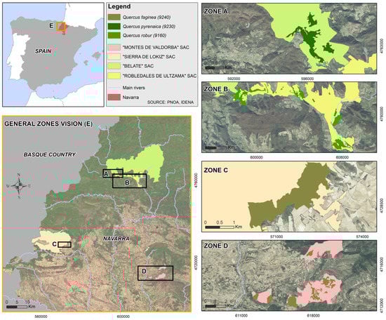
Figure 1.
Distribution of Zones A, B, C, and D in the Navarra region. The backdrop corresponds to a high spatial resolution orthophotography. Source: PNOA Spatial Data Infrastructure (SDI).
Zone A includes 135 ha of Galician-Portuguese forest dominated by Quercus robur (9160) and Quercus pyrenaica (9230). It is located within the SAC “Belate” (ES2200018), characterized by the uniqueness and diversity of habitats, flora, and fauna, which have been recognized through its protection in the Habitats Directive. According to the Digital Climatic Atlas of the Iberian Peninsula (DCAIP) [35], the average annual temperature in this area is 13 °C, and the annual precipitation ranges from 1000 to 1300 mm. Forests extend from the limits of Quinto Real to Usategieta in Leitza. Pyrenean oaks comprise relatively poor and open forests, with a distinctive acidophilic flora (Acer sp., Sorbus sp., Ilex aquifolium, Crataegus monogyna, i.e.,). Habitat Quercus pyrenaica (9230) is found on acidic substrates with elevations ranging between 400 and 1600 m above sea level (a.s.l.) and slopes ranging from 20% to more than 40% [36].
Zone B covers 314 ha of sub-Atlantic and Central European oak-hornbeam forests (Quercus robur habitat, 9160). The oak grove forests are managed by the Ultzama and Basaburua valley plans (ES2200043) and have been recognized through their protection as a Natura 2000 special area of conservation. Forests are characterized by deep and hydromorphic soils. Silty or clay-silty rocks dominate the lithology, whose limited extension prevents the existence of a specific fauna, such as Rana dalmatina or the middle-spotted woodpecker (Dendrocopos medius) [37], though the habitat serves as a refuge for other species, typical of deciduous forests or nearby habitats. The elevation ranges from 500 to 700 m a.s.l., and the slope steepness ranges from 2–3% to 0.4–0.5%. The lithology is mainly composed of washed brown earth acids [38].
In this area, the annual mean precipitation reaches approximately 1347 mm, and the average annual temperature is 13 °C. Forests are characterized by a smooth topography, with elevations below 400 m.
Zones C and D include 533 ha of Iberian oak forests of Quercus faginea and Q. canariensis. These zones are located within the “Montes de Valdorba” (ES2200322) and “Sierra de Lokiz” (ES2200022) SACs, which have a management plan for monitoring the conservation status of Quercus faginea habitat. Forests are dominated by Quercus faginea, which lives on neutral substrates between 500 and 1500 m a.s.l. In “Sierra de Lokiz”, the annual precipitation ranges from 800 to 1200 mm, and the average annual temperature varies from 10 °C to 12 °C [39]. However, in “Montes de Valdorba” the average annual temperature is 12.5 °C, and precipitation ranges from 600 to 900 mm.
3. Materials and Methods
A four-step methodology was conducted to classify and map the conservation status of oak grove habitats, Quercus robur, Quercus pyrenaica, and Quercus faginea (codes 9160, 9230, and 9240, respectively) (Figure 2). Initially, Sentinel-2 and LiDAR data were gathered and processed to develop radiometric indices and LiDAR metrics related to biodiversity. Furthermore, to cover the variability of the study sites, a representative random sample was created. In a third step, the Kruskal–Wallis and Dunn statistical tests were used to compare conservation status. Finally, the most suitable variables with an ecological significance were selected to classify and map the conservation status.
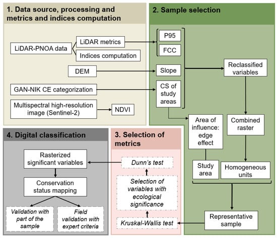
Figure 2.
Methodological scheme.
3.1. Conservation Status Reference Data
Navarra’s provincial community carried out its own habitat inventory (2004) of the areas included in the Natura 2000 Network. It was executed taking as a reference the enclosures of Crop and Exploitation Map (MCA) at a 1/25,000 scale. The data derived from the qualitative evaluation of conservation status carried out between 2004 and 2010 [36,40] were used for the analysis. The conservation status was classified into three categories: 1. unfavorable-bad (UB); 2. unfavorable-inappropriate (UI); and 3. favorable (F).
Habitats in the favorable status category are mature forests with a balanced distribution of tree ages and size classes. The forests may have open gaps due to the fall of old trees, favoring natural regeneration. The stands present little sign of human activity, raising their ecological value and microhabitat presence. There is also a high presence of dead wood on the ground or standing in various states of decomposition.
Unfavorable-inappropriate status integrates forests with a closed canopy, but older trees have not reached mature age yet. Dense regrowth of young trees in high competition for light could be found below the main canopy. The presence of standing dead wood of a small diameter is mainly due to young trees’ mortality.
The unfavorable-bad status category is characterized by a predominance of young trees originated from seed that form a forest in an initial state of succession, although stump or root sprouts are also frequent. Habitats resemble young forests, generally with lower canopy density and a lower amount of dead wood, generated by encroachment or large forest clearings.
3.2. ALS and Sentinel-2 Data Description
In this section, we describe the ALS and Sentinel-2 datasets used in this work. The ALS data were captured in 2017 by the Spanish National Plan for Aerial Orthophotography (PNOA) using a Single Photon LiDAR (SPL100). The SPL100 operates at a wavelength of 532 nm and collects up to 6 million points per second, with an average pulse repetition frequency of 60 KHz and a flying altitude between 3,500 and 6,000 m above the ground. Its maximum scanning angle is 25° and RMSE obtained in Z values was 6–10 cm. Point clouds, with a density of 14 points per m2, were provided in 1 × 1 km tiles in LAS format in European Terrestrial Reference System (ETRS) 1989 Universal Transverse Mercator (UTM) and orthometric heights [41]. A total of 80 LAS files, publicly available at the CNIG Download Centre and at the Spatial Data Infrastructure of Navarra (IDENA), were selected to cover the extension of the Zones A, B, C, and D.
The cloud-free image from the Sentinel-2A/B MSI sensor, of medium-high spatial resolution, and captured on 26th September 2019, was obtained from the European Space Agency’s (ESA) Sentinel Scientific Data Hub (https://scihub.copernicus.eu/) with a processing Level-2A that refers to the bottom of the atmosphere (BOA), being atmospherically and topographically corrected.
3.3. ALS Data Processing and Metrics Computation
The return heights of the point clouds were normalized using FUSION LDV 4.0 open-source software [42] by subtracting the elevation data from a digital elevation model (DEM) with 2 m grid resolution, provided by IDENA.
A complete set of statistical metrics, related to vertical and horizontal structure metrics commonly used within forestry, were generated using FUSION LDV 4.0 at a spatial resolution of 20 m, due to the regional scale of the analysis and to better match the spatial resolution of Sentinel-2 data. Following Domingo et al. [26], a threshold value of 0.2 m height was applied to remove understory and ground returns, considering also the RMSE in Z values of ALS-PNOA data. Metrics related to vegetation height include different intervals of return distribution percentiles (P01, P05, P10, P20, P30, P40, P50, P60, P70, P75, P80, P90, P95, and P99), the minimum, maximum, median, and mode of height distribution (Elev.min, Elev.max, Elev.mean, and Elev.mode), quadratic and cubic elevation (Elev. SQRT mean SQ, Elev. CUR mean CUBE), and several L moments (Elev. L1, Elev. L2, Elev. L3). L moments are canopy height metrics computed using linear functions of ordered data that suffer less from sample variability and are more robust to outliers in the data [30]. The computed metrics related to vegetation height variability correspond to skewness (Elev.skewness), kurtosis (Elev.kurtosis), coefficient of variation (Elev.CV), variance (Elev.variance), standard deviation (Elev. SD), and interquartile distance (Elev.IQ). Metrics related to canopy cover include the percentage of first or all returns above a threshold, the canopy relief ratio (CRR), the mean or the mode (e.g., % first ret. above 0.20), the percentage of all returns with a range of 0.5 m (e.g., % all ret. between 1 and 1.5 m), and the ratio of all returns with respect to the number of total returns (e.g., (all ret. above 0.20)/(total first ret.) by 100)).
Furthermore, the return proportion at every 0.5 m was computed as a measure of strata density. The strata metrics were used to subsequently compute two structural diversity indexes. The LHEI (LiDAR height evenness index), which is an adaptation of the Pielou’s index, and the LHDI (LiDAR height diversity index), which resembles the Shannon-Weiner diversity index. According to Listopad et al. [15], these structural diversity indices constitute valuable surrogates for structural and species biodiversity, allowing the development of ecosystem-specific parameters as quantifiable targets for ecosystem conservation. The two structural diversity indexes were computed by applying the formulas proposed by Listopad et al. [15] in R software (see Equations (1) and (2)).
where p is the proportion of returns every 0.5 m (h).
3.4. Sentinel-2 Data Processing and NDVI Derivation
The normalized differential vegetation index (NDVI) has been derived from Sentinel-2A images that have been atmospherically corrected (level 2A) using SNAP software (Sentinel toolboxes: https://step.esa.int/main/download/snap-download/). According to Equation (3), the red band related to chlorophyll absorption (Band 4) and the relatively high reflectance in the near infrared (NIR) (Band 8) of vegetation are used to calculate the NDVI.
3.5. Sample Selection
A sample of the data was selected in order to reduce computational effort, avoid overfitting the model, and have better control over the results. The variability of the forest was considered using a representative sample stratified using four variables: (1) canopy cover (using the FCC metric), (2) terrain slope, (3) canopy height (using the P95 metric), and (4) conservation status of the habitats, obtained through stratified random sampling [43].
Four classes have been established with respect to canopy cover (FCC), ranging from open or treeless spaces to high forest stand densities (see Table 1). Considering that there is no standard categorization for all habitats and that FCC varies according to local ecological characteristics within each biogeographic region [6], we defined four FCC ranges.

Table 1.
Ranges established for the variables FCC (%) and slope (%). Additionally, 9160 is Quercus robur habitat, 9230 is Quercus pyrenaica habitat, and 9240 is Quercus faginea habitat.
The slope of the terrain was obtained from the DEMs available in the spatial data infrastructure of Navarra (IDENA), used in the normalization of the point cloud. For this variable, three categories commonly used in its cartographic expression were established (see Table 1), differentiating between gentle, medium, and steep slopes.
P95 is related to a standard forest’s dominant height and, in turn, provides information about the age and condition of the stand. As can be seen in Table 2, P95 was categorized into four classes, referring to the age and condition of the forest stands in the three habitats to be analyzed. The P95 thresholds vary according to the habitat by considering the morphological characteristics of the forest stands.
Table 2.
Ranges established for the variable P95 (m). Additionally, 9160 is Quercus robur habitat, 9230 is Quercus pyrenaica habitat, and 9240 is Quercus faginea habitat.
The categorization created by GAN-NIK [36] in three classes in relation to the conservation status of the different habitats was used: from number 1 for the most poorly conserved habitats to number 3 for those in an optimal conservation status.
The mapping of the LiDAR-derived variables was generated from the LiDAR-PNOA data building raster layers with a 20-m resolution. All the variables were reclassified in a geographical information system (GIS), using ArcGIS software (https://www.esri.com/en-us/home), and overlapped to generate one layer. A total of 1000 random points in habitats Quercus robur (9160) and Quercus faginea (9240), and 450 in habitat Quercus pyrenaica (9230) were created, considering a minimum distance of 20 m between random points.
Finally, after the first statistical analysis, some of the sample points considered outliers, potentially linked to changes or data mismatches, were visited in the field in August 2020 in order to check the conservation status class assigned. A total of 150 points were distributed among the three sites that were visited. The agreement between the classification of the conservation status reference data and the field was approximately 50%. The misclassified points were reclassified for subsequent analyses.
3.6. Assessment of the Suitability of ALS Metrics for Conservation Status Discrimination
Preliminary analysis determined the absence of normality in the data. The transformation of the data to a logarithmic decimal scale was accomplished as a feasible alternative for normalizing the data. However, the Shapiro–Wilk test performed in an R environment revealed that a normal distribution was not reached (p-value < 0.05). Accordingly, the nonparametric Kruskal–Wallis test was computed in R [44,45] to select the LiDAR variables that were subsequently included in the classification process. The final selection of variables was created based on the presence of significant differences in the medians of the subgroups (p-value < 0.01) and their ecological significance, according to previous literature. Finally, the Dunn’s test of multiple comparisons was performed in R to pinpoint existing differences in each selected variable between the different categories of conservation.
3.7. Digital Classification of Conservation Status
The performance of two frequently used nonparametric machine-learning classification methods was tested to classify conservation status: SVM and RF. SVM was computed using radial (SVMr) and linear (SVMl) kernels. The SVM cost parameter was parametrized within an interval of 1–1000 and gamma within 0.01–1. The RF classifier was parametrized by applying between 1 and 3,000 trees to growth (ntrees) and between 1 and 3 metrics in each node (mtry), in accordance with Rodrigues et al. [46], and bias was corrected. The models were computed in an R environment using “e1071”, “randomForest” [47] and “caret” [48] for SVM and RF, respectively.
The classification was carried out using training and testing datasets based on a random sample of pixels (see the sample data section). Models were validated using the testing dataset, computed by applying a stratified random sampling of 30% to include the different conservation status. To increase robustness in the results, the validation was executed 100 times, and average performance values were computed [49]. In order to compare and, subsequently, determine the best classification model, the classification confusion matrices, user’s and producer’s accuracy, and overall accuracy were assessed [50]. The analysis of the results using LiDAR metrics on their own and in combination with the NDVI index was also performed.
4. Results
4.1. Suitability of the ALS Metrics for Conservation State Discrimination
Table 3 shows a selection of ALS metrics with the highest chi-square values after performing the nonparametric Kruskal–Wallis test. The FCC, LHEI, and LHDI biodiversity indices present the highest significant differences between conservation status in habitats Quercus robur (9160) and Quercus pyrenaica (9230). However, the total percentage of returns above mean (%RM), the height coefficient of variation (CV), 95th (P95), and 99th (P99) percentiles of height were significantly different between conservation status in habitats Quercus robur (9160) and Quercus faginea (9240), but not in habitat Quercus pyrenaica (9230). Furthermore, significant differences were observed in the elevation variance, the minimum, maximum and average elevation, and the mean absolute height deviation for all habitats.
Table 3.
Results of the Kruskal–Wallis test for habitats 9160, 9240, and 9230. *: p-value < 0.05; **: p-value < 0.01; ***: p-value < 0.001; NS: non-significant. Additionally, 9160 is Quercus robur habitat, 9230 is Quercus pyrenaica habitat, and 9240 is Quercus faginea habitat.
Concerning the ecological significance of all these variables, FCC is often used as a conservation status indicator of a forest habitat [36]. A value of 70% is considered a good, conserved forest; 40–70% means the conservation status is inadequate-unfavorable; and 20–40% is typical of a forest in a bad state of conservation. Following the criteria applied by GAN-NIK [36], below 20%, the formation cannot be considered a “forest”.
When age structure is applied to the dominant tree species and measured through parameters such as basal diameter, growth rings, or height, it provides information on diversity [51], the community structure, the population structure, and the successional status. To make an approximation of the structure and the age of the analyzed forest masses, P95 and the coefficient of variation of height were selected. With respect to the P95, it reflects the dominant height better than the average height, showing a 3-m error in past studies once validated in the field [52]. On the other hand, the coefficient of variation shows a dispersion degree in the elevation of the returns. This provides information about the variability of heights that exists in a determined patch, reflecting the variety of ages within the forest mass. It is possible that the old monospecific plantations provide similar values of average height to those of the well-preserved forests, although these plantations do not occur in this study.
LiDAR can approximate the quantification of old trees by estimating the percentage of early returns (or all returns) that are above the average height. In this study, the percentage was used instead of the total number of returns since several returns can correspond to the same tree and the density of points in the cloud is not homogeneous.
The kurtosis provides information about the community and the population structure, in addition to the successional state, and can be measured directly by LiDAR data.
After analyzing the ecological significance of all these variables, the following were selected for the subsequent classification process: 1) LHEI, LHDI, P95, FCC, CV, and percentage of returns above the mean (%RM) variables in habitats Quercus robur (9160) and Quercus faginea (9240); 2) LHEI, LHDI, and FCC variables in habitat 9230. Table 4 shows the results of Dunn’s test of multiple comparisons to pinpoint significant differences for each selected variable between conservation statuses.
Table 4.
Dunn’s test results for habitats 9160, 9240, and 9230. *: p-value < 0.05; **: p-value < 0.01; ***: p-value < 0.001; NS: non-significant. Additionally, 9160 is Quercus robur habitat, 9230 is Quercus pyrenaica habitat, and 9240 is Quercus faginea habitat.
In habitats Quercus robur (9160) and Quercus faginea (9240), the differences in the ecological variables were statistically significant in all conservation status classes with a confidence interval of 95%. However, Dunn’s test reflects the similarity of FCC data between the unfavorable-inappropriate and favorable categories (3–2) in habitat 9230, which determines no significant differences between these categories. On the other hand, in the case of the variables LHEI and LHDI, the differences between classes have a reliability above 95%. No significant changes were reported for the variables P95, CV, and %RM between the different categories in habitat 9230. The differences between conservation status classes for three significant variables have been represented graphically for each of the habitats using box plots (Figure 3 and Figure 4). These graphs show the distribution of the values of these variables within the three habitats for the different conservation status classes, while fluctuating points represent individual observations.
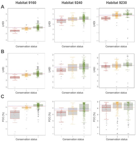
Figure 3.
Box plot diagrams of the significant variables (A) LHDI, (B) LHEI, and (C) FCC (%) between conservation status for habitats 9160, 9240, and 9230. The dashed blue line denotes the median, and the dotted red line is the average mean. 1: unfavorable-bad status (red); 2: unfavorable-inappropriate status (yellow); 3: favorable status (green). Additionally, 9160 is Quercus robur habitat, 9230 is Quercus pyrenaica habitat, and 9240 is Quercus faginea habitat.
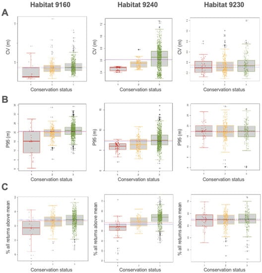
Figure 4.
Box plot diagrams of the variables (A) CV (m), (B) P95 (m), and (C) % of all returns above the mean between the different conservation statuses for habitats 9160, 9240, and 9230. The dashed blue line denotes the median, and the dotted red line is the average mean. 1: unfavorable-bad status (red); 2: unfavorable-inappropriate status (yellow); 3: favorable status (green). Additionally, 9160 is Quercus robur habitat, 9230 is Quercus pyrenaica habitat, and 9240 is Quercus faginea habitat.
4.2. Conservation Status Classification
Table 5 shows the comparison between classification methods, using the selected LiDAR metrics from the previous step. The models for habitat Quercus robur (9160) and Quercus faginea (9240) included seven ALS metrics: P95, CV, FCC, the percentage of all returns above mean, LHDI, and LHEI. The models for habitat 9230 included three ALS metrics: FCC, LHDI, and LHEI. The best classification method was RF, with an overall classification accuracy after validation of 83.01, 75.51, and 88.25 for habitats Quercus robur (9160), Quercus pyrenaica (9230), and Quercus faginea (9240), respectively (Table 5). The model was tuned with 500 trees and two metrics in each node. Lower accuracies were obtained with SVM with radial and linear kernels, which showed similar results between them, except for habitat 9230, where the radial kernel method obtained better results in comparison to the linear one. SVM was parametrized with a cost value of 100 and a gamma value of 0.15.
Table 5.
Comparison between classification methods using LiDAR metrics. The results refer to the overall accuracy of the three habitats. Additionally, 9160 is Quercus robur habitat, 9230 is Quercus pyrenaica habitat, and 9240 is Quercus faginea habitat.
Table 6 shows the comparison between classification methods using the selected LiDAR metrics and the NDVI from Sentinel-2. The results are similar, with almost unappreciable differences, being slightly better in habitat Quercus faginea (9230) and slightly worse in habitats Quercus robur (9160) and Quercus faginea (9240). The results denote that NDVI from Sentinel-2 does not have a high explanatory power for conservation status classification.
Table 6.
Comparison between classification methods using LiDAR and Sentinel metrics. The results refer to the overall accuracy of the three habitats. Additionally, 9160 is Quercus robur habitat, 9230 is Quercus pyrenaica habitat, and 9240 is Quercus faginea habitat.
According to the results shown in Table 7, Table 8 and Table 9, derived from the validation sample, the major confusion is observed between conservation status 2 and conservation status 3 for the habitats Quercus robur (9160) and Quercus pyrenaica (9230), while, for Quercus faginea (9240) habitat, higher confusion is found between conservation status 1 and conservation status 2.
Table 7.
Confusion matrix for the most accurate classification model using ALS data after validation for habitats 9160. Values are shown in %. CS stands for conservation status. Additionally, 9160 is Quercus robur habitat, 9230 is Quercus pyrenaica habitat, and 9240 is Quercus faginea habitat.
Table 8.
Confusion matrix for the most accurate classification model using ALS data after validation for habitats 9230. Values are shown in %. CS stands for conservation status. Additionally, 9160 is Quercus robur habitat, 9230 is Quercus pyrenaica habitat, and 9240 is Quercus faginea habitat.
Table 9.
Confusion matrix for the most accurate classification model using ALS data after validation for habitat 9240. Values are shown in %. CS stands for conservation status. Additionally, 9160 is Quercus robur habitat, 9230 is Quercus pyrenaica habitat, and 9240 is Quercus faginea habitat.
5. Discussion
Monitoring conservation status in special areas of conservation (SACs) is compulsory for all European member states, which was traditionally performed by using photo interpretation techniques and fieldwork. These practices present high economic and human costs, requiring the development of efficient alternatives on a larger spatial scale. The results reveal the suitability of single-photon LiDAR data for classifying conservation status in Quercus faginea (9240), Quercus pyrenaica (9230), and Quercus robur (9160) habitats under the Habitats Directive.
LHEI, LHDI, P95, FCC, CV, and percentage of returns above the mean (PRAM) were the most suitable LiDAR metrics to pinpoint the differences between conservation statuses in Quercus robur (9160) and Quercus faginea (9240) habitats. Though LHEI, LHDI, and FCC LiDAR metrics were the most relevant in the Quercus pyrenaica 9230 habitat, these results are in accordance with Zlinszky et al. [24], who determined that the selected variables depend on the habitat type. The selected variables provide direct or indirect information on FCC, age, presence of old trees, diversity, structural complexity, and strata development. This seems to indicate that LiDAR metrics and structural diversity indices provide suitable information about conservation status and ecological characteristics [15]. Our results are in accordance with Gelabert et al. [12], who concluded that structural diversity indexes, such as LHDI and canopy height variability metrics, were suitable for depicting structural differences in Mediterranean Pinus halepensis forests affected by fires occurring on different dates. On the contrary, unlike the good results obtained by Valbuena et al. [27] in the use of the L-moments to quantify the complexity of the canopy and classify the structure of the boreal forest according to its ecological function, in our case, no significant differences were found with respect to the conservation status estimation.
The classification results show the feasibility of single-photon LiDAR to discriminate conservation status in oak grove forests with an accuracy after validation of 83.01%, 75.51%, and 88.25% for Quercus robur (9160), Quercus pyrenaica (9230), and Quercus faginea (9240) habitats, respectively. Our model results have comparable accuracies to previous studies that classified the conservation status in grasslands [53,54], steppes [24], or heatlands [55] using LiDAR or hyperspectral data or their combinations, which range roughly from 70% to 89%. Though this comparison should be interpreted with caution as the habitat type was different, the lower penetrability of the SPL data appears to be complemented by the high density of points in the data source. The use of LiDAR data was in accordance with Simonson et al. [25], who showed the applicability of three-dimensional data sources to predict conservation status indicators in Quercus suber habitats in Portugal. A potential handicap of our approach could have been the discrepancy in dates between the ALS data (2017) and the conservation status categorization (2004–2010). However, the conservation status does not vary rapidly over time, and there was good agreement in classification status in the plots visited in the field in 2020, which potentially were affected by structural changes, supporting the usefulness of the selected approach and associated accuracies for conservation status classification. The best classification method for all the habitats, independent of the sample size and the number of variables included in the classification, was RF, in agreement with Marcinkowska-Ochtyra et al. [54]. Furthermore, our results also suggest that radial kernels work better than linear kernels in the SVM classifier, agreeing with Domingo et al. [26] and Gelabert et al. [12].
Concerning the combination of passive and active sensors, several authors have successfully integrated hyperspectral and LiDAR for grassland habitat mapping. Furthermore, multispectral and LiDAR data have also been combined for forest structural variable characterization. For example, Alonso-Benito et al. [56] reported an improvement of 10% in the overall accuracy of fuel type mapping when combining World View-2 and LiDAR data, and Mutlu et al. [57] pointed out an improvement of 14% when combining QuickBird and LiDAR data. However, our results showed that the inclusion of the NDVI index from a Sentinel-2A image did not significantly improve the classification accuracy, in accordance with Domingo et al. [26], who concluded that ALS-derived metrics have more importance in fuel model classification than multispectral Sentinel-2 data, which added a minor improvement in fuel type classification accuracy.
Future research should focus on testing the performance of further structural diversity indices, such as rumple, which were successfully used to characterize structural complexity [58] and generate parsimonious models in fuel type mapping [26]. In addition, further analysis should consider other habitat types, including grasslands and shrublands, to better provide regional-scale approaches for conservation status monitoring.
6. Conclusions
The three-dimensional structure of natural habitats is essential for monitoring the conservation status of the Natura 2000 Network. The results of the present research verify the usefulness of single-photon LiDAR together with machine learning algorithms to classify three conservation status categories in oak grove habitats. Five LiDAR-derived metrics (LHEI, LHDI, P95, FCC, CV, and PRAM) were the most suitable variables for pinpointing the differences between conservation status, while Sentinel-2-derived NDVI did not significantly improve model accuracy. The RF method produced the most accurate classifications of conservation status, with values after validation of 83.01%, 75.51%, and 88.25% for Quercus robur (9160), Quercus pyrenaica (9230), and Quercus faginea (9240) habitats, respectively. The characterization of conservation status as an essential biodiversity variable at a regional scale is paramount for continuous protected area monitoring, constituting a relevant input to define sustainable conservation actions by forest managers.
Author Contributions
Conceptualization, A.G.-G., M.T.L. and D.D.; methodology, M.T.L. and D.D.; validation, A.G.-G., M.T.L. and D.D.; formal analysis, A.G.-G., M.T.L. and D.D.; writing—original draft preparation, A.G.-G., M.T.L. and D.D.; writing—review and editing, A.G.-G., M.T.L. and D.D. All authors have read and agreed to the published version of the manuscript.
Funding
This research did not receive any specific grant from funding agencies in the public, commercial, or not-for-profit sectors.
Data Availability Statement
The data that support the findings of this study are openly available in Mendeley data at http://doi.org/10.17632/gpy8kydxx7.1, reference Lamelas, Maria Teresa; Domingo, Darío; García-Galar, Aitor (2021), “LiDAR metrics and Sentinel-2 derived NDVI for Conservation Status Mapping”, Mendeley Data, V1.
Acknowledgments
The author acknowledges the support through the Postdoc Margarita Salas grant funded by the European Union-Next GenerationEU to Dario Domingo (MS-240621).
Conflicts of Interest
The authors declare no conflict of interest.
References
- Pressey, R.L.; Cabeza, M.; Watts, M.E.; Cowling, R.M.; Wilson, K.A. Conservation Planning in a Changing World. Trends Ecol. Evol. 2007, 22, 583–592. [Google Scholar] [CrossRef] [PubMed]
- Margules, C.R.; Pressey, R.L. Systematic Conservation Planning. Nature 2000, 405, 243–253. [Google Scholar] [CrossRef] [PubMed]
- Maiorano, L.; Falcucci, A.; Garton, E.O.; Boitani, L. Contribution of the Natura 2000 Network to Biodiversity Conservation in Italy. Conserv. Biol. 2007, 21, 1433–1444. [Google Scholar] [CrossRef]
- European Commission. Interpretation Manual of European Union Habitats; European Commission: Brussels, Belgium, 2013. [Google Scholar]
- Vanden Borre, J.; Paelinckx, D.; Mücher, C.A.; Kooistra, L.; Haest, B.; De Blust, G.; Schmidt, A.M. Integrating Remote Sensing in Natura 2000 Habitat Monitoring: Prospects on the Way Forward. J. Nat. Conserv. 2011, 19, 116–125. [Google Scholar] [CrossRef]
- Garcia, S.; Alvarez, J.; Pozo, I. Selection of Natura 2000 Sites Using Systematic Conservation Planning. In A Methodological Proposal for Turkey; EuropeAid/134319/IH/SER/TR; Hulla & Co. Human Dynamics: Vienna, Austria, 2018. [Google Scholar]
- Pettorelli, N.; Wegmann, M.; Skidmore, A.; Mücher, S.; Dawson, T.P.; Fernandez, M.; Lucas, R.; Schaepman, M.E.; Wang, T.; O’Connor, B.; et al. Framing the Concept of Satellite Remote Sensing Essential Biodiversity Variables: Challenges and Future Directions. Remote Sens. Ecol. Conserv. 2016, 2, 122–131. [Google Scholar] [CrossRef]
- Zlinszky, A.; Deák, B.; Kania, A.; Schroiff, A.; Pfeifer, N. Biodiversity Mapping via NATURA 2000 Conservation Status and EBV Assessment Using Airborne Laser Scanning in Alkali Grasslands. Int. Arch. Photogramm. Remote Sens. Spat. Inf. Sci. 2016, 41, 1293–1299. [Google Scholar] [CrossRef]
- Kimmins, J.P. Biodiversity and Its Relationship to Ecosystem Health and Integrity. For. Chron. 1997, 73, 229–232. [Google Scholar] [CrossRef]
- McElhinny, C.; Gibbons, P.; Brack, C.; Bauhus, J. Forest and Woodland Stand Structural Complexity: Its Definition and Measurement. For. Ecol. Manag. 2005, 218, 1–24. [Google Scholar] [CrossRef]
- Smith, G.F.; Gittings, T.; Wilson, M.; French, L.; Oxbrough, A.; O’Donoghue, S.; O’Halloran, J.; Kelly, D.L.; Mitchell, F.J.G.; Kelly, T.; et al. Identifying Practical Indicators of Biodiversity for Stand-Level Management of Plantation Forests. Biodivers. Conserv. 2008, 17, 991–1015. [Google Scholar] [CrossRef]
- Gelabert, P.J.; Montealegre, A.L.; Lamelas, M.T.; Domingo, D. Forest Structural Diversity Characterization in Mediterranean Landscapes Affected by Fires Using Airborne Laser Scanning Data. GISci. Remote Sens. 2020, 57, 497–509. [Google Scholar] [CrossRef]
- Zimble, D.A.; Evans, D.L.; Carlson, G.C.; Parker, R.C.; Grado, S.C.; Gerard, P.D. Characterizing Vertical Forest Structure Using Small-Footprint Airborne LiDAR. Remote Sens. Environ. 2003, 87, 171–182. [Google Scholar] [CrossRef]
- Brokaw, N.V.L.; Lent, R.A. Vertical Structure. In Maintaining Biodiversity in Forest Ecosystems; Cambridge University Press: Cambridge, UK.
- Listopad, C.M.C.S.; Masters, R.E.; Drake, J.; Weishampel, J.; Branquinho, C. Structural Diversity Indices Based on Airborne LiDAR as Ecological Indicators for Managing Highly Dynamic Landscapes. Ecol. Indic. 2015, 57, 268–279. [Google Scholar] [CrossRef]
- Hyde, P.; Dubayah, R.; Walker, W.; Blair, J.B.; Hofton, M.; Hunsaker, C. Mapping Forest Structure for Wildlife Habitat Analysis Using Multi-Sensor (LiDAR, SAR/InSAR, ETM+, Quickbird) Synergy. Remote Sens. Environ. 2006, 102, 63–73. [Google Scholar] [CrossRef]
- Hill, R.A.; Hinsley, S.A. Airborne Lidar for Woodland Habitat Quality Monitoring: Exploring the Significance of Lidar Data Characteristics When Modelling Organism-Habitat Relationships. Remote Sens. 2015, 7, 3446–3466. [Google Scholar] [CrossRef]
- Goetz, S.; Steinberg, D.; Dubayah, R.; Blair, B. Laser Remote Sensing of Canopy Habitat Heterogeneity as a Predictor of Bird Species Richness in an Eastern Temperate Forest, USA. Remote Sens. Environ. 2007, 108, 254–263. [Google Scholar] [CrossRef]
- Clawges, R.; Vierling, K.; Vierling, L.; Rowell, E. The Use of Airborne Lidar to Assess Avian Species Diversity, Density, and Occurrence in a Pine/Aspen Forest. Remote Sens. Environ. 2008, 112, 2064–2073. [Google Scholar] [CrossRef]
- Bergen, K.M.; Goetz, S.J.; Dubayah, R.O.; Henebry, G.M.; Hunsaker, C.T.; Imhoff, M.L.; Nelson, R.F.; Parker, G.G.; Radeloff, V.C. Remote Sensing of Vegetation 3-D Structure for Biodiversity and Habitat: Review and Implications for Lidar and Radar Spaceborne Missions. J. Geophys. Res. Biogeosci. 2009, 114. [Google Scholar] [CrossRef]
- Nelson, R.; Keller, C.; Ratnaswamy, M. Locating and Estimating the Extent of Delmarva Fox Squirrel Habitat Using an Airborne LiDAR Profiler. Remote Sens. Environ. 2005, 96, 292–301. [Google Scholar] [CrossRef]
- Johnston, A.N.; Moskal, L.M. High-Resolution Habitat Modeling with Airborne LiDAR for Red Tree Voles. J. Wildl. Manag. 2017, 81, 58–72. [Google Scholar] [CrossRef]
- Guo, X.; Coops, N.C.; Tompalski, P.; Nielsen, S.E.; Bater, C.W.; John Stadt, J. Regional Mapping of Vegetation Structure for Biodiversity Monitoring Using Airborne Lidar Data. Ecol. Inform. 2017, 38, 50–61. [Google Scholar] [CrossRef]
- Zlinszky, A.; Deák, B.; Kania, A.; Schroiff, A.; Pfeifer, N. Mapping Natura 2000 Habitat Conservation Status in a Pannonic Salt Steppe with Airborne Laser Scanning. Remote Sens. 2015, 7, 2991–3019. [Google Scholar] [CrossRef]
- Simonson, W.D.; Allen, H.D.; Coomes, D.A. Remotely Sensed Indicators of Forest Conservation Status: Case Study from a Natura 2000 Site in Southern Portugal. Ecol. Indic. 2013, 24, 636–647. [Google Scholar] [CrossRef]
- Domingo, D.; de la Riva, J.; Lamelas, M.T.; García-Martín, A.; Ibarra, P.; Echeverría, M.; Hoffrén, R. Fuel Type Classification Using Airborne Laser Scanning and Sentinel 2 Data in Mediterranean Forest Affected by Wildfires. Remote Sens. 2020, 12, 3660. [Google Scholar] [CrossRef]
- Valbuena, R.; Maltamo, M.; Mehtätalo, L.; Packalen, P. Key Structural Features of Boreal Forests May Be Detected Directly Using L-Moments from Airborne Lidar Data. Remote Sens. Environ. 2017, 194, 437–446. [Google Scholar] [CrossRef]
- Ackers, S.H.; Davis, R.J.; Olsen, K.A.; Dugger, K.M. The Evolution of Mapping Habitat for Northern Spotted Owls (Strix Occidentalis Caurina): A Comparison of Photo-Interpreted, Landsat-Based, and Lidar-Based Habitat Maps. Remote Sens. Environ. 2015, 156, 361–373. [Google Scholar] [CrossRef]
- North, M.P.; Kane, J.T.; Kane, V.R.; Asner, G.P.; Berigan, W.; Churchill, D.J.; Conway, S.; Gutiérrez, R.J.; Jeronimo, S.; Keane, J.; et al. Cover of Tall Trees Best Predicts California Spotted Owl Habitat. For. Ecol. Manag. 2017, 405, 166–178. [Google Scholar] [CrossRef]
- Hosking, J.R.M. L-Moments: Analysis and Estimation of Distributions Using Linear Combinations of Order Statistics. J. R. Stat. Soc. Ser. B 1990, 52, 105–124. [Google Scholar] [CrossRef]
- Adnan, S.; Maltamo, M.; Coomes, D.A.; García-Abril, A.; Malhi, Y.; Manzanera, J.A.; Butt, N.; Morecroft, M.; Valbuena, R. A Simple Approach to Forest Structure Classification Using Airborne Laser Scanning That Can Be Adopted across Bioregions. For. Ecol. Manag. 2019, 433, 111–121. [Google Scholar] [CrossRef]
- Shannon, C.; Weaver, W. The Mathematical Theory of Communications; University of Illinois Press: Urbana, IL, USA, 1949. [Google Scholar]
- Moreno, C. M&T—Manuales y Tesis SEAMétodos Para Medir La Biodiversidad; Sociedad Entomológica Aragones: Aragones, Spain, 2001; Volume 1, ISBN -8492249528. [Google Scholar]
- Lorda López, M.; Peralta de Andrés, J.; Berastegi, A.; Gómez, D. Síntesis de La Flora Vascular de Navarra. In Proceedings of the Actes del IX Col•loqui Internacional de Botànica Pirenaico-cantàbrica a Ordino, Ordino, Andorra, 7–9 July 2011; Volume 281, pp. 258–281. [Google Scholar]
- Ninyerola, M.; Pons, X.; Roure, J.M. Atlas Climático Digital de La Península Ibérica: Metodología y Aplicaciones En Bioclimatología y Geobotánica; Universitat Autònoma de Barcelona, Departament de Biologia Animal, Biologia Vegetal i Ecologia (Unitat de Botánica): Barcelona, Spain, 2005. [Google Scholar]
- GAN-NIK—Gestión ambiental Viveros y Repoblaciones de Navarra, S.A. Bases Técnicas Para El Plan de Gestión de La Zona Especial de Conservación (ZEC) (Belate, ES2200018); GAN-NIK—Gestión ambiental Viveros y Repoblaciones de Navarra, S.A.: Navarra, Spain, 2014. [Google Scholar]
- Bartolomé, C.; Álvarez Jiménez, J.; Vaquero, J.; Costa, M.; Casermeiro, M.A.; Giraldo, J.; Zamora, J.T. Los Tipos de Hábitat de Interés Comunitario de España. Guía Básica; Ministerio de Medio Ambiente, Dirección General para la Biodiversidad: Madrid, Spain, 2005. [Google Scholar]
- GAN-NIK—Gestión ambiental Viveros y Repoblaciones de Navarra, S.A. Bases Técnicas Para El Plan de Gestión Del Lugar de Importancia Comunitaria: Robledales de Ultzama y Basaburua (ES2200043): Descripción y Análisis Ecológico; GAN-NIK—Gestión ambiental Viveros y Repoblaciones de Navarra, S.A.: Navarra, Spain, 2006. [Google Scholar]
- GAN-NIK—Gestión ambiental Viveros y Repoblaciones de Navarra, S.A. Bases Técnicas Para El Plan de Gestión de La Zona Especial de Conservación (ZEC): Sierra de Lokiz (ES2200022); GAN-NIK—Gestión ambiental Viveros y Repoblaciones de Navarra, S.A.: Navarra, Spain, 2017. [Google Scholar]
- Olano, J.M.; Ferrer, V.; Peralta, J.; Remon, J.L.; Berastegi, A.; García, S. Cartografía de Hábitats En Los Lugares de Importancia Comunitaria (LICs) de Navarra (Red Natura 2000); Gestión del Patrimonio Natural: Navarra, Spain, 2003. [Google Scholar]
- Huarte Sanz, A. Clasificación de La Cobertura LiDAR 2017 de Navarra Con Inteligencia Artificial y Herramientas Open-Source. XIII Jornadas SIG Libre, SIGTE. Servei d’Informació Geogràfica i Teledetecció. Available online: https://dugi-doc.udg.edu/handle/10256/17286 (accessed on 29 May 2019).
- McGaughey, R.J. FUSION/LDV: Software for LIDAR Data Analysis and Visualization; Service, U.F., Ed.; Pacific Northwest Research Station: Seattle, WA, USA, 2018. [Google Scholar]
- Næsset, E.; Økland, T. Estimating Tree Height and Tree Crown Properties Using Airborne Scanning Laser in a Boreal Nature Reserve. Remote Sens. Environ. 2002, 79, 105–115. [Google Scholar] [CrossRef]
- Healy, M.J. Statistics from the inside. 12. Non-Normal Data. Arch. Dis. Child 1994, 70, 158. [Google Scholar] [CrossRef]
- Sainani, K.L. Dealing With Non-Normal Data. PMR 2012, 4, 1001–1005. [Google Scholar] [CrossRef]
- Rodrigues, M.; de la Riva, J. An Insight into Machine-Learning Algorithms to Model Human-Caused Wildfire Occurrence. Environ. Model. Softw. 2014, 57, 192–201. [Google Scholar] [CrossRef]
- Liaw, A.; Wiener, M. Classification and regression by randomForest. R News 2002, 2/3, 18–22. [Google Scholar]
- Van Essen, D.C.; Drury, H.A.; Dickson, J.; Harwell, J.; Hanlon, D.; Anderson, C.H. An Integrated Software Suite for Surface-Based Analyses of Cerebral Cortex. J. Am. Med. Inform. Assoc. 2001, 8, 443–459. [Google Scholar] [CrossRef] [PubMed]
- García-Gutiérrez, J.; Martínez-Álvarez, F.; Troncoso, A.; Riquelme, J.C. A Comparison of Machine Learning Regression Techniques for LiDAR-Derived Estimation of Forest Variables. Neurocomputing 2015, 167, 24–31. [Google Scholar] [CrossRef]
- Foody, G.M. Explaining the Unsuitability of the Kappa Coefficient in the Assessment and Comparison of the Accuracy of Thematic Maps Obtained by Image Classification. Remote Sens. Environ. 2020, 239, 111630. [Google Scholar] [CrossRef]
- Lähde, E.; Laiho, O.; Norokorpi, Y.; Saksa, T. Stand Structure as the Basis of Diversity Index. For. Ecol. Manag. 1999, 115, 213–220. [Google Scholar] [CrossRef]
- Magnussen, S.; Boudewyn, P. Derivations of Stand Heights from Airborne Laser Scanner Data with Canopy-Based Quantile Estimators. Can. J. For. Res. 1998, 28, 1016–1031. [Google Scholar] [CrossRef]
- Demarchi, L.; Kania, A.; Ciężkowski, W.; Piórkowski, H.; Oświecimska-Piasko, Z.; Chormański, J. Recursive Feature Elimination and Random Forest Classification of Natura 2000 Grasslands in Lowland River Valleys of Poland Based on Airborne Hyperspectral and LiDAR Data Fusion. Remote Sens. 2020, 12, 1842. [Google Scholar] [CrossRef]
- Marcinkowska-Ochtyra, A.; Gryguc, K.; Ochtyra, A.; Kopeć, D.; Jarocińska, A.; Sławik, Ł. Multitemporal Hyperspectral Data Fusion with Topographic Indices—Improving Classification of Natura 2000 Grassland Habitats. Remote Sens. 2019, 11, 2264. [Google Scholar] [CrossRef]
- Haest, B.; Vanden Borre, J.; Spanhove, T.; Thoonen, G.; Delalieux, S.; Kooistra, L.; Mücher, C.; Paelinckx, D.; Scheunders, P.; Kempeneers, P. Habitat Mapping and Quality Assessment of NATURA 2000 Heathland Using Airborne Imaging Spectroscopy. Remote Sens. 2017, 9, 266. [Google Scholar] [CrossRef]
- Alonso-Benito, A.; Arroyo, L.A.; Arbelo, M.; Hernández-Leal, P. Fusion of WorldView-2 and LiDAR Data to Map Fuel Types in the Canary Islands. Remote Sens. 2016, 8, 669. [Google Scholar] [CrossRef]
- Mutlu, M.; Popescu, S.; Stripling, C.; Spencer, T. Mapping Surface Fuel Models Using Lidar and Multispectral Data Fusion for Fire Behavior. Remote Sens. Environ. 2008, 112, 274–285. [Google Scholar] [CrossRef]
- Kane, V.R.; Bakker, J.D.; McGaughey, R.J.; Lutz, J.A.; Gersonde, R.F.; Franklin, J.F. Examining Conifer Canopy Structural Complexity across Forest Ages and Elevations with LiDAR Data. Can. J. For. Res. 2010, 40, 774–787. [Google Scholar] [CrossRef]
Disclaimer/Publisher’s Note: The statements, opinions and data contained in all publications are solely those of the individual author(s) and contributor(s) and not of MDPI and/or the editor(s). MDPI and/or the editor(s) disclaim responsibility for any injury to people or property resulting from any ideas, methods, instructions or products referred to in the content. |
© 2023 by the authors. Licensee MDPI, Basel, Switzerland. This article is an open access article distributed under the terms and conditions of the Creative Commons Attribution (CC BY) license (https://creativecommons.org/licenses/by/4.0/).