Multiple Sea Ice Type Retrieval Using the HaiYang-2B Scatterometer in the Arctic

Abstract

Sea ice type classification is of great significance for the exploration of waterways, fisheries, and offshore operations in the Arctic. However, to date, there is no multiple remote sensing method to detect sea ice type in the Arctic. This study develops a multiple sea ice type algorithm using the HaiYang-2B Scatterometer (HY-2B SCA). First, the parameters most applicable to classify sea ice type are selected through feature extraction, and a stacking model is established for the first time, which integrates decision tree and image segmentation algorithms. Finally, multiple sea ice types are classified in the Arctic, comprising Nilas, Young Ice, First Year Ice, Old Ice, and Fast Ice. Comparing the results with the Ocean and Sea Ice Satellite Application Facility (OSI-SAF) Sea Ice Type dataset (SIT) indicates that the sea ice type classified by HY-2B SCA (Stacking-HY2B) is similar to OSI-SAF SIT with regard to the changing trends in extent of sea ice. We use the Copernicus Marine Environment Monitoring Service (CMEMS) high-resolution sea ice type data and EM-Bird ice thickness data to validate the result, and accuracies of 87% and 88% are obtained, respectively. This indicates that the algorithm in this work is comparable with the performance of OSI-SAF dataset, while providing information of multiple sea ice types.

1. Introduction

Sea ice is among the most important climatic factors in the Arctic. It plays an important role in climate change and further affects the global climate state. Sea ice also regulates atmospheric and oceanic circulation by affecting ocean surface radiation, temperature, energy balance, and salt current circulation [1]. According to the classification standard of the World Meteorological Organization, sea ice can be categorized into Nilas, New Ice (NI), Young Ice (YI), First Year Ice (FYI), and multi-year ice (MYI) in the Arctic. [2]. Ice types have an important impact on assessing the total amount of sea ice. At present, most sea ice classifications sort sea ice into newly formed ice after summer (FYI) and ice that has survived at least one summer (MYI), while the relevant research on further ice type subdivision is very limited. However, along with the growing research on polar climate change, the demand for sea ice classification in the Arctic is growing, as it is of great significance in exploring Arctic waterways, fisheries, and offshore operations.

Initially, observing sea ice in polar regions was mostly based on aerial surveys and coastal observations, which were costly, time-sensitive, and had low observational space coverage. Boasting wide spatial coverage, high temporal resolution, and continuous observation capability, satellite observations are an important method for polar sea ice observation. Remote sensing of sea ice classification can be divided into two categories, namely microwave-based and optical-based remote sensing. Microwave scatterometer observations are one of the most important methods for sea ice classification. This is due to a lower density and more air bubbles in MYI, which leads to a backscatter coefficient (σ⁰) of MYI with strong volumetric scattering that is larger than that of FYI [3,4]. Therefore, sea ice can be distinguished based on the difference in σ⁰.

Numerous researchers have conducted studies on scatterometer sea ice classification. For Ku band scatterometers, Remund and Long [5] used QuikSCAT and Seawinds and proposed a method for ice and water detection, mainly based on the maximum likelihood estimation using the difference in polarization properties of sea ice and seawater. Kwok [6] used QuikSCAT data to develop an empirical algorithm for MYI quantile detection, employing a fixed threshold method to successfully distinguish between FYI and MYI and to calculate the proportion of image elements for MYI. Nghiem et al. [7] have developed a sea ice classification algorithm based on statistical analysis, showing two separate distinctive peaks in backscatter data for seasonal and perennial sea ice in freezing seasons. They used QuikSCAT data to classify Arctic sea ice into FYI, MYI, and mixed ice. Swan and Long [8] generated an Arctic sea ice classification dataset for 2002–2009 for different seasonal Arctic σ⁰ transformations using dynamic thresholds of seasonal transformations, also based on QuikSCAT data. Lindell and Long [9] derived and cross-referenced MYI quantile data from QuikSCAT and OSCAT-2. Li et al. [10] used Fisher’s linear discriminant method to distinguish sea ice from seawater in HY-2A scatterometer data. In the case of C-band scatterometers, in 1997, Early and Long [11] attempted to classify sea ice in the Southern Ocean based on the wide amplitude and wide incidence angle characteristics of an active microwave instrument (AMI) on board the ERS-1 satellite. Ezraty and Cavani [12] compared a microwave scatterometer, NSCAT, operating in the Ku band with a microwave scatterometer, AMI, operating in the C band, and showed that the difference in σ⁰ between FYI and MYI is larger in the Ku band than that in the C band in the Arctic. Lindell and Long [13] found that the difference in MYI and FYI σ⁰ was not obvious, which made it difficult to classify sea ice using only a C band scatterometer. Then, they combined ASCAT and SSMIS data by using Bayesian classifiers to achieve Arctic sea ice classification. Further passive microwave data have been introduced into some studies of sea ice classification based on C band and Ku band scatterometer data. Zhang et al. [14] used the backscatter coefficients and brightness temperatures from QuikSCAT/AMSR-E and ASCAT/AMSR-2 to classify sea ice using the K-means clustering algorithm to distinguish sea ice into MYI and 1-year-old ice; the classifications were consistent with results of visual interpretation from synthetic aperture radar images in the Canadian Arctic Archipelago with an overall classification accuracy of over 93%. In 2021, Zhang et al. [15] evaluated the relationship between the σ⁰ and the incident angle by comparing the trend in the σ⁰ of QSCAT, ASCAT, and RFSCAT with the same incident angle, and studied the classification results of these three scatterometers by using the adaptive sea ice classification algorithm based on K-means clustering algorithm; the overall accuracy was around 77% and 80% for the RFSCAT and ASCAT results, respectively.

In recent years, with the extensive application of deep learning in satellite remote sensing [16], some deep learning methods have been used for sea ice detection and classification based on scatterometers in polar regions. Ren et al. [17] employed the U-Net network for sea ice and open water classification using SAR images and integrated a double attention mechanism on the original U-Net network to improve the feature extraction performance. Han et al. [18] proposed a feature level fusion of heterogeneous data from SAR and optical images and proposed a feature extraction-based sea ice image classification method. Andersson et al. [19] designed the ICE-Net network structure by inputting CMIP6 simulated data and remote sensing observation data for Arctic sea ice prediction. The deep learning method for sea ice retrieval effectively identifies different features among different ice types and fully benefits from the advantages of a large amount of remote sensing data, a wide observation range, and a long time period. However, it has the disadvantage that it is easily affected by the selected training sample features, leading to overfitting. All the above algorithms commonly use the threshold method or classifier for the initial training of the classifier and then correct the results by image-level processing [20] to improve the model classification performance.

Considering the importance of the information for multiple sea ice type classification in the Arctic, and the fact that there is currently no satellite product of it, this study is dedicated to the algorithm development for multiple sea ice types in the Arctic using a HaiYang-2B Scatterometer (HY-2B SCA). First, we train the decision tree model and image segmentation model separately, then use the stacking algorithm to fuse these two models at the algorithm level, instead of using image-level correction, as most algorithms do. This is not an operational algorithm due to the use of dynamic threshold segmentation. There are many melt ponds above sea ice in the summer in the Arctic, which prevent the microwave signal from penetrating the ice; therefore, this research uses data from October 2019 to April 2020 and October 2020 to April 2021 as training datasets and October 2021 to April 2022 as the validation dataset.

2. Data and Methods

A variety of data and algorithms were employed in this study. The HY-2B SCA σ⁰ data were used for sea ice type retrieval [21]; Arctic and Antarctic Research Institute (AARI) ice map data [22] were used as reference data; OSI-SAF ice type data [23] and Ease-Grid Sea Ice Age data from the National Snow and Ice Data Center (NSIDC) [24] were selected as comparative data; and CMEMS data [25] and the EM-Bird ice thickness dataset [26] were used to validate the results.

2.1. Data

2.1.1. HY-2B Scatterometer Data

The HY-2B satellite is the first operational satellite in the marine dynamic environment satellite series from China. The satellite has a repetition period of 14 days with a sun-synchronous orbit spacing of 207.64 km, a sub-satellite point drift of ±1 km, an orbital inclination of 99.34015°, and a local time of 6:00 AM at the descending node. The HY-2B satellite carries a Ku band microwave scatterometer (HY-2B SCA), which is a rotating pencil beam scatterometer. The HY-2B SCA’s swath widths are 1350 KM and 1700 KM under H-polarization and V-polarization, respectively. The incidence angles of the HY-2B SCA are 41° under H-polarization and 48° under V-polarization. Additionally, the pole hole is at 88°N in the arctic [21].

The HY-2B SCA L2A σ⁰ dataset was provided by the National Satellite Ocean Application Service (NSOAS), with a resolution of 25 km. The observation accuracy of σ⁰ is 0.5 dB. The HY2B SCA σ⁰ data were projected into a 25 KM × 25 KM grid in a polar-beam projection on a daily basis, averaging daily images from 16–17 L2A data files. Data download to https://osdds.nsoas.org.cn/ (accessed on 19 April 2022). In this study, observed values of σ⁰ under VV polarization (${\mathsf{\sigma }}_{\mathrm{VV}}^0$) and HH polarization (${\mathsf{\sigma }}_{\mathrm{HH}}^0$) were used for Arctic sea ice classification. Figure 1 shows images of σ⁰ under two polarization modes.

2.1.2. AARI ICE Chart Products

The Arctic and Antarctic Research Institute (AARI) in St. Petersburg, Russia, produces weekly AARI ice maps in the polar regions [22], which are obtained from satellite data (visible, infrared, and radar) and data reported from coastal stations and ships. Since the 21st century, the main data source for the AARI has been satellite data. Since 2013, the satellite receiving site in Barentsburg (Spitzbergen) has carried out permanent reception and automatic processing of visual and IR data from NOAA, MetOp, Terra, Aqua, Suomi NPP, and Fengyun satellites; processed images are distributed to ice experts for further analysis [27]. It classifies five ice types: Nilas, YI, FYI, Old Ice, and Fast Ice. To store and export data, AWS “Ice expert” includes special tools to standardize vector charts according to WMO SIGRID-3 nomenclature [28]. The AARI dataset provides sea ice classification polygon data, whose coordinates were extracted and projected to a 25 KM grid in this study.

2.1.3. OSI-SAF SEA ICE TYPE Dataset

The OSI-SAF sea ice type product (Global Sea Ice Type, OSI-403-c) is provided by the European Organization for the Exploitation of Meteorological Satellites (EUMETSAT) [25], and its accuracy has been scientifically validated. The performance of the OSI-403-c product in the Northern Hemisphere is within the target accuracy requirements, which is 100,000 km² monthly STD of the daily differences from a running mean for all months, except in October 2019 [29]. It is based on a combination of passive and active microwave remote sensing data, calculated by a Bayesian algorithm, and provides sea ice type maps with a spatial resolution of 10 km in both hemispheres. The OSI-SAF provides two classifications, FYI and MYI, which correspond to areas with more than 30% sea ice concentration, while open water corresponds to areas with less than 30% sea ice concentration. The OSI SAF index calculates posterior probabilities for each specified pixel based on active or passive microwave sensor data. Pixels with a maximum posterior probability of less than 75% are defined as “ambiguous” in this product. In addition, summer melting makes the ice type classification unreliable, so all ice is classified as “ambiguous” during this period.

2.1.4. EASE-Grid Sea Ice Age Dataset

The EASE-Grid Sea Ice Age dataset was obtained from the National Snow and Ice Data Center (NSIDC), which has provided ice age data with a resolution of 12.5 km since 1979 [27]. The ice age data are estimated from passive microwave satellite sensors, buoys, and sea ice motion vectors calculated by atmospheric models and by a Lagrangian tracking algorithm. The approach uses weekly values of sea ice concentration and sea ice drift, so random uncertainties in the daily values are therefore reduced. In general, this product has a positive ice age bias because the ice age of the oldest grade is preferentially assigned to the entire grid cell [30]. For comparison with the classification results of this study, all data with a value of 1 are 0–1-year-old ice, data with a value of 2 are 1–2-year-old ice, and data with a value of 3 are 2–3-year-old ice. Since the focus of this study is not on the multiple classifications of MYI, all points with a value higher than 3 are classified as 3+ year ice.

2.1.5. CMEMS Dataset

The CMEMS sea ice type data provide SAR-based data and microwave radiometer sea ice types for the European Arctic Sea region with a resolution of 1 × 1 km [28]. The algorithm uses the SENTINEL-1 SAR EW mode dual-polarized HH/HV data invert sea ice types using convolutional neural networks. The data report three sea ice types: Young Ice, FYI, and MYI. The accuracy of CMEMS dataset was 90.5% for the 2018 dataset and 91.6% for the 2020 dataset.

2.1.6. EM-Bird Ice Thickness Measurements

EM-Bird ice thickness measurements belongs to Multidisciplinary Drifting Observatory for the Study of Arctic Climate (MOSAiC), they include total (snow and ice) thickness measurements taken from helicopters aboard the research vessels Polarstern and Akademik Fedorov during the International Multidisciplinary Drift Observatory for MOSAiC activity [29]. This research used flight records for five days in April 2020 (4 April 2020, 10 April 2020, 17 April 2020, 26 April 2020, and 30 April 2020).

2.2. Methods

2.2.1. Decision Tree Algorithm

Decision Tree (DT) is a fundamental classification and regression method, proposed by Quinlan in 1986 [31]. The DT model has a tree-like structure and represents the process of classifying instances based on features in a classification problem. Its main advantages are the readability of the model and the speed of classification. The DT model was built based on the principle of minimizing the loss function using training data during learning. During prediction, the new data is classified using the DT model. This study employs classification and regression trees (CART) [32].

CART generation is the process of recursively building a binary DT, using the squared error minimization criterion for regression trees and the Gini index minimization criterion for classification trees, to perform feature selection and generate a binary tree. The classification tree used in this study selects the optimal feature using the Gini index, and also decides the optimal binary cut point for that feature. Suppose there are K classes, and the probability of sample point input to the Kth class is ${\mathrm{P}}_{\mathrm{k}}$, then the Gini index of the probability distribution is defined as

$$\mathrm{Gini}\left(\mathrm{p}\right)={\displaystyle \sum }_{k=1}^K{p}_K\left(1-p_K\right)=1-{\displaystyle \sum }_{k=1}^K{p}_k{}^2$$

(1)

2.2.2. Image Segmentation Algorithm

In a traditional image classification task, the goal of deep learning is to provide a label or category to the input image, but for Arctic sea ice classification, the goal is to determine which category a specific pixel belongs to. In this study, the U-Net network structure [33] was employed to classify the Arctic sea ice by first downsampling with convolution and pooling, then upsampling by deconvolution, fusing the previously extracted features, and then upsampling again. This process is repeated to obtain the final feature map, followed by using SoftMax to obtain the classification mask and thus the specific classification type of sea ice within each pixel.

2.2.3. Model Fusion Algorithm

Model fusion means ensemble learning, which is widely used for classification and regression tasks. It uses a number of (different) methods to change the distribution of original training samples to build several different classifiers and linearly combine these classifiers to obtain a more powerful classifier. This study employs the stacking model fusion algorithm, whose central concept is to explore the space of different models for the same problem. This is achieved using different types of models for a portion of the entire problem set, so that they serve as an intermediate prediction, and then adding a new model that uses the intermediate prediction results as training data to predict the true value [34]. Two DT models were fused with a deep learning model based on the U-Net neural network to classify Arctic sea ice in detail, using the features of stacking.

3. Data Process and Results

3.1. Data Preprocessing

The melting of Arctic sea ice in summer leads to more melt ponds inside sea ice, which prevent the microwave signal from penetrating the ice surface; therefore, we selected the data from October 2019 to April 2020 and from October 2020 to April 2021 as the training data. The comparison and validation data time range spans from October 2021 to April 2022.

First, the HY2B SCA L2A data quality was controlled using a data quality mask and a surface type mask. AARI produces one ice map per week; therefore, this study maps the daily average HY-2B SCA to the AARI ice maps, and each AARI ice map corresponds to the nearest ±3 days of the HY-2B SCA σ⁰. The σ⁰ of the HY2B SCA and AARI ice map mask were projected into a 25 km grid by polar projection, and subsequently the daily average σ⁰ corresponding to the current week’s ice map data was matched. Only data points recorded by both the AARI ice map and HY2B SCA data were selected for training.

In the model training process, the DT and image segmentation algorithms were used to train the Arctic sea ice classification model, respectively. The image segmentation model requires input feature size image data; therefore, the projected daily average parameter data image was cut into 128 × 128 for training.

3.2. Characterization of σ⁰ for Each Sea Ice Type

Deep learning can effectively adapt the observed data and results; however, the predicted results may contradict the physical observations. Thus, providing the deep learning model with the existing physical knowledge of remote sensing observations can help the model to accomplish the task more effectively. In this section, we select appropriate features for the machine learning model by analyzing the σ⁰ variation of each ice type in the monthly mean and time series separately.

3.2.1. Time Series Histograms of σ⁰

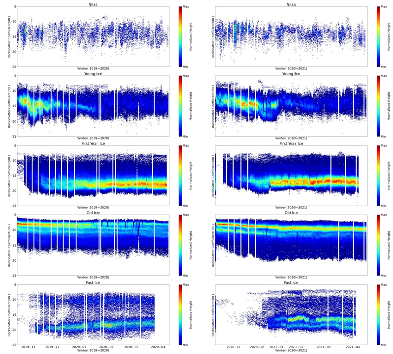
To illustrate the features of σ⁰ characteristics for MYI and FYI, the daily average ${\mathsf{\sigma }}^0$ histograms were stitched together and normalized to form σ⁰ time series plots. The σ⁰ under VV polarization time series plot demonstrates the seasonal variation of MYI and FYI. In Figure 2, the left and right columns are 2019/2020 and 2020/2021, respectively, and from top to bottom Nilas, YI, FYI, Old Ice, and Fast Ice are presented. The white area indicates absence of data. Days with insufficient data were removed.

Figure 2 shows that the distribution of the σ⁰ of Nilas was more heterogeneous. The σ⁰ of YI was between –12 and –15 dB in mid-October, and the reading gradually decreased to near –15 dB by the end of December due to freezing inside the sea ice. At this point, the number of Young Ice points was low due to the formation of FYI (thicker than 200 cm). From mid-October to mid-November, the σ⁰ of FYI remains unstable, because the Young Ice has not yet frozen into FYI. In mid-November, FYI starts to form, and its values are basically distributed between –15 and –20 dB. Due to the stable internal structure of MYI, σ⁰ was always between –6.5 and –10 dB, which is relatively easy to distinguish. The σ⁰ of Fast Ice exhibits a bimodal distribution, with a high σ⁰ located near the northern Canadian Archipelago and low values located near the Kara Sea, which must be distinguished by another parameter. 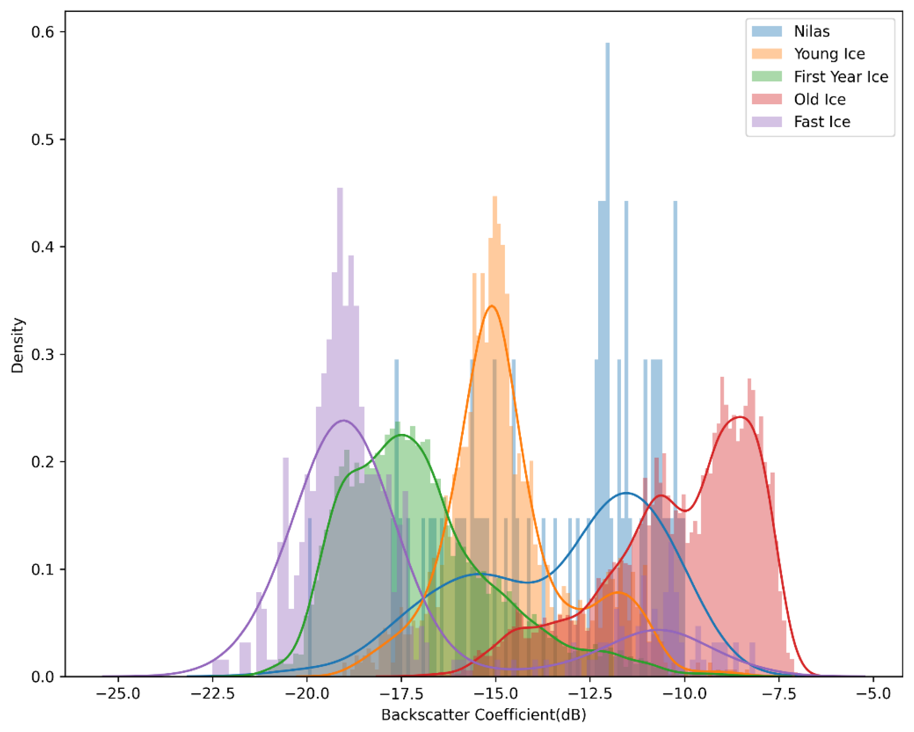Figure 3 shows the density distribution diagram of each ice type on 1 January 2020, and the density distribution of each ice type on a single day also conforms to the above conditions.

By analyzing time series histograms and monthly mean values of σ⁰ of each ice type, the values of σ⁰ of Young Ice, FYI, and Old Ice were found to be significantly different under VV polarization. In addition, Nilas and Fast Ice are significantly different from other ice types after introducing the polarization gradient ratio, and they can be distinguished by a nonlinear classifier.

3.2.2. Analysis of Monthly Mean σ⁰

In comparison to FYI, there are more bubbles inside MYI [35]; therefore, the penetration depth of the scatterometer pulse is deeper in MYI than in newly formed ice, and the strong volume scattering leads to a higher σ⁰ in MYI than in FYI [36]. At the same time, the salinity of MYI is lower than that of FYI, resulting in deeper penetration of MYI. Furthermore, the salinity of FYI is higher than that of MYI, leading it to possess stronger electromagnetic absorption properties [4]. Hence, the σ⁰, as well as the polarization ratio, can be used as a basis for sea ice classification.

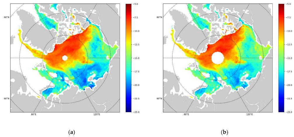
Figure 4 shows the distribution of monthly average σ⁰ for different ice types under VV polarization and HH polarization for a total of 16 months from October 2019 to April 2020 and from October 2020 to April 2021. From the distribution, the monthly average σ⁰ scattering values of Fast Ice and FYI are similar, and other parameters must be introduced to distinguish them. The values of YI are in the range of –15 to –13 dB due to the early stage of sea ice formation, and the range of values is close to Nilas, which can be distinguished using features such as the polarization gradient ratio.

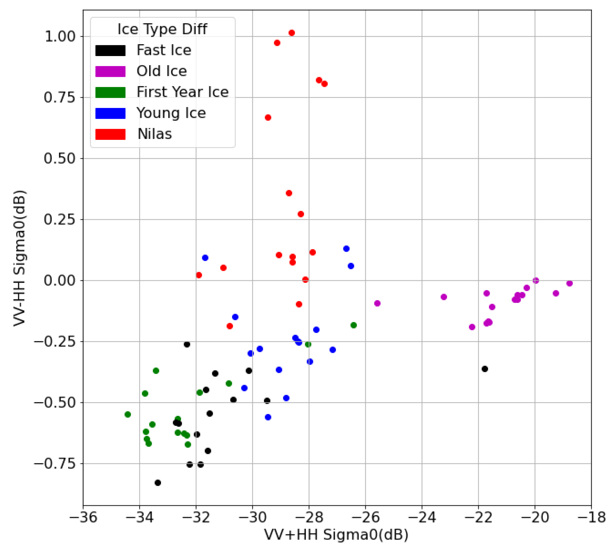
The difference between the signals of each polarization is more apparent in Figure 5. As a resulot of the high surface salinity of Nilas, the value of ${\mathsf{\sigma }}_{\mathrm{VV}}^0$ − ${\mathsf{\sigma }}_{\mathrm{HH}}^0$ is generally higher than zero. When Nilas gradually thickens and forms Young Ice (between 10 and 30 cm), ${\mathsf{\sigma }}_{\mathrm{VV}}^0$ − ${\mathsf{\sigma }}_{\mathrm{HH}}^0$ starts to decrease, whereas the value of ${\mathsf{\sigma }}_{\mathrm{VV}}^0$ + ${\mathsf{\sigma }}_{\mathrm{HH}}^0$ remains between –30 and –26 dB, similar to Nilas. The polarization ratio of the σ⁰ of FYI is similar to that of the Fast Ice distribution area, but the value of ${\mathsf{\sigma }}_{\mathrm{VV}}^0$ + ${\mathsf{\sigma }}_{\mathrm{HH}}^0$ is somewhat higher compared to that of Fast Ice. The parameter distribution characteristics of Old Ice are significantly different from other ice types; the value of ${\mathsf{\sigma }}_{\mathrm{VV}}^0$ + ${\mathsf{\sigma }}_{\mathrm{HH}}^0$ is distributed between –26 and –18 dB and the value of ${\mathsf{\sigma }}_{\mathrm{VV}}^0$ − ${\mathsf{\sigma }}_{\mathrm{HH}}^0$ is above 0 dB. The ${\mathsf{\sigma }}_{\mathrm{VV}}^0$ + ${\mathsf{\sigma }}_{\mathrm{HH}}^0$ of Fast Ice is generally distributed between –30 and –32 dB, which is significantly different from FYI. We conclude that the polarization ratio (PR) and the gradient ratio (GR) can be used for sea ice classification. PR and GR can be calculated using Equations (2) and (3), respectively.

$$\mathrm{PR}={\sigma }_{VV}^0/{\sigma }_{HH}^0$$

(2)

$$\mathrm{GR}={\sigma }_{VV}^0-{\sigma }_{HH}^0/{\sigma }_{VV}^0+{\sigma }_{HH}^0$$

(3)

3.3. DT Classification

We first attempted a preliminary classification of sea ice types for FYI-MYI using the threshold method of σ⁰, and the classification results were used as one of the input parameters of the DT. Subsequently, an attempt to refine the sea ice classification was made using various combinations of parameters. By adding parameters such as the dynamic threshold pre-classification of FYI-MYI values, PR, and GR to the machine learning model, the classification performance of the model can be improved.

3.3.1. Pre-Classification by ${\mathsf{\sigma }}^0$ Threshold

To provide an effective MYI and FYI broad class (including Nilas, Young Ice, and FYI) of segmentation features for machine learning models, those two classes can be separated by setting a threshold value. The ice type of fast ice is more specific; in the Kara and Laptev Seas there is FYI, and in Canadian Arctic Archipelago there is MYI; therefore, the fast ice data does not contain this broad classification feature. Haarpaintner [36], in 2007, used a threshold of –12 dB to segment MYI and FYI. Physical properties such as surface roughness, salinity, and thickness of multi-year and FYI change daily, resulting in variations in σ⁰ observations [35]; therefore, segmenting ice species using only a fixed σ⁰ threshold would result in errors. In this study, we used a dynamic threshold to classify ice as either FYI or MYI, which means that pixels with ${\mathsf{\sigma }}^0$ above the threshold are classified as MYI, while below the threshold, they are classified as FYI. An adaptive sea ice classification threshold was set to correspond to each histogram.

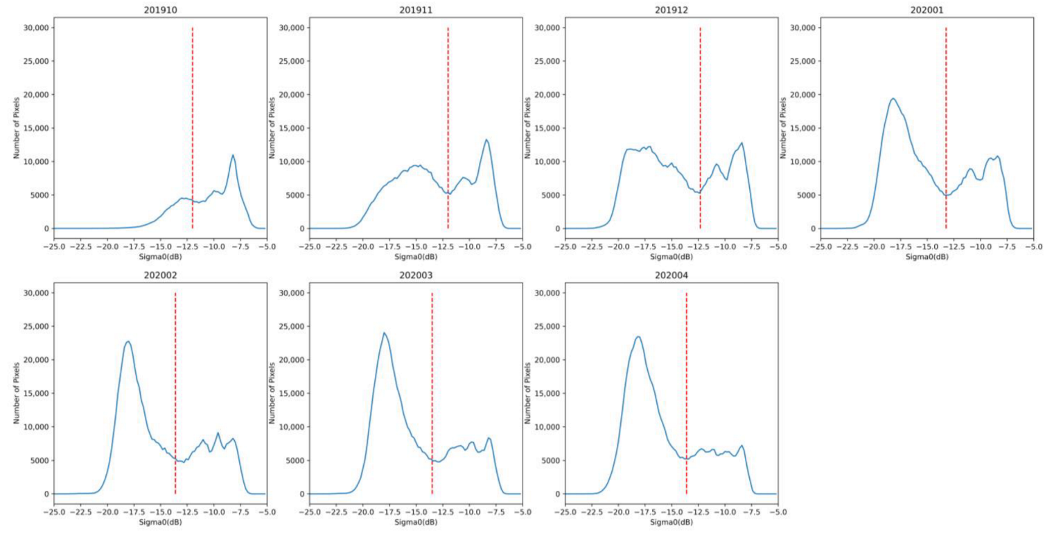
In the process, each HY-2B SCA monthly histogram was first plotted, and then for each histogram the lowest value between the bimodal peaks was adopted as the threshold for the month. Furthermore, the threshold was specified between –10 and –14 dB, and if there was no minimum between these values, a value of –12 dB was adopted. To reduce the error caused by histogram fluctuations, monthly histograms were used instead of daily histograms for sea ice classification.

Figure 6 shows the threshold from October to April 2019/2020.

3.3.2. Parameter Selection

The largest influence on the accuracy of the DT is from the selection of input features. Furthermore, due to the seasonal variation in the characteristics of ice types, which is shown in Figure 1, time is also used as an input parameter in different forms, such as the month, week, and day of the year (DOY). Five different combinations of temporal and backward scattering coefficient dimensional features were used as training data. Data from October 2019 to April 2020 and October 2020 to April 2021, with a total of 8,339,334 points, were collected and divided into training and test sets at a ratio of 7:3. One day per month was selected not to participate in the training process for validation. The accuracies obtained are shown in

Table 1. Classification accuracy for each parameter of decision tree.

Parameters	Overall Accuracy
${\sigma }_{VV}^0$, Month, FYI-MYI-PRE	91.75%
${\sigma }_{VV}^0$, DOY, FYI-MYI-PRE	96.06%
${\sigma }_{VV}^0$, Week, FYI-MYI-PRE	94.25%
${\sigma }_{VV}^0$, Week	94.22%
Week, ${\sigma }_{VV}^0$ + ${\sigma }_{HH}^0$, ${\sigma }_{VV}^0$ − ${\sigma }_{HH}^0$	93.94%

. FYI-MYI-PRE indicates the pre-classification parameter by the threshold.

In the course of the experiment, we took one day out of each month of the training set to observe the classification performance of each feature combination. After a comprehensive comparison of the classification accuracy and regional classification performance, (${\sigma }_{VV}^0$, week) and (${\sigma }_{VV}^0$, DOY, pre-classification) were finally selected as the two sets of feature values.

3.4. Image Segmentation Method

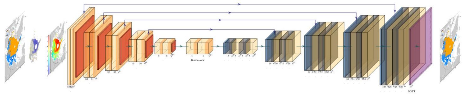
In this section, a tuned U-Net, consisting of an encoder (for downsampling) and a decoder (for upsampling) [33] was employed. Images of Arctic sea ice features were fed to the U-Net network, encoded by downsampling to obtain a set of features smaller than the original image, and then subsequently decoded by an upsampler to reduce the original image size and obtain a map of the classification results of the original image. This image segmentation network is then trained by back propagating the differences between the results obtained and the real segmentation, which was from the AARI Ice Chart in this research. The theoretical significance of downsampling is to increase the robustness of some small perturbations of the input image, reduce the risk of overfitting, reduce the number of operations, and increase the size of the perceptual field. The role of upsampling is to restore the image features extracted by downsampling to the initial pixel size and finally obtain the segmentation result. In the recovery process of the up-sampled image, the information is supplemented and the convergence speed is increased by skip connection to prevent the information loss caused by the change in feature scale [37].

To improve the robustness of the model and reduce the number of trainable parameters, a MovileNetV2 pre-trained model was used as the feature extraction model in this study, and the intermediate output values of this model were used as the input values in the U-Net network to improve the training speed of the model. The network structure is shown in Figure 7.

${\sigma }_{VV}^0$, ${\sigma }_{HH}^0$, and ${\sigma }_{VV}^0$ + ${\sigma }_{HH}^0$/${\sigma }_{VV}^0$ − ${\sigma }_{HH}^0$ for a projected resolution of 25 × 25 km were used in a 128 × 128 × 3 image input model according to the RGB channel, and the categories were set as Nilas, YI, FYI, MYI, and Fast Ice.

3.5. Model Fusion

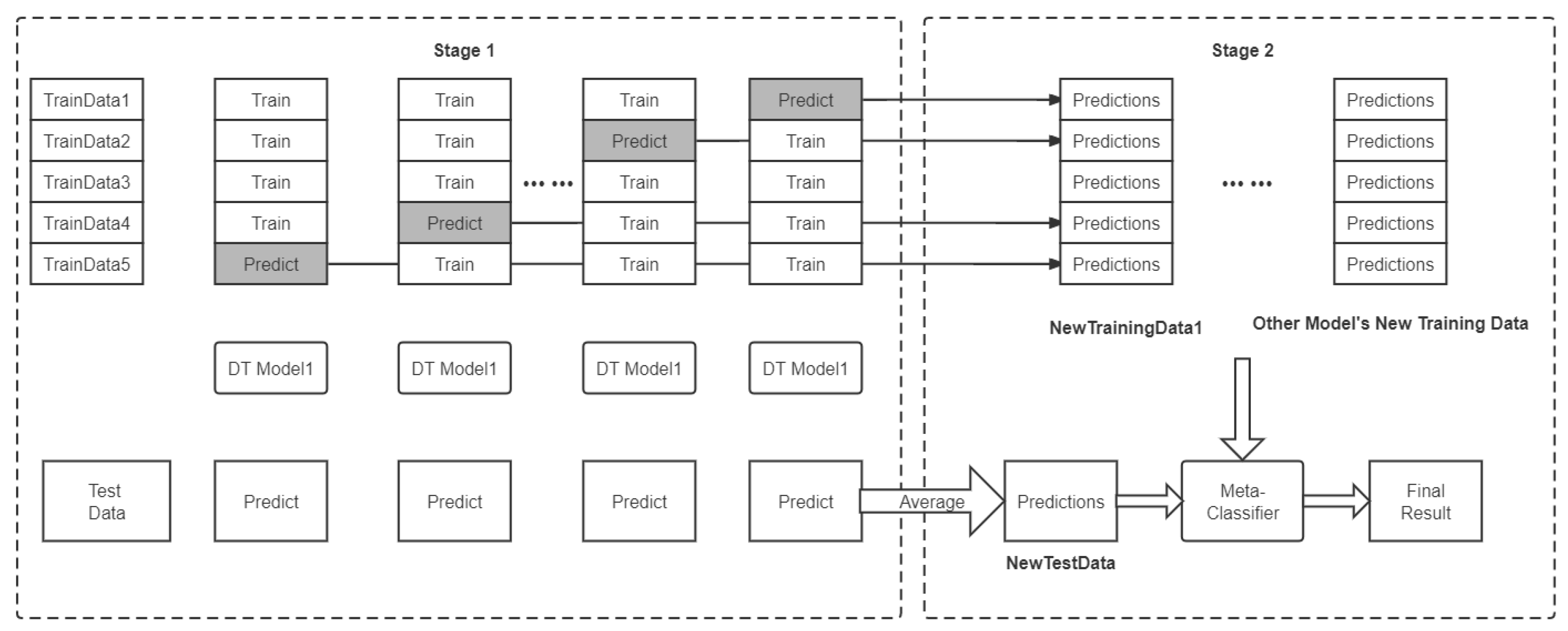
The core idea of the stacking model approach is to generate a meta-model. This meta-model is generated by using a k-Fold cross-validation technique on the prediction results of one set of machine learning sub-models (i.e., weak learners) as the training set, and using an additional simple model to train to obtain the final strong learner. In this study, the two previously mentioned DT models with different features and an image segmentation model were used as sub-learners for model fusion.

Table 2. Selection of sub-model parameters used for fusion.

Sub-Method\Feature	Backscatter Coefficient	Time	FYI-MYI-PRE	${\mathit{\sigma }}_{\mathit{V}\mathit{V}}^0$$/{\mathit{\sigma }}_{\mathit{H}\mathit{H}}^0$	${\mathit{\sigma }}_{\mathit{V}\mathit{V}}^0$$-{\mathit{\sigma }}_{\mathit{H}\mathit{H}}^0$$/{\mathit{\sigma }}_{\mathit{V}\mathit{V}}^0$$+ {\mathit{\sigma }}_{\mathit{H}\mathit{H}}^0$
Decision tree 1	${\sigma }_{VV}^0$	Week	×	×	×
Decision tree 2	${\sigma }_{VV}^0$	DOY	√	×	×
Image Segmentation	${\sigma }_{VV}^0,{\sigma }_{HH}^0$	×	×	√	√

shows the training parameters used for each sub-learner, and the results of the first-level training set by five-fold cross-validation.

Figure 8 shows the stacking model process. “√” mark means that the feature is used by the current submodel, and “×” means that it is not used. Parameters of daily average ${\mathsf{\sigma }}^0$, time, and the pre-classification result were first used as the initial training data, which were divided into training and test sets at a ratio of 5:1, and the training data set was cross-validated using five-fold cross-validation. Then, one-fifth of the training set was adopted as the sub-test set, while the other four-fifths were taken as the sub-training set to train the same model five times and make predictions for each sub-test set that are then stitched together with other sub-test set results to make the training set for Stage 2. At the same time, the classification results of the five test sets were averaged and used as the test set for Stage 2. This process was applied to DT model 1, DT model 2, and the image segmentation method to generate the corresponding data and test sets. The final fusion model was trained with a simpler structured DT model.

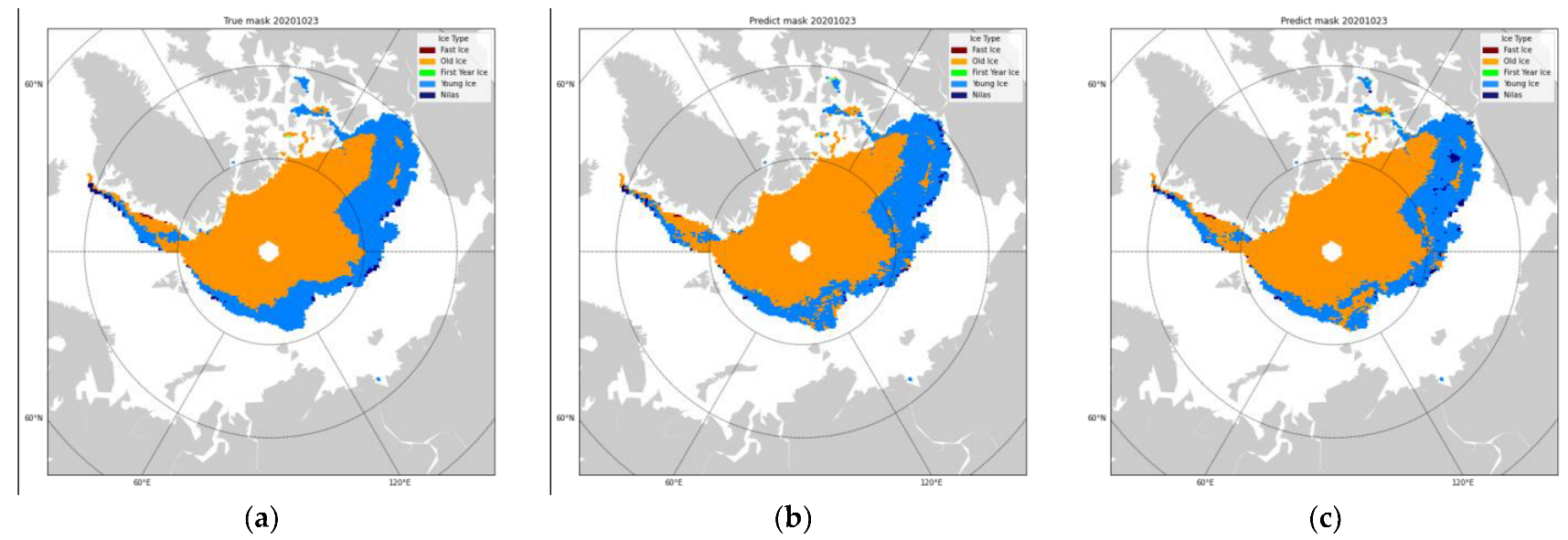
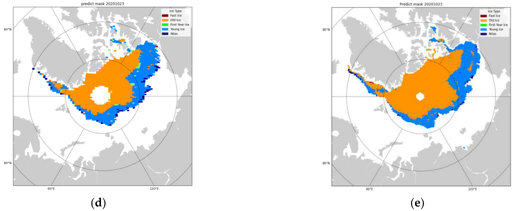
Figure 9 shows the classification results of each algorithm, taking 23 October 2020 as an example.

The missing data in the central region of the Arctic in Figure 9d is due to ${\sigma }_{HH}^0$ data used by the algorithm, which are not available in the region. Figure 9b,c shows that the DT model has good classification performance for the main part of the MYI, but there is a region where some YI was misclassified as Old Ice between 100°E and 120°E. Furthermore, the image segmentation model has good classification performance in this region, but there is some YI that was misclassified as FYI at the sea ice edge. After fusion, the classification performance was improved in the misclassified region for these three sub-models. This demonstrates that the stacking model fusion algorithm can be an effective alternative to traditional image-level algorithms for the correction task.

3.6. Sea Ice Classification Maps

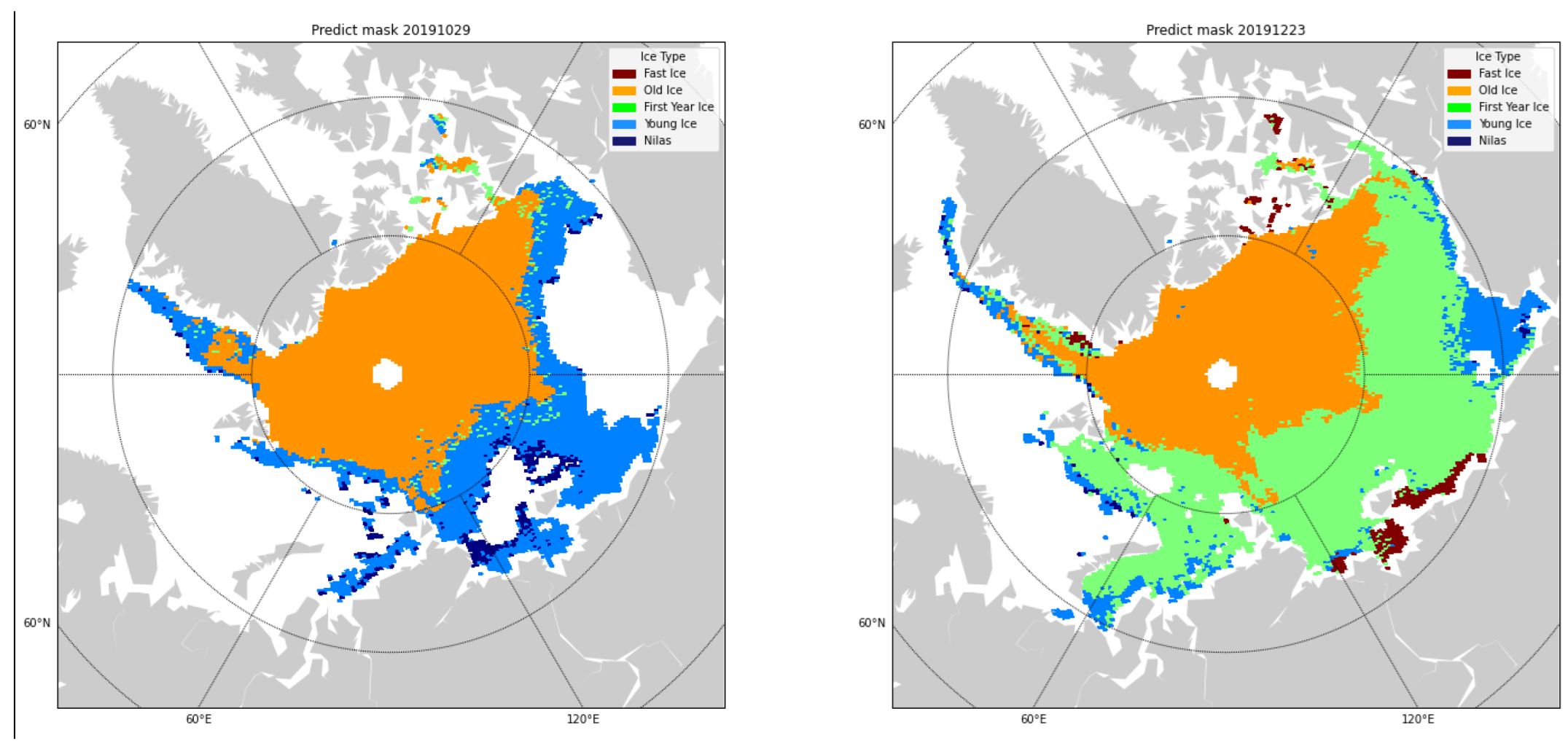
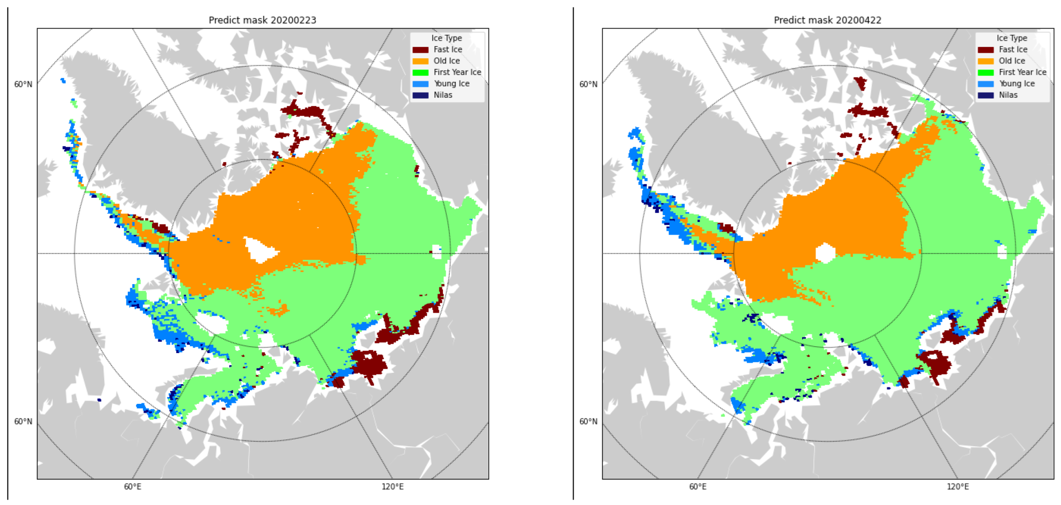
The HY2B SCA sea ice classification results for 2019/2020, 2020/2021, and 2021/2022 were obtained by the stacking model fusion algorithm, referred to in the following as stacking-HY2B. Figure 10 shows the prediction results on four days: 29 October 2019, 23 December 2019, 23 February 2020, and 22 April 2020.

We calculated the confusion matrix for the entire winter season using data from October 2021 to April 2022 as a validation, and the results are shown in

Table 3. Comparison of classification results with AARI in October 2021 to April 2022.

Classification Result		AARI					Accuracy
	Nilas	Young Ice	FYI	Old Ice	Fast Ice	Total
Nilas	19,927	4935	1974	1070	447	28,353	70.3%
Young Ice	4682	327,792	75,304	9896	4212	421,886	77.7%
FYI	3589	67,996	1,395,491	59,337	12,161	1,538,574	90.7%
Old Ice	687	39,828	106,710	1,427,211	1441	1,575,877	90.6%
Fast Ice	371	5214	30,343	3177	81,005	120,110	67.4%
Total	29,256	445,765	1,609,822	1,500,691	99,266	3,684,800

. A total of 3,684,800 points were counted. The largest errors were for Nilas, YI, and Fast Ice. The accuracy of Nilas was 70.3%, while some of the points of Nilas were incorrectly classified as Young Ice. The accuracy of Young Ice was 77.7%, and nearly 18% of the points (75,304) were misclassified as FYI, which is due in part becuase young ice is similar to FYI in physical characteristics during the freezing process. For Fast Ice, the user accuracy was 67.4%, because there is a regional difference in Fast Ice in some parts of the Arctic, e.g., in the Kara and Laptev Seas, Fast Ice is FYI.

4. Comparison and Discussion

Most current sea ice classification datasets only distinguish FYI and MYI; therefore, there are no multiple sea ice classification methods or long-time and large-scale in situ data to verify the classification results. In this study, we used the OSI-SAF sea ice type dataset as the comparison data, and areas with large classification differences were subsequently assessed using EASE-GRID Sea Ice Age data. As a result of the lack of on-site actual measurement data, the CMEMS data and EM-Bird ice thickness measurements were selected as the validation data.

4.1. Comparison with OSI-SAF Sea Ice Type

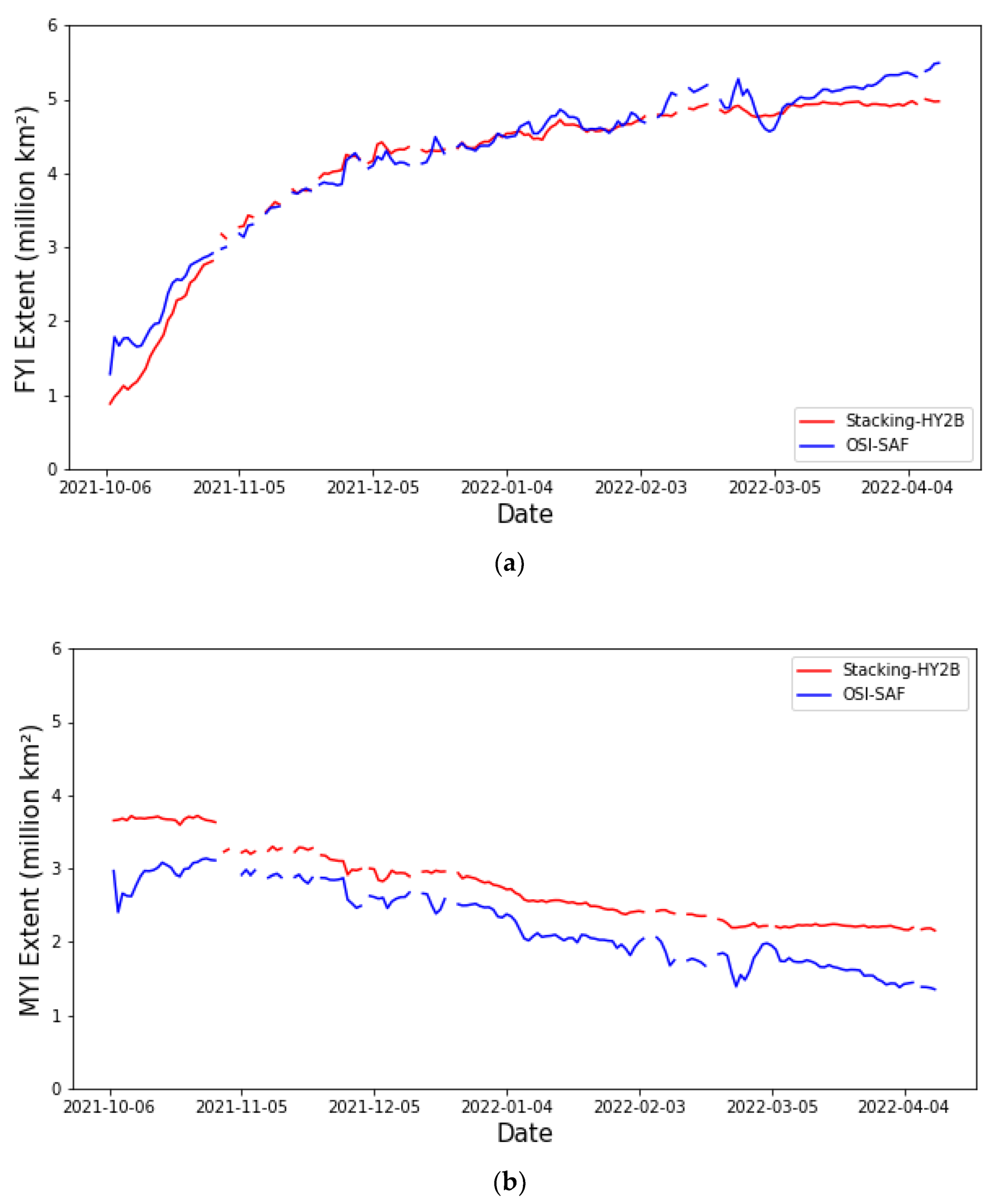
First, we compared the sea ice extent of the two data sets, as shown in Figure 11, from October 2021 to April 2022. The sea ice extent was obtained by summing the area of each pixel point to calculate the total, removing the days with incomplete satellite data. OSI-SAF data only distinguishes FYI and MYI; therefore, the Nilas, Young Ice, and First Year Ice from Stacking-HY2B were classified as FYI and Old Ice was classified as MYI. Since Fast Ice is one-year-old ice in areas such as the Kara and Laptev Seas in the Arctic and MYI in the Canadian Arctic Archipelago, the areas classified as Fast Ice were not counted. Pixel points marked as ambiguous in the OSI-SAF data were not included in the calculation.

Figure 11a indicates that the results of the Stacking-HY2B and OSI-SAF have a basically consistent trend in both FYI and MYI, which changes with the season. In winter, the area of FYI in Stacking-HY2B gradually increases from the lowest value of $0.91\times {10}^6 {\mathrm{km}}^2$ in October to $5.01\times {10}^6 {\mathrm{km}}^2$ in April.

In Figure 11b, there is a certain difference in the area of extent between the two data sets of MYI, and the average classification result difference in sea ice extent is $0.53\times {10}^6 {\mathrm{km}}^2$. The difference in the extent of MYI is smaller from November 2021 to December 2021 and larger from February 2022 to March 2022. The maximum MYI extent for Stacking-HY2B is $3.71\times {10}^6 {\mathrm{km}}^2$, and for OSI-SAF is $3.13\times {10}^6 {\mathrm{km}}^2$. This indicates that the MYI extent decreases, while the FYI extent increases.

Table 4. Confusion matrix results on 2021/2022 data comparison with OSI-SAF.

Classification Result	OSI-SAF			User Accuracy
	FYI	MYI	Total
FYI	1,386,345	144,989	1,531,334	90.53%
MYI	48,439	736,374	784,813	93.82%
Total	1,434,784	881,363	2,316,147
Overall Accuracy = 91.64%

shows the confusion matrix between Stacking-HY2B and OSI-SAF.

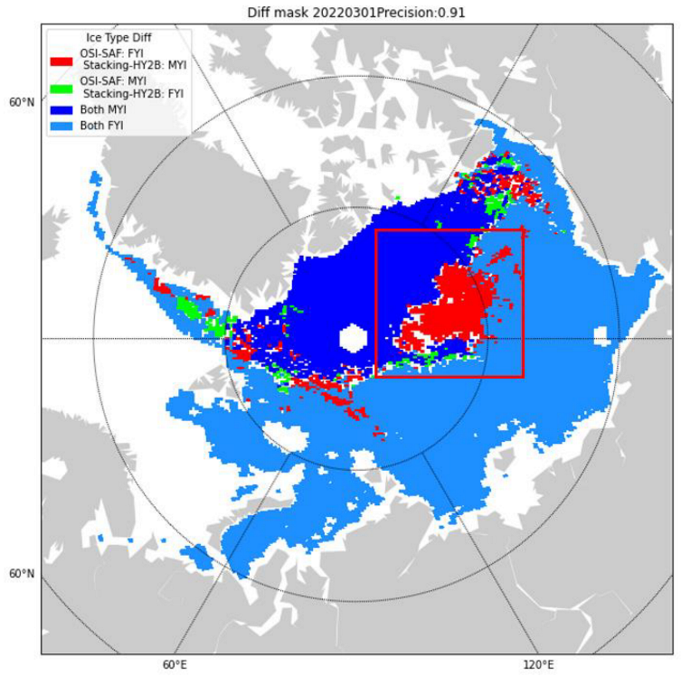
The overall accuracy was 91.64%, and the user accuracy of FYI and MYI was 90.53% and 93.82%, respectively. The areas where there is a difference are analyzed next. Taking 1 March 2022 as an example, Figure 12 shows the difference distribution of the two data sets to analyze MYI differences.

Figure 12 shows that the areas classified as FYI by OSI-SAF and MYI by Stacking-HY2B are mainly concentrated in the central Arctic (CA, Figure 12 boxed area). This indicates that Stacking-HY2B has a higher amount of MYI extent than OSI-SAF. For the area boxed in Figure 12, we selected sea ice age (SIA) data to compare the classification results, which classify the sea ice into 0–1-, 1–2-, 2–3-, and 3+-year-old ice in Figure 13.

This indicates that in the boxed area, the sea ice is more than one year old, which means that it is MYI. This is consistent with the inversion results of the Stacking-HY2B model.

4.2. Validation Using CMEMS Sea Ice Type Product

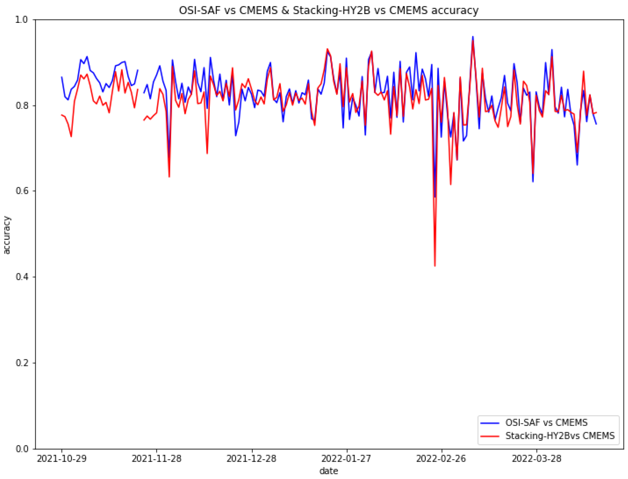
To further investigate the classification accuracy of Stacking-HY2B, we compared it to the CMEMS SAR-based sea ice type dataset. The accuracy evolution with time of Stacking-HY2B and OSI-SAF are shown in Figure 14. The accuracy is calculated by dividing the number of correctly identified pixel points by the total number of pixel points. According to time coverage of ${\mathsf{\sigma }}^0$, we used data from November 2021 to March 2022 for validation.

Figure 14 illustrates the recognition accuracy was between 0.87 and 0.92 for both types. The identification accuracy of OSI-SAF was higher than that of Stacking-HY2B by about 0.03 from October to December 2021, while their accuracy remained about the same in January 2022. This is because at the early stage of the formation of FYI, the DT model cannot effectively identify the characteristics of MYI, as the σ⁰ of ice types in some regions are not evident. The structure of newly formed FYI is relatively stable after December; therefore, the identification accuracy can be on par with the OSI-SAF product.

4.3. Validation Using EM-Bird Ice Thickness Measurements

Due to the lack of actual sea ice type data, we used the EM-Bird measurement data of sea ice thickness, extracted and projected into a 25 KM × 25 KM grid, and converted it into four sea ice typed (Nilas, Young Ice, FYI, and MYI) by the relationship between sea ice type and thickness [2]. To match the period of EM-Bird measurements, two freezing seasons from October 2020 to April 2021 and from October 2021 to April 2022 were used as training data in the validation process, and then 5 days of helicopter measurements from 4 April 2020, 10 April 2020, 17 April 2020, 26 April 2020, and 30 April 2020 were used to validate with the sea ice types obtained from the inversion. The spatial range of the comparison is 83.6°N–85.2°N and 6°E–20°E, and the results of the comparison are shown in

Table 5. Comparison accuracy over five days: EM-Bird vs. Stacking-HY2B.

Date	Matching Points	Number of FYI	Number of OI	Overall Accuracy
4 April 2020	24	5	19	79.16%
10 April 2020	4	0	4	100%
17 April 2020	3	0	3	100%
26 April 2020	10	0	10	100%
30 April 2020	2	0	2	100%

.

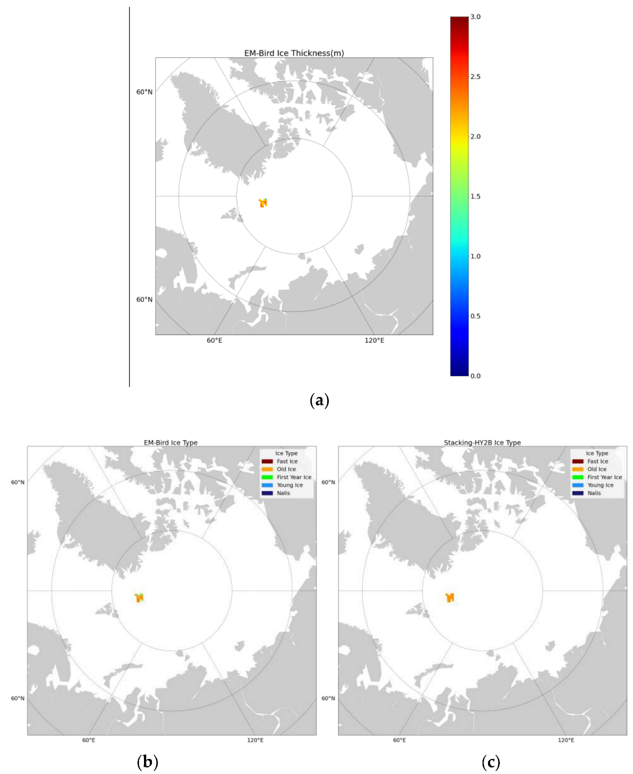
Due to seasonal and observational location limitations, EM-Bird only shows two types of ice: FYI and OI. The ice type pixel points obtained from the conversion of the airborne observations on all dates are consistent with the results of this study, except for 4 April 2020, when there is a comparison error of the points close to 20%. This research analyzed all data from the 4 April 2020, and Figure 15 shows the ice thickness of EM-Bird, the converted ice chart, and the inversion results of Stacking-HY2B at the corresponding positions.

It can be inferred that the difference in the comparison mainly comes from two aspects. The first is an ice thickness–ice conversion error. Due to the direct conversion of sea ice thickness to ice type in the WMO-IOC Technical Commission for Oceanography and Marine Meteorology SIGRID-3 format, there are some pixels with thickness around 1.8–2 m in the chart, and these pixels have been converted to 1-year-old ice, while in fact, they are most likely MYI. The second is that the spatial resolution of HY2B SCA is much coarser than EM-Bird.

4.4. Discussion

The difference in MYI between Stacking-HY2B and OSI-SAF in the CA regions may arise from several reasons: First, the different active microwave sensors have different sensitivities to sea ice types. The Ku band scatterometer employed by the Stacking-HY2B is more sensitive to the sea ice type than the C band ASCAT employed by OSI-SAF [20]. Second, it may be due to some changes in the prevailing ice thickness of one-year ice compared to the years developed in SIGRID-3 format. The classification results of the Stacking-HY2B are closer to that of SIA than OSI-SAF, possibly because the DT algorithm uses the threshold method for pre-classification, and the dynamic threshold can effectively differentiate ice types from FYI to MYI according to their trends.

In the validation process, the proximity posterior probability of each ice type in the classification model can cause inaccurate ice type determination. For example, within the sea ice pixel at the edge of FYI and MYI, the probability of FYI of this pixel in the classification algorithm is close to the probability of MYI because of the close microwave properties of sea ice. The classification result of this pixel may not be determined correctly in this case. In turn, this results in Stacking-HY2B detecting a lower density of MYI, inducing a loss in classification accuracy. Furthermore, due to the regional limitation of CMEMS data and EM-Bird ice thickness measurements, Stacking-HY2B cannot represent the retrieval accuracy of the whole Arctic. Further evaluation and validation of the algorithm using other high precision data will be attempted in the future.

5. Conclusions

Based on the HY-2B SCA data and the AARI ice maps, an innovative stacking model incorporating a DT algorithm and an image segmentation algorithm is used in this study to retrieve multiple sea ice types in the Arctic. Due to the use of dynamic threshold segmentation, this is not an operational algorithm.

First, the optimal features for the classification of multiple sea ice types are selected by comparing the sensitivity of σ⁰ to sea ice types. Six parameters are used in the study, they are satellite observed σ⁰ under VV and HH polarization (${\mathsf{\sigma }}_{\mathrm{VV}}^0,{\mathsf{\sigma }}_{\mathrm{HH}}^0$), σ⁰ ratio, σ⁰ polarization gradient ratio, DOY, and pre-classification features by the monthly histogram threshold method.

Second, we use stacking to fuse the three sub-models trained by the DT algorithm and image segmentation algorithm using different parameters. This successfully improves the performance of the filtering and masking compared to image correction after classification, which is commonly used in sea ice classification algorithms. This means that the performance is improved at the algorithm level, and beneficial recognition results are achieved by Stacking-HY2B.

Finally, Stacking-HY2B is compared with the OSI-SAF product. The results show that the extent of FYI in winter 2021/2022 is about the same, and the extent of MYI calculated by Stacking-HY2B is about $0.58\times {10}^6{\mathrm{m}}^2$ more than that of the OSI-SAF product. The difference in sea ice extent is mainly from differences in the Central Arctic. Additionally, we then introduced the EASE-Grid Sea Ice Age dataset to evaluate the classification differences in the Central Arctic sea region, and the Stacking-HY2B is found to be closer to the SIA dataset than the OSI-SAF dataset. Validation using the CMEMS product showed that Stacking-HY2B is comparable to the OSI-SAF product in terms of the classification accuracy, but the categories are more refined. The EM-Bird airborne measurements are also used to verify the sea ice classification results, with an overall accuracy of 88.37%, and the causes of the errors were analyzed. The classifier obtained by fused model using a stacking algorithm in this study is able to effectively distinguish Arctic sea ice types.

In future work, we will consider applying this classification method to other scatterometers and improving models so that they can be operational. If the incidence angle of the applied scatterometer is variable, we will perform an incidence angle correction first. At the same time, the current monthly dynamic threshold method of pre-classification can also be improved; we will consider adding dynamic ± X days thresholds to the classification. Additionally, the water content of snow on sea ice will likely affect the σ⁰; therefore, we will use air temperature data, such as ERA5, in the future to exclude areas with excessive water content.