


Vision-Based Dynamic Response Extraction and Modal Identification of Simple Structures Subject to Ambient Excitation


Abstract
:1. Introduction
2. Theoretical Background
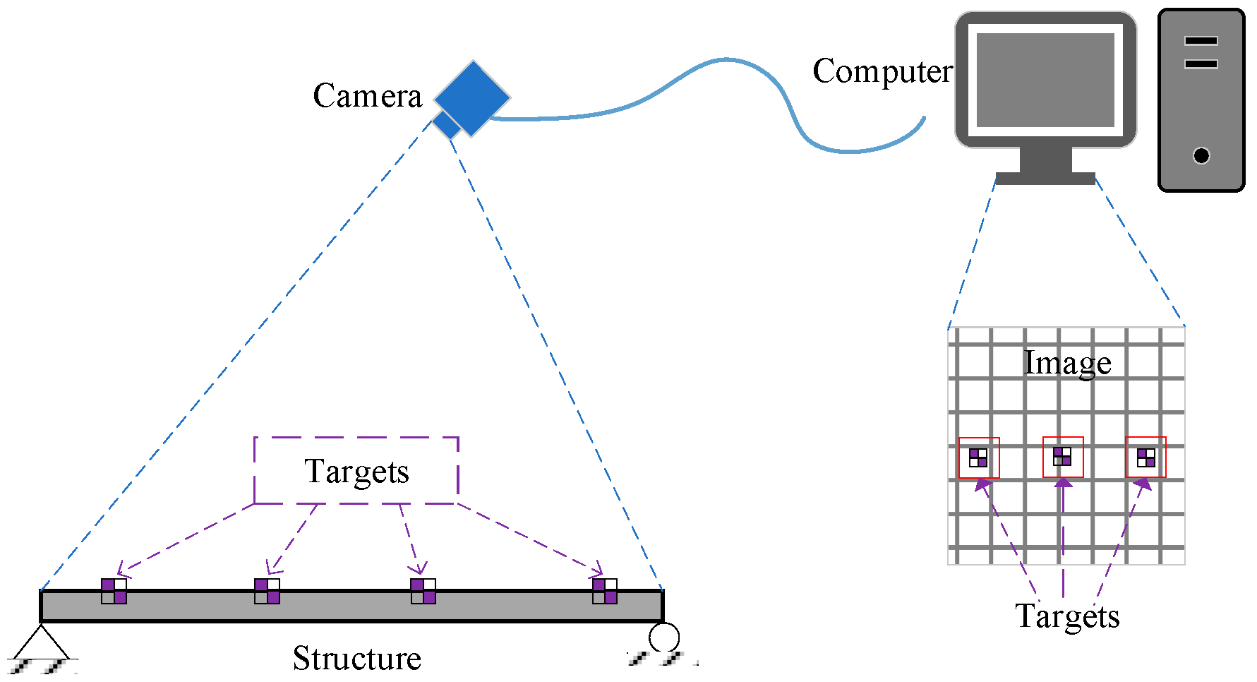
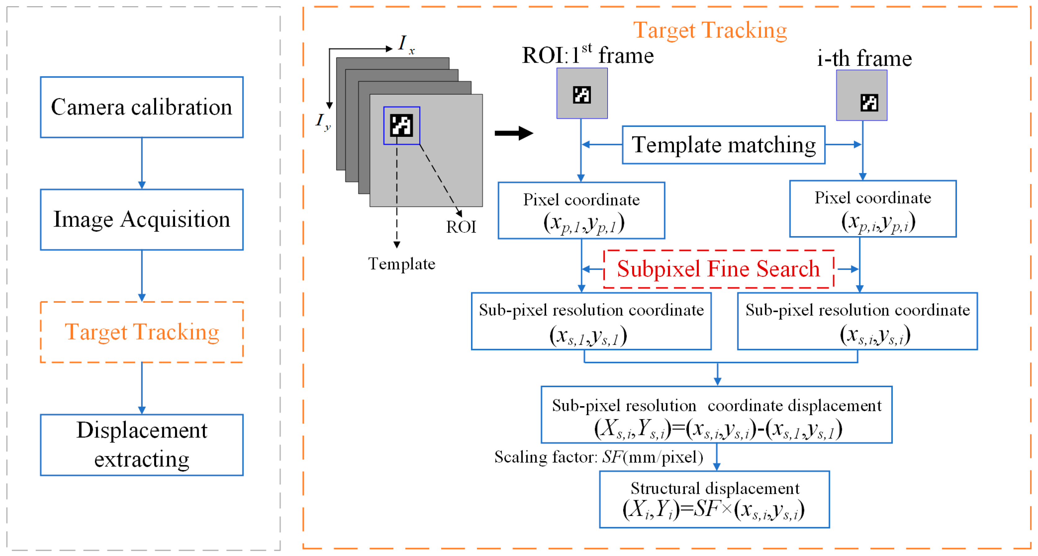
2.1. Dynamic Response Extraction Based on Template Matching at the Subpixel Level
2.2. Output-Only Modal Parameter Identification of Structures under Environmental Excitation
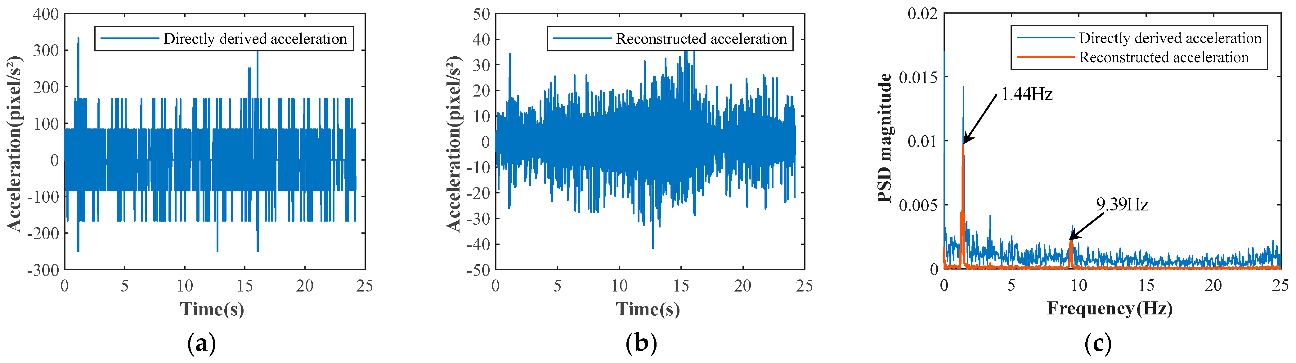
3. Proposed Signal Reconstruction Method
4. Experimental Study
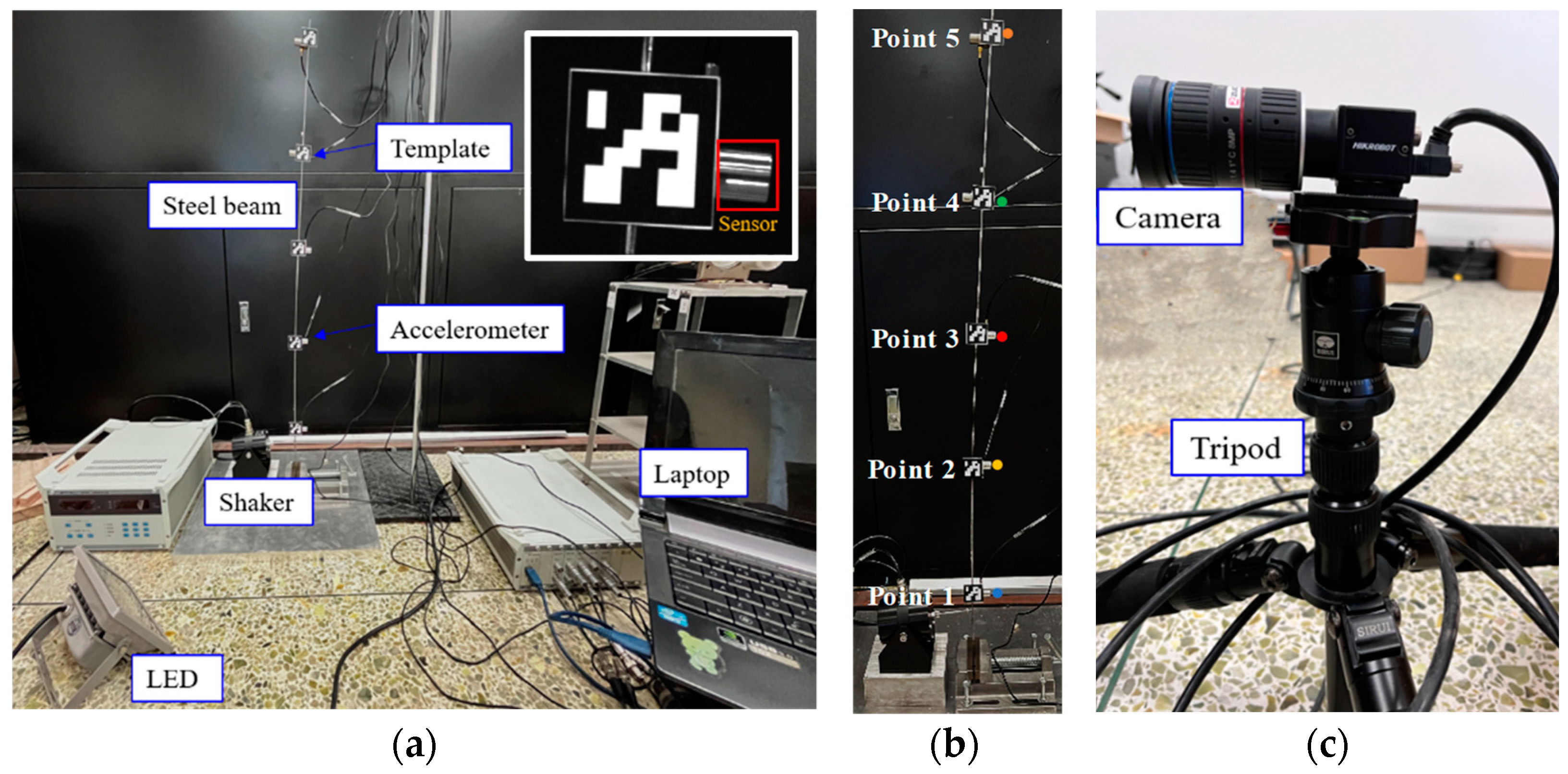
4.1. Experimental Design and Test Setup
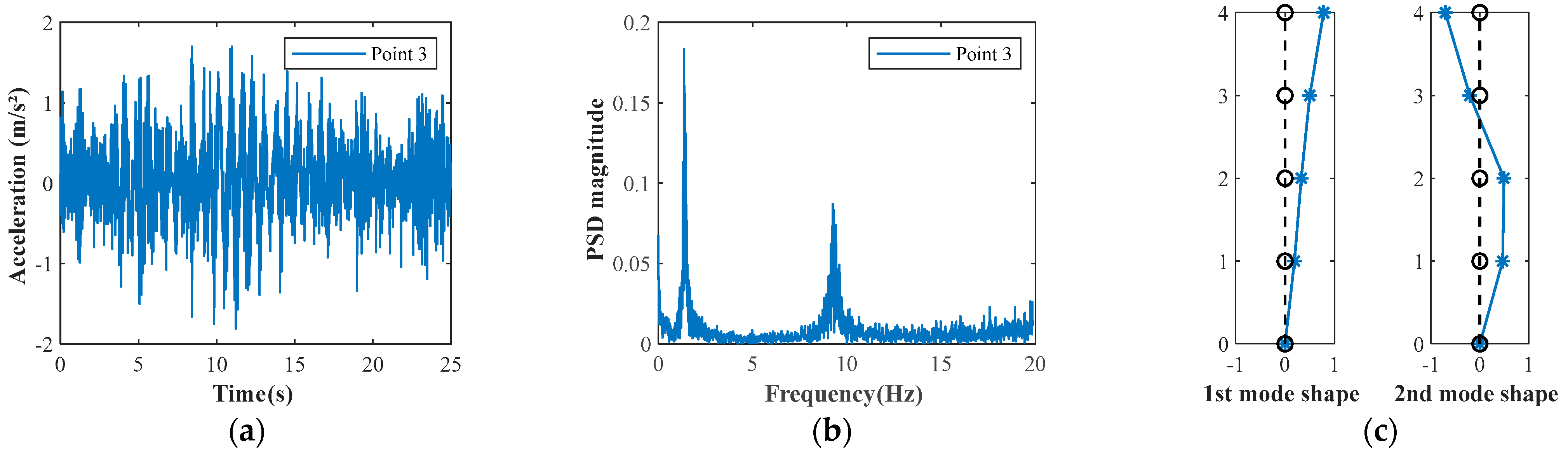
4.2. Modal Analysis by Acceleration Measurement
4.3. Mode Shape Identification by the Proposed Method
4.4. Effect of Camera Settings on the Proposed Method
5. Conclusions
- The proposed framework can identify the first two natural frequencies and mode shapes even if the vibration amplitude is as small as 0.01 mm, while the traditional vision-based method can only identify the modal parameters of the first two modes if the vibration amplitude is at least 0.06 mm.
- The proposed method performed quite well in the experimental test where three camera settings, including different focal lengths and object distances, were considered, indicating that it has great potential to be applied in various conditions. It should be noted that the proposed method is also applicable to other types of structure although only a cantilever beam was used for illustration in the experimental test.
- Preliminary experiments on cantilever steel beams were carried out in the laboratory in this study. However, due to the low sampling rate of the camera in comparison to the accelerometer, challenges remain in estimating higher mode frequencies and mode shapes. Moreover, in order to assure the high quality of vision-based dynamic responses, the templates or pre-labeled targets were used in the experimental test. Hence, future research should be conducted to eliminate the usage of pre-labeled targets to make vision-based approach more practical.
Author Contributions
Funding
Institutional Review Board Statement
Informed Consent Statement
Data Availability Statement
Conflicts of Interest
Nomenclature
| I(x,y) | source image | fs | sampling frequency |
| T(x,y) | template image | mode shape vector | |
| DFT | discrete Fourier transform | M | mass matrix |
| Ad | state matrix | C | damping matrix |
| Bd | input matrix | K | stiffness matrix |
| Cd | output matrix | ÿ(t) | acceleration vector |
| Dd | feed-through matrix | ẏ(t) | velocity vector |
| x(k) | state vector | y(t) | displacement vector |
| y(k) | measurement vector | F(·) | Fourier transform |
| u(k) | excitation vector | ωm | mth angular frequency |
| Hk | Hankel matrix | ŷ(t) | reconstructed displacement |
| fm | mth natural frequency | â(t) | the reconstructed acceleration |
References
- Qu, X.; Shu, B.; Ding, X.; Lu, Y.; Li, G.; Wang, L. Experimental study of accuracy of high-rate gnss in context of structural health monitoring. Remote Sens. 2022, 14, 4989. [Google Scholar] [CrossRef]
- Cai, Y.F.; Zhao, H.S.; Li, X.; Liu, Y.C. Effects of yawed inflow and blade-tower interaction on the aerodynamic and wake characteristics of a horizontal-axis wind turbine. Energy 2023, 264, 126246. [Google Scholar]
- Feng, D.; Feng, M.Q. Vision-based multipoint displacement measurement for structural health monitoring. Struct. Control Health Monit. 2016, 23, 876–890. [Google Scholar]
- Enshaeian, A.; Luan, L.; Belding, M.; Sun, H.; Rizzo, P. A contactless approach to monitor rail vibrations. Exp. Mech. 2021, 61, 705–718. [Google Scholar]
- Luan, L.; Zheng, J.; Wang, M.L.; Yang, Y.; Rizzo, P.; Sun, H. Extractingfull-field subppixel structural displacements from videos via deep learning. J. Sound Vib. 2021, 505, 116142. [Google Scholar]
- Toh, G.; Park, J. Review of vibration-based structural health monitoring using deep learning. Appl. Sci. 2020, 10, 1680. [Google Scholar] [CrossRef]
- Wang, Z.; Yang, D.H.; Yi, T.H.; Zhang, G.H.; Han, J.G. Eliminating environmental and operational effects on structural modal frequency: A comprehensive review. Struct. Control Health Monit. 2022, 29, e3073. [Google Scholar]
- Lu, Z.-R.; Lin, G.; Wang, L. Output-only modal parameter identification of structures by vision modal analysis. J. Sound Vib. 2021, 497, 115949. [Google Scholar]
- Feng, D.; Feng, M.Q.; Ozer, E.; Fukuda, Y. A vision-based sensor for noncontact structural displacement measurement. Sensors 2015, 15, 16557–16575. [Google Scholar] [CrossRef] [PubMed]
- Bruhn, A.; Weickert, J.; Schnörr, C. Lucas/Kanade meets Horn/Schunck: Combining local and global optic flow methods. Int. J. Comput. Vis. 2005, 61, 211–231. [Google Scholar] [CrossRef]
- Fleet, D.J.; Jepson, A.D. Computation of component image velocity from local phase information. Int. J. Comput. Vis. 1990, 5, 77–104. [Google Scholar]
- Zhang, D.; Fang, L.; Wei, Y.; Guo, J.; Tian, B. Structural low-level dynamic response analysis using deviations of idealized edge profiles and video acceleration magnification. Appl. Sci. 2019, 9, 712. [Google Scholar] [CrossRef]
- Yang, Y.; Dorn, C.; Mancini, T.; Talken, Z.; Kenyon, G.; Farrar, C.; Mascareñas, D. Blind identification of full-field vibration modes from video measurements with phase-based video motion magnification. Mech. Syst. Signal Process. 2017, 85, 567–590. [Google Scholar]
- Javh, J.; Slavič, J.; Boltežar, M. High frequency modal identification on noisy high-speed camera data. Mech. Syst. Signal Process. 2018, 98, 344–351. [Google Scholar] [CrossRef]
- Bregar, T.; Zaletelj, K.; Čepon, G.; Slavič, J.; Boltežar, M. Full-field FRF estimation from noisy high-speed-camera data using a dynamic substructuring approach. Mech. Syst. Signal Process. 2021, 150, 107263. [Google Scholar]


| Output Voltage of Excitation (mV) | Displacement | Power Spectral Density (PSD) |
|---|---|---|
| 300 |  |  |
| 600 |  | 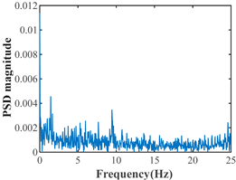 |
| 900 |  | 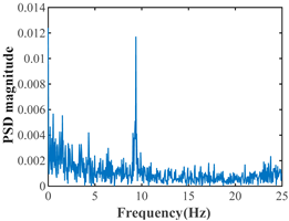 |
| 1200 | 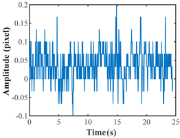 |  |
| 1500 | 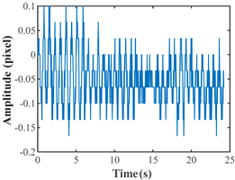 |  |
| Output Voltage of Excitation (mV) | Original Disp. | Directly Calculated Acc. | Reconstructed Acc. | |||
|---|---|---|---|---|---|---|
| 300 | —— | —— | —— | —— |  | 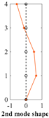 |
| 600 | —— | —— | —— | —— |  | 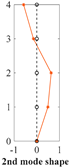 |
| 900 | —— | 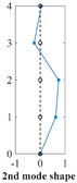 | —— |  |  | 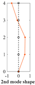 |
| 1200 | 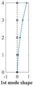 |  | —— |  | 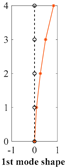 | 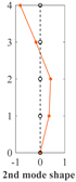 |
| 1500 | 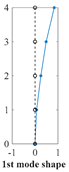 |  | —— |  | 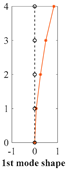 |  |
| Camera Setting | Original Disp. | Directly Calculated Acc. | Reconstructed Acc. | |||
|---|---|---|---|---|---|---|
| f = 12 mm u = 160 cm | —— | —— | —— | —— |  | 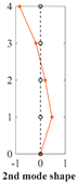 |
| f = 12 mm u = 200 cm | —— | —— | —— | —— | 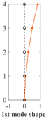 |  |
| f = 35 mm u = 200 cm | 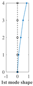 | 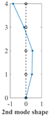 | —— | —— |  | 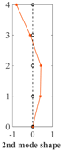 |
Disclaimer/Publisher’s Note: The statements, opinions and data contained in all publications are solely those of the individual author(s) and contributor(s) and not of MDPI and/or the editor(s). MDPI and/or the editor(s) disclaim responsibility for any injury to people or property resulting from any ideas, methods, instructions or products referred to in the content. |
© 2023 by the authors. Licensee MDPI, Basel, Switzerland. This article is an open access article distributed under the terms and conditions of the Creative Commons Attribution (CC BY) license (https://creativecommons.org/licenses/by/4.0/).
Share and Cite
Chen, Z.; Ruan, X.; Zhang, Y. Vision-Based Dynamic Response Extraction and Modal Identification of Simple Structures Subject to Ambient Excitation. Remote Sens. 2023, 15, 962. https://doi.org/10.3390/rs15040962
Chen Z, Ruan X, Zhang Y. Vision-Based Dynamic Response Extraction and Modal Identification of Simple Structures Subject to Ambient Excitation. Remote Sensing. 2023; 15(4):962. https://doi.org/10.3390/rs15040962
Chicago/Turabian StyleChen, Zhiwei, Xuzhi Ruan, and Yao Zhang. 2023. "Vision-Based Dynamic Response Extraction and Modal Identification of Simple Structures Subject to Ambient Excitation" Remote Sensing 15, no. 4: 962. https://doi.org/10.3390/rs15040962
APA StyleChen, Z., Ruan, X., & Zhang, Y. (2023). Vision-Based Dynamic Response Extraction and Modal Identification of Simple Structures Subject to Ambient Excitation. Remote Sensing, 15(4), 962. https://doi.org/10.3390/rs15040962