Impact of a Tropical Cyclone on Terrestrial Inputs and Bio-Optical Properties in Princess Charlotte Bay (Great Barrier Reef Lagoon)

Abstract

In January 2013, tropical cyclone Oswald caused widespread flooding in the North-East coast of Australia, and large and highly episodic inputs into Princess Charlotte Bay (PCB, northern Great Barrier Reef). Freshwater outflows from the Normanby and Kennedy rivers, the two main rivers draining the adjacent catchments, resulted in drastic changes in physical, biogeochemical and optical properties within PCB. On 31 January, 2 days after the peak riverine discharge from the Normanby river, nutrients and dissolved organic matter contents peaked under the influence of large outflows from the Kennedy river into the western section of the bay (5.8 μM for dissolved inorganic nitrogen, 6.9 g m⁻³ for dissolved organic carbon and 6.1 m⁻¹ for the colored dissolved organic matter absorption coefficient at 412 nm). In the eastern section of the bay, the situation appeared more ‘mixed’, with a suspended solids concentration reaching 23.1 g m⁻³ close to the Normanby river mouth. The main phytoplankton bloom occurred in the transition zone between the Kennedy and Normanby flood plumes, and was dominated by diatoms with a chlorophyll a concentration reaching 14.6 mg m⁻³. This study highlights the need to better describe the critical spatial and temporal scales of variability of key biogeochemical and optical properties after a major flood event. The data collected is key to improve the accuracy of ocean color remote sensing algorithms and regional biogeochemical budgets following highly episodic inputs.

1. Introduction

The coastal ocean plays a major role in global carbon cycling and budgets, and is under increasing anthropogenic pressures [1]. In recent years, the increase in the frequency of extreme climatic and meteorological events has led to flood events worldwide [2,3]. Rivers and floodplains are key to many socioeconomic activities and extreme flood events lead to lasting damage to infrastructure and marine coastal resources. The resulting riverine inputs have a major impact on biogeochemical functioning in the coastal zone, from reduction of the light available for vulnerable pelagic and benthic ecosystems (e.g., phytoplankton, seagrass and reef ecosystems) to changes in species composition and inputs of contaminants (e.g., [4,5,6,7,8]). The occurrence of more frequent extreme events resulting in widespread floods thus calls for a better quantification of their impact on particulate and dissolved inputs, the processing of these inputs in the estuarine and coastal zones, and the flow-on effects on ecosystems (from phytoplankton communities to fisheries). The critical time scales involved are key to estimate the short-term impacts and long-term trends in coastal ecosystems. Flood events in tropical and subtropical systems are highly episodic and mainly occur during the wet season. They are the result of intense rain events and can be initiated with the passage of tropical cyclones. The intensity of extreme precipitation is predicted to increase as a result of climate change [9] and references therein). The impact of extreme events on coastal biogeochemical cycling has been poorly studied globally due to their very nature (sporadic events) and the inherent logistical and safety limitations of targeted field sampling programs (e.g., [4,5,6,7,10].

In the World Heritage listed Great Barrier Reef (GBR) lagoon, flood plumes can extend up to 100 km into offshore waters and have lasting impacts on coastal ecosystems. Increased catchment runoff and decline in riverine water quality is a major threat to the interconnected complexity of coral reefs and seagrass ecosystems [11,12,13,14,15,16,17]. The GBR is the world’s largest coral reef ecosystem, with over 3000 individual reefs, and has recently been in the spotlight due to an increase in coral bleaching events [18]. Sediment and nutrient loads discharged into the inner GBR have increased by about 5 times since European settlement [19,20] and can be particularly damaging to the health of seagrass meadows and coral reefs [21,22]. The impacts of rain events associated with tropical cyclones are particularly hard to quantify, while they account for a large fraction of sediment and nutrient inputs. Several programs are in place to better quantify terrestrial inputs from the major rivers flowing into the GBR lagoon, and ambitious sediment and nutrient reduction targets have been set under the GBR Reef 2050 plan. In 2005, the Great Barrier Reef Marine Park Authority (GBRMPA) established the Marine Monitoring Program to monitor inshore water quality and coral reef and seagrass meadow health [23]. More recently, eReefs, a collaborative program using the latest technologies to collate data with integrated modelling, developed a coupled hydrodynamic, sediment, biogeochemical and optical model to provide near real-time critical information over the GBR lagoon and to undertake scenarios to inform management interventions (https://ereefs.org.au, last accessed on 10 October 2022, [12,24].

As part of a collaborative project between CSIRO (Commonwealth Scientific, Industrial and Research Organisation) and James Cook University, an intensive in situ sampling program was conducted during the entire 2012–2013 wet season across far-north Queensland (from the Burdekin river to Cape York, Figure 1—inset; [25], to examine terrestrial inputs into the coastal zone during flood events and for the calibration/validation of ocean color remote sensing algorithms and integrated models such as eReefs [15,25,26,27,28,29,30]. The present study in Princess Charlotte Bay (PCB), a remote coastal bay in North-East Australia, was part of a more extensive field campaign conducted between 26 January and 4 February 2013 in the mid to northern GBR [25]. Our field sampling coincided with the major riverine inputs into PCB following tropical cyclone Oswald, a low intensity (category 1) but high impact storm which made landfall over Northern Australia on 21 January 2013 [31]. Its passage caused storms, heavy rain, widespread flooding and catastrophic infrastructure and property damage over a 7-day period. Princess Charlotte Bay is a relatively pristine region of the GBR and the site of diverse and healthy marine coastal ecosystems. The adjacent catchments (Normanby and Kennedy basins) have particular economic, social and cultural values (land of the Bakanambia and Jeteneru people). The Normanby-Kennedy estuaries are the largest estuarine system in the GBR, and a major source of sediments, dissolved organic material and nutrients to the northern GBR lagoon [32,33]. The northern GBR estuaries have been mostly poorly studied due to logistical limitations associated with their remote location [32,33].

The in situ biogeochemical and optical datasets collected were used in combination with ocean color satellite imagery to examine the biogeochemical inputs and transformation processes within PCB, the impact on the phytoplankton community and the implications for remote sensing bio-optical algorithms during flood events. Bio-optical properties are key parameters in ocean color remote sensing algorithms to derive in situ biogeochemical properties. The fortuitous timing of the sampling allowed us to constrain the short-term variability, a critical scale in highly dynamic coastal systems. In turn, the satellite images provided a synoptic view of the situation pre- and post-floods in PCB. The increased frequency of extreme weather events around the world calls for a better quantification of their short-term and long-term impacts and the capability of coastal ecosystems for recovery [5,6,10]. The present study addresses some of the challenges involved in studying the impact of tropical cyclones on the unique coastal ecosystem that is the northern GBR and the major factors driving the fate of flood inputs in the coastal zone.

2. Materials and Methods

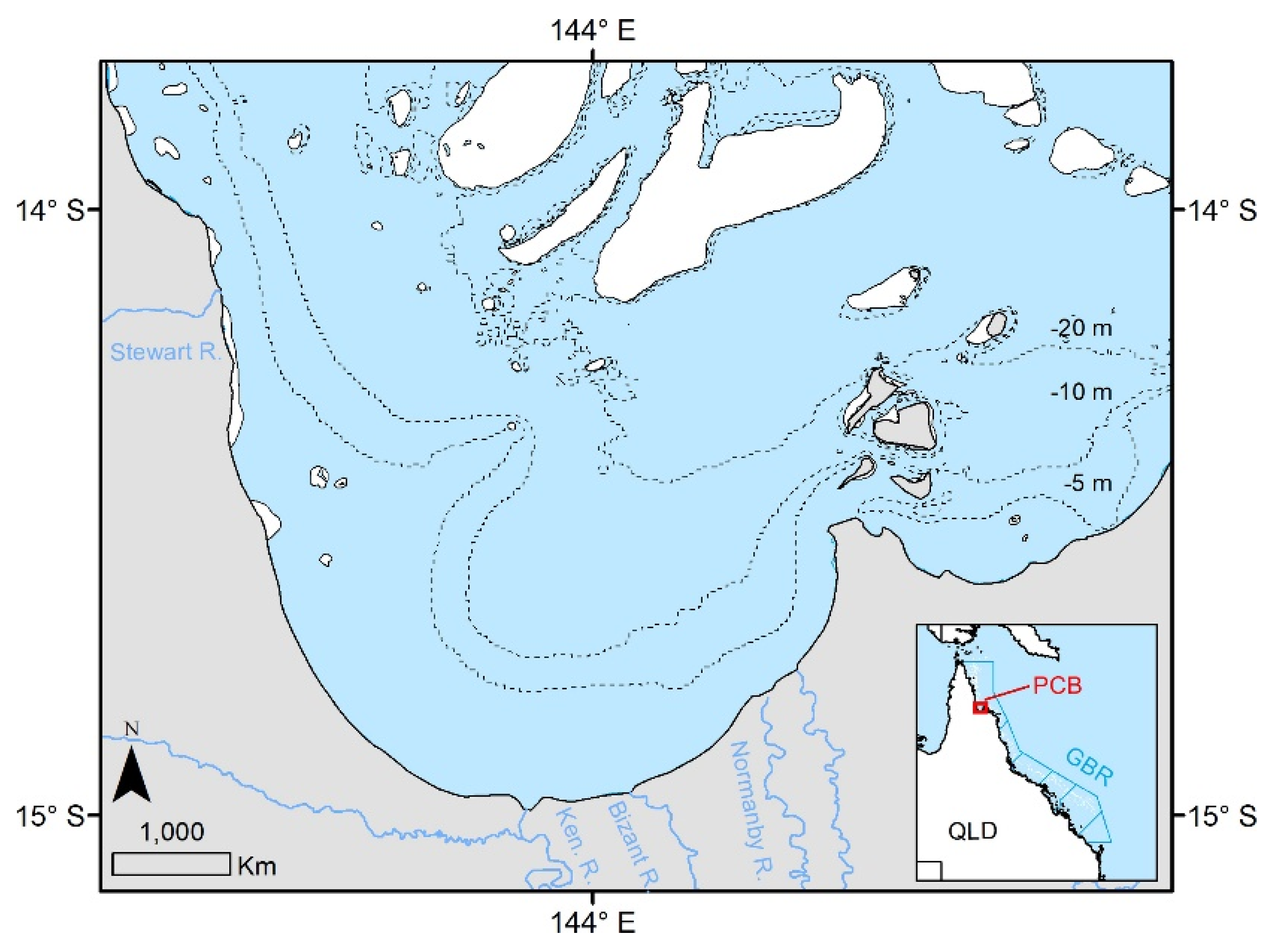
2.1. Study Area and Field Sampling

Princess Charlotte Bay (PCB) is a large shallow bay in remote North-East Australia (average depth of ~8 m), covering an area of 2000 km² (Figure 1). Within the GBR lagoon, PCB is a region of diverse and healthy marine and coastal habitats, from seagrass meadows, mangroves and salt flats to several coral reef ecosystems to the north. Three main rivers discharge into PCB: the North Kennedy, Bizant, and Normanby. The Normanby river is the fourth largest river system flowing into the GBR lagoon, and its catchment is the source of half of the sediment and nutrient inputs to the northern GBR [34,35]. Changes in land use since European settlement more than doubled the sediments and nutrients loads from the Normanby catchment [23] and references therein). The Bizant river is a smaller tributary which drains the adjacent salt flats during the wet season and can connect the North Kennedy and Normanby estuaries [33]. While the Normanby estuary is characterized by a narrow channel, the North Kennedy estuary (hereafter referred to as ‘Kennedy’) is associated with a wide shallow channel. Both the Normanby and Kennedy lower estuaries are bordered by extensive salt flats and fringing mangroves, while the upper tidal reaches are characterized by mangrove swamps. The adjacent catchments are semi-arid with a low population density (~500 residents), low-density but extensive cattle grazing, and large conservation areas in the Rinyirru and Jack Rivers National Parks. They are also home to many sacred aboriginal sites of the Bakanambia and Jeteneru people. Marine plains are also considered to be of high conservation value [32].

Riverine discharge occurs during the wet season (January to April) with 95% of the annual rainfall associated with episodic floods. Cyclones are known to occur on average every 2 years in the region [33]. The Normanby river is the only river with a gauging station located at Kalpowar Crossing (105107A), 77 km upstream from the river mouth. This gauging station is not representative of the wider Normanby basin discharge, but provides comparative information between wet seasons. Following tropical cyclone Oswald, rainfall in the PCB catchment was intense and the Normanby river rose to 8 m above baseline levels on 27 January. The flood peak reached PCB on 29 January (approximately 36 h later, therefore 1 day before the start of our field sampling on 30 January 2013). Total river discharge was equivalent to 860 GL over 19 days (Figure 2). The average flushing time during the wet season is 1 day [33]. Tides are semidiurnal with typically one dominant tide a day. During spring tides, maximum tidal current velocities can reach 1.0 and 2.1 m s⁻¹ in the Normanby and Kennedy basins, respectively, and the lower reaches of the estuaries can be inundated over several kms inland. A more detailed description of the region’s climatology can be found in [32].

The field sampling of PCB was conducted over a 3-day period, from 30 January to 1 February 2013. We sampled contrasted water types, from outer-shelf reef waters (blue oceanic waters) located North-East of PCB (st. 1081 and 1082), to turbid floodwaters from the Normanby and Kennedy rivers (e.g., st. 1083 to st. 1093) and clear blue waters in the north of PCB (e.g., st. 1095) (Figure 3). One station was sampled twice on 30 January and 1 February (st. 1084 and 1096, respectively). Tidal heights and current velocities were recorded overnight through the water column at 5 min intervals by a bottom mounted 1 MHz Aquadopp profiler (Nortek, Norway) acoustic profiler at 2 fixed stations in PCB, and showed maximal tidal current velocities in the range of 0.3–0.6 m s⁻¹. Wind conditions were dominated by strong northwesterly winds with an average a speed of 13 knots during our field sampling.

2.2. Discrete Biogeochemical Determinations

Total suspended matter (TSM): Sample water (0.5 to 3 L) was filtered through a 47 mm pre-weighed Whatman GF/F glass-fiber filter (muffled at 450 °C). The filter was then rinsed with ~50 mL of distilled water to remove any salt and dried to constant weight at 65 °C to determine the TSM concentration. The filters were placed in a muffle furnace at 450 °C for 3 h, allowed to cool and weighed to determine the amount of inorganic material remaining on the filter. The organic fraction was obtained by subtracting the inorganic fraction from the total TSM.

Phytoplankton pigments and phytoplankton size index: A given volume of sample water (0.1 to 3 L) was collected at the surface and filtered through a 47 mm Whatman GF/F glass-fiber filter and stored in a cryovial in liquid nitrogen until analysis. Pigments were extracted and analyzed by HPLC (High-Performance Liquid Chromatography) with a Waters-Alliance system (protocol described in detail in [36]. Total chlorophyll a (TChla) was calculated as the sum of monovinyl- and divinyl-chlorophyll a, and chlorophyll a allomers and epimers. Some pigments are specific to particular phytoplankton groups (e.g., peridinin in dinoflagellates, zeaxanthin in cyanobacteria) and referred to as ‘diagnostic pigments’ [37]), thus allowing us to derive the contribution of the different phytoplankton size classes [38,39]: microphytoplankton (size range: 20–200 μm), nanophytoplankton (2–20 μm) and picophytoplankton (0.2–2 μm).

Dissolved organic carbon (DOC), nutrients and salinity: For DOC, sample water was filtered through 0.45 μm syringe filters (Sartorius polyethersulfone) and the filtrate stored frozen until DOC determinations by High-Temperature Persulfate Oxidation using a 1010 TOC-Analyzer (OI Analytical) [40]. For nutrients, sample water was filtered through 0.45 μm syringe filters (Sartorius polyethersulfone) and the filtrate stored frozen until nutrient determinations using standard methods [41]. The protocols for nutrients and salinity analysis are described in more detail in [32].

Particulate absorption coefficient (phytoplankton and nonalgal): Sample water was collected at the surface ((0.1 to 3 L) and filtered through a 25 mm Whatman GF/F glass-fiber filter and stored flat in liquid nitrogen until analysis. The optical density of total particulate matter was measured over the 250–800 nm spectral range with 0.9 nm increments, using a Cintra 404 UV/VIS dual beam spectrophotometer equipped with an integrating sphere. Pigmented material was extracted from the sample filter using the method of [42] to determine the optical density of the nonalgal matter. The optical density due to phytoplankton was obtained by difference between the total particulate matter and the nonalgal particulate matter optical densities (over the full spectral range). Absorption coefficients were determined using the correction for the pathlength amplification of [43].

Colored dissolved organic matter absorption coefficient (CDOM): Sample water was filtered through a 0.22 μm filter (Millipore Durapore), and the filtrate stored in glass bottles and kept at 4 °C in the dark until analysis just after the field survey. The filtrate’s CDOM absorbance was measured from 250 to 800 nm in a 10 cm pathlength quartz cell using a Cintra 404 UV/VIS spectrophotometer, with fresh Milli-Q water as a reference. The absorption coefficient was normalized to zero at 680 nm. The spectral slopes S_275–295 and S_350–400 were produced by nonlinear least squares fitting of an exponential function to the CDOM absorption spectra over the corresponding wavelength ranges (275–295 nm and 350–400 nm, respectively). S_275–295 is a tracer of terrestrial dissolved organic carbon and an indicator of lignin content and photobleaching [44]. SR (unitless) was calculated from the spectral slopes ratio (S_275–295/S_350–400) [45].

2.3. In Situ Instrumentation

The diffuse attenuation coefficient of photosynthetically active radiation (K_d(PAR)) was obtained from depth profiles using a PAR sensor coupled with a CTD from Sea-Bird Electronics (SBE-19Plus), as described in [32]. In parallel, we deployed an instrument package comprising a WETLabs ac-s (absorption–attenuation meter) and a HOBILabs Hydroscat-6 (backscattering meter) in vertical profiling mode. An ac-s with a 10 cm pathlength was used for measurements of hyperspectral attenuation and absorption coefficients of total material (c(λ) and a(λ), dissolved plus particulate) between 400 and 730 nm, with a 4 nm resolution. Correction for in situ temperature and salinity effects on the optical properties of water was applied [46]. Incomplete recovery of the scattered light in the ac-s absorption tube was corrected for using the proportional method [47]. The ac-s was calibrated before the field campaign with optically pure Milli-Q water to quantify instrumental offsets. The backscattering coefficient was measured using the HOBILabs Hydroscat-6 [wavelengths: 442, 488, 555, 589, 676 and 852 nm]. A correction for incomplete recovery of backscattered light in highly attenuating waters (i.e., sigma correction [48] was applied using absorption and attenuation coefficients measured using the ac-s. The Hydroscat-6 was calibrated in the laboratory, prior to the field campaign, using the calibration device provided by HOBILabs: the signal response was measured through the sample volume (Milli-Q water) over a Lambertian reflective (Teflon) plaque [48].

3. Results

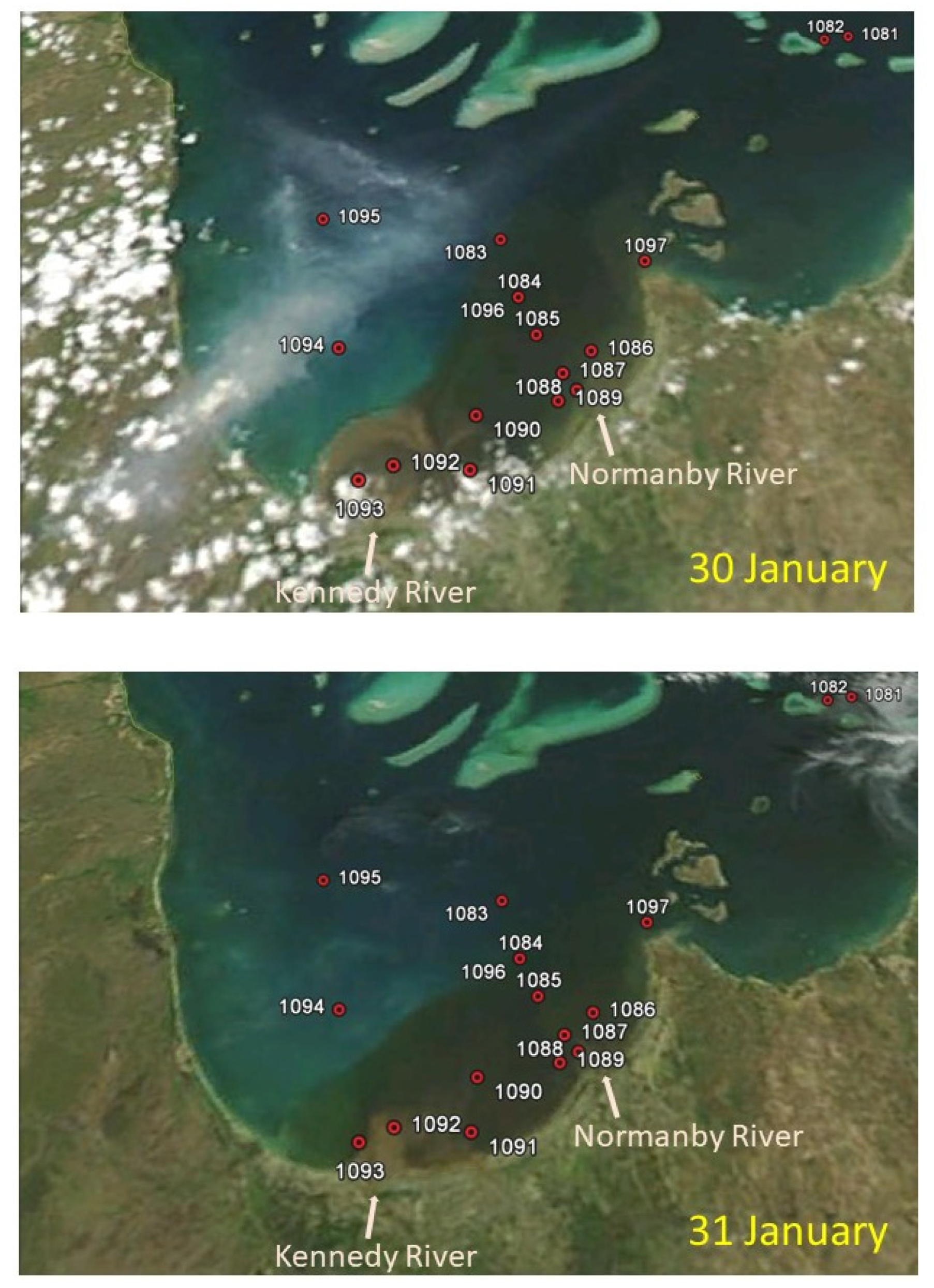
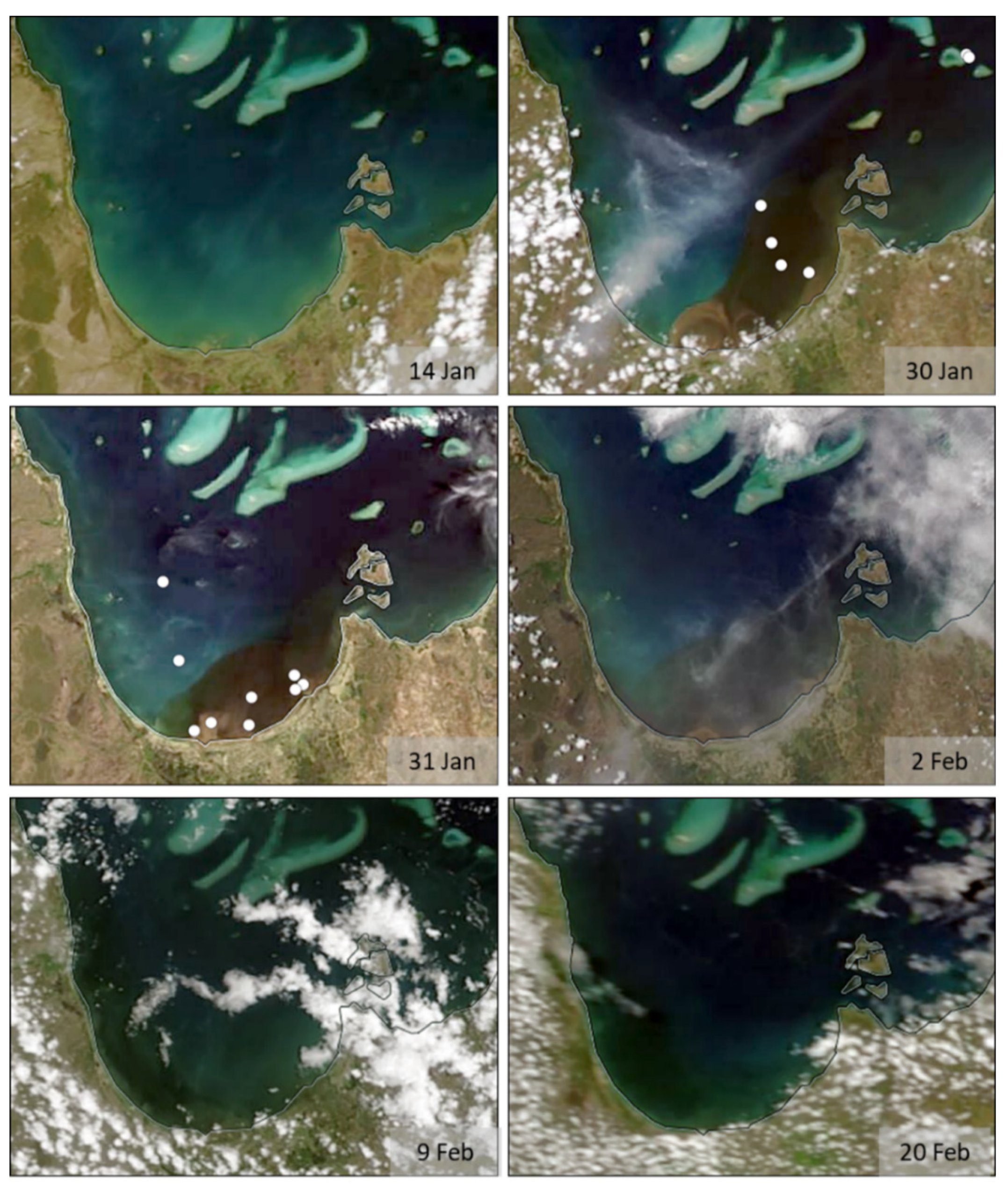
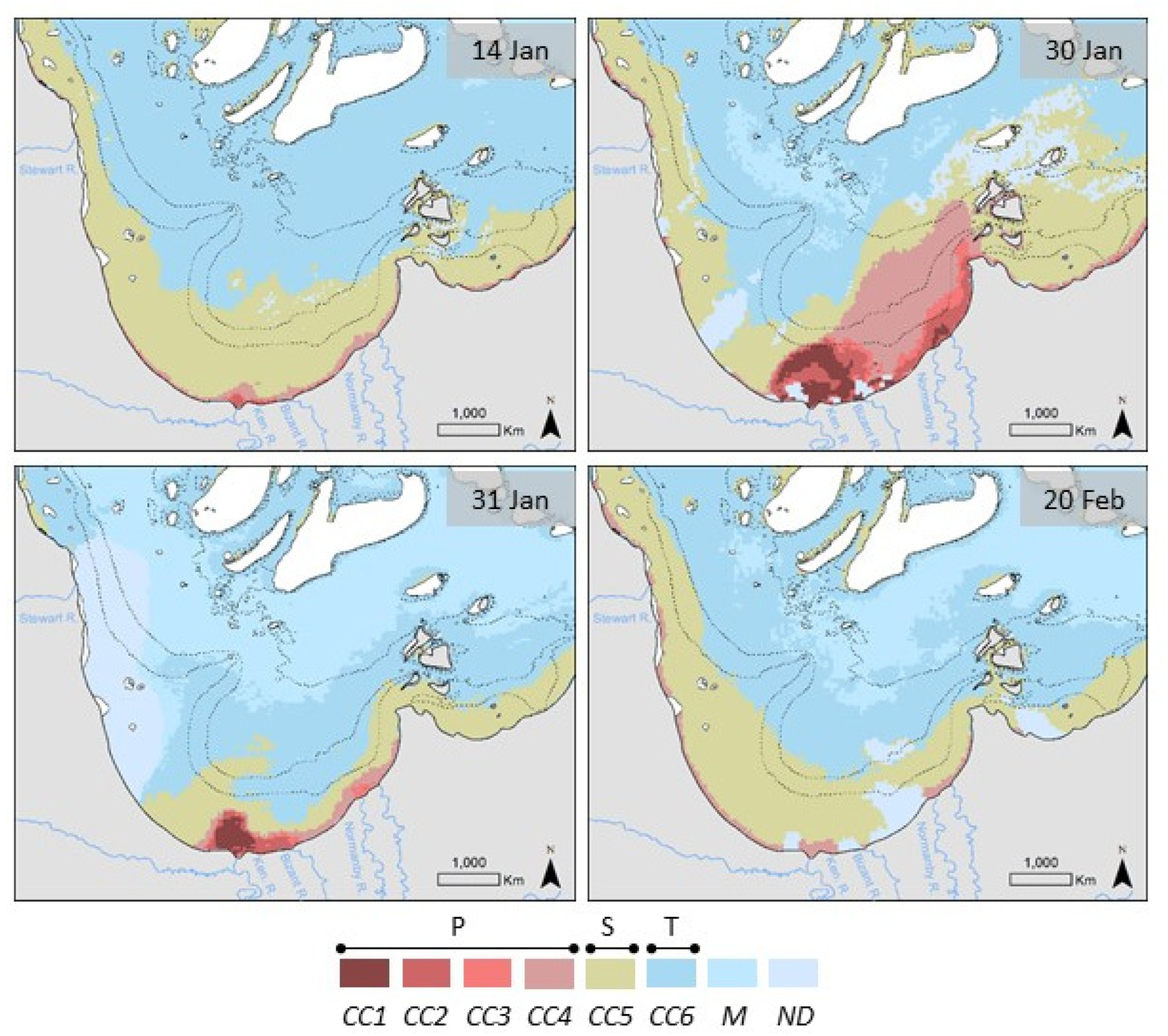
3.1. MODIS Ocean Color Maps

Time series of ocean color remote sensing RGB (red green blue) imagery (MODIS-Aqua and -Terra) demonstrates drastic changes in the optical and biogeochemical properties of surface waters after the passage of Tropical Cyclone Oswald (Figure 4). On 30 January (one day after the peak riverine discharge from the Normanby River), the extent of the flood plumes reached the midshelf reefs ~75 km to the east of PCB and covered an area of over 1400 km². Colored dissolved organic matter (CDOM) extended considerably further offshore than suspended solids (Figure 3, Figure 4 and Figure 5). The outflows from the Kennedy river were marked by a large and clearly delineated sediment-laden flood plume in the western section of the bay. A much smaller flood plume was also visible close to the mouth of the Bizant river. By contrast, the eastern section of the bay appears mostly dominated by CDOM except in the immediate vicinity of the Normanby river. Rapid return to baseline conditions occurred in the inshore regions on 09 February, with apparent return to near preflood conditions on 20 February.

The MODIS satellite images can be used to map reef optical water types. The full details on the methods used and associated uncertainties are given in [15,49]. Water types are classified depending on in situ water color and linked to water quality characteristics: primary waters (color class CC1-4) are brownish, enriched in sediment and dissolved organic matter, secondary waters (CC5) are greenish, usually enriched in dissolved organic matter and phytoplankton and with lower suspended sediment content, and tertiary waters (CC6) are clear and have low risk of detrimental ecological effects (Figure 5). Additionally marine waters correspond to offshore, clear waters and nondefined areas were not mapped due to interference or being outside of the study area.

The time-series of optical water types showed rapid changes following the peak riverine discharges into PCB (on 29 January for the Normanby river). On 30 January, maximum sediment inputs occurred in the western section of the bay (mostly CC1 to CC3), while the eastern section of the bay was dominated by CDOM (mostly CC4). From 30 to 31 January, the changes reached across several classes in inshore waters: from CC1 (sediments dominated) to CC5 (CDOM and phytoplankton dominated) in the western section of the bay, and from CC4 to CC5 in the eastern section of the bay. We had no access to satellite information prior to reaching PCB due to cloud cover (on 29 January). As a result, upon arrival on 30 January from the east, we started sampling the eastern section while maximum sediment inputs occurred in the western section (as shown by MODIS RGB imagery received later on that day). Despite not being able to measure the full range of variability postfloods due to these sampling limitations, we successfully described a large range of water types and some of the short time scale variability. It is important to highlight the need for better sampling strategies and the impact of the sampling chronology on in situ observations in this fast changing environment after major floods.

3.2. Physical Properties, Photosynthetically Active Radiation and Nutrients

Following the pulse of floodwaters into PCB, surface salinity dropped to ~17.0 and 3.4 near the Normanby and Kennedy mouths, respectively (st. 1089 and 1093) (

Table 1. Surface values for environmental and biogeochemical quantities at key stations in Princess Charlotte Bay. ‘n.a.’ denotes measurements were not available.

Station No. Region	1082 Outer-Reef	1087–1088–1089 Normanby R. Mouth	1092–1093 Kennedy R. Mouth	1095 North PCB	1084 (1096) Mid-Eastern PCB
Date	30 Jan.	31 Jan.	31 Jan.	31 Jan.	30 Jan. (1 Feb.)
Time	10:20	7:30–8:00–8:50	12:45–13:32	16:40	16:00 (10:10)
Salinity	n.a.	24.30–18.50–17.00	6.10–3.40	36.50	20.10 (35.30)
DIN (μM)	1.50	1.14–1.57–1.43	5.85–5.50	1.57	2.21–1.36
TSM (g m−3)	1.05	6.77–23.15–5.89	10.07–14.76	0.87	4.67 (0.84)
TSM Inorganic (%)	63.5	71.4–81.7–68.8	88.1–86.9	57.7	78.6 (69.7)
TChla (mg m−3)	2.97	6.38–5.86–11.15	0.90–1.20	0.20	5.74 (0.29)
DOC (g m−3)	0.92	3.32–5.39–4.56	6.00–6.88	0.98	3.82 (1.11)
aCDOM(440) (m−1)	0.02	1.88–3.32–3.42	3.46–3.81	0.14	2.07 (0.38)
aCDOM(412) (m−1)	0.04	2.95–5.26–5.14	5.53–6.09	0.19	3.20 (0.55)
SR (Slope Ratio)	3.12	0.88–0.87–0.95	0.86–0.85	2.92	0.96 (1.61)
aCDOM*(440) (m2 g−1)	0.026	0.56–0.62–0.75	0.58–0.55	0.15	0.54 (0.34)
bbp/bp(550) (%)	n.a.	1.9–4.7–1.5	3.3–n.a.	0.5	2.7 (n.a.)
b*(550) (m2 g−1)	0.60	0.87–0.23–n.a.	0.43–n.a.	1.05	0.43 (n.a.)
aCDOM/a(440) (%)	22.7	81.6–63.0–82.9	77.3–48.8	n.a.	81.4 (92.3)
aNAP/a(440) (%)	17.0	12.4–37.0–10.3	22.7–47.1	n.a.	12.5 (3.1)
aφ/a(440) (%)	60.3	6.0–0.0–6.7	0.0–4.1	n.a.	6.2 (4.6)

). Inshore waters were highly turbid, with Secchi depths of 0.30 and 0.85 m near the Normanby and Kennedy mouth, respectively. This is in agreement with the measured PAR diffuse attenuation coefficient (K_d(PAR)), with typically largest values near the Normanby mouth (1.92 m⁻¹ at st. 1089) and to a lesser extent near the Kennedy mouth (1.26 m⁻¹ at st. 1093). Floodwaters affected the whole water column with the most significant freshwater signature in the first 0.5 to 1.5 m (as derived from vertical profiles, data not shown). By contrast, the north of PCB was characterized by typically clear marine waters (surface salinity of 36.5 and Secchi depth of 6.75 m at st. 1095). Floodwaters lead to a high dissolved inorganic nitrogen concentration (DIN) near the Kennedy mouth (5.5 to 5.8 μM) and to a lesser extent near the Normanby mouth (1.1 to 1.6 μM). The repeat station (st. 1084 and 1096, Table 1) showed rapid changes in physicochemical properties and nutrient concentrations within 42 h: Secchi depth increased by a factor 6 (from 1.5 to 9.5 m), while DIN dropped by nearly a factor 2.

3.3. Biogeochemical Properties and High Frequency Bio-Optical Proxies

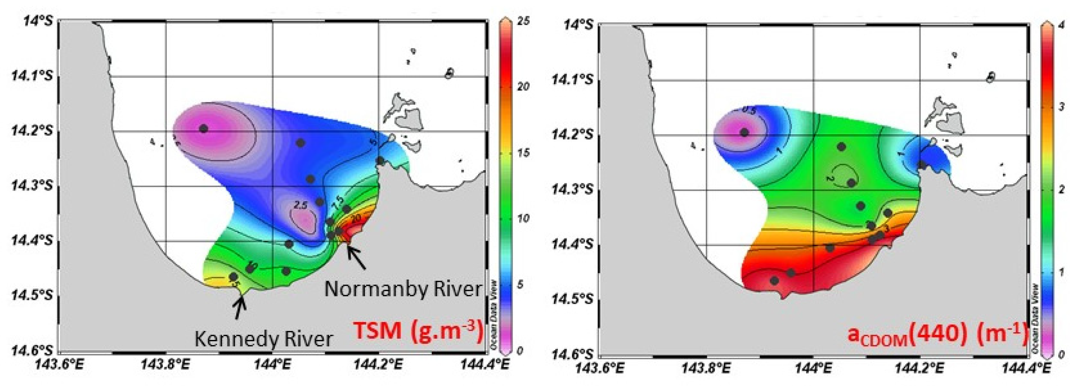
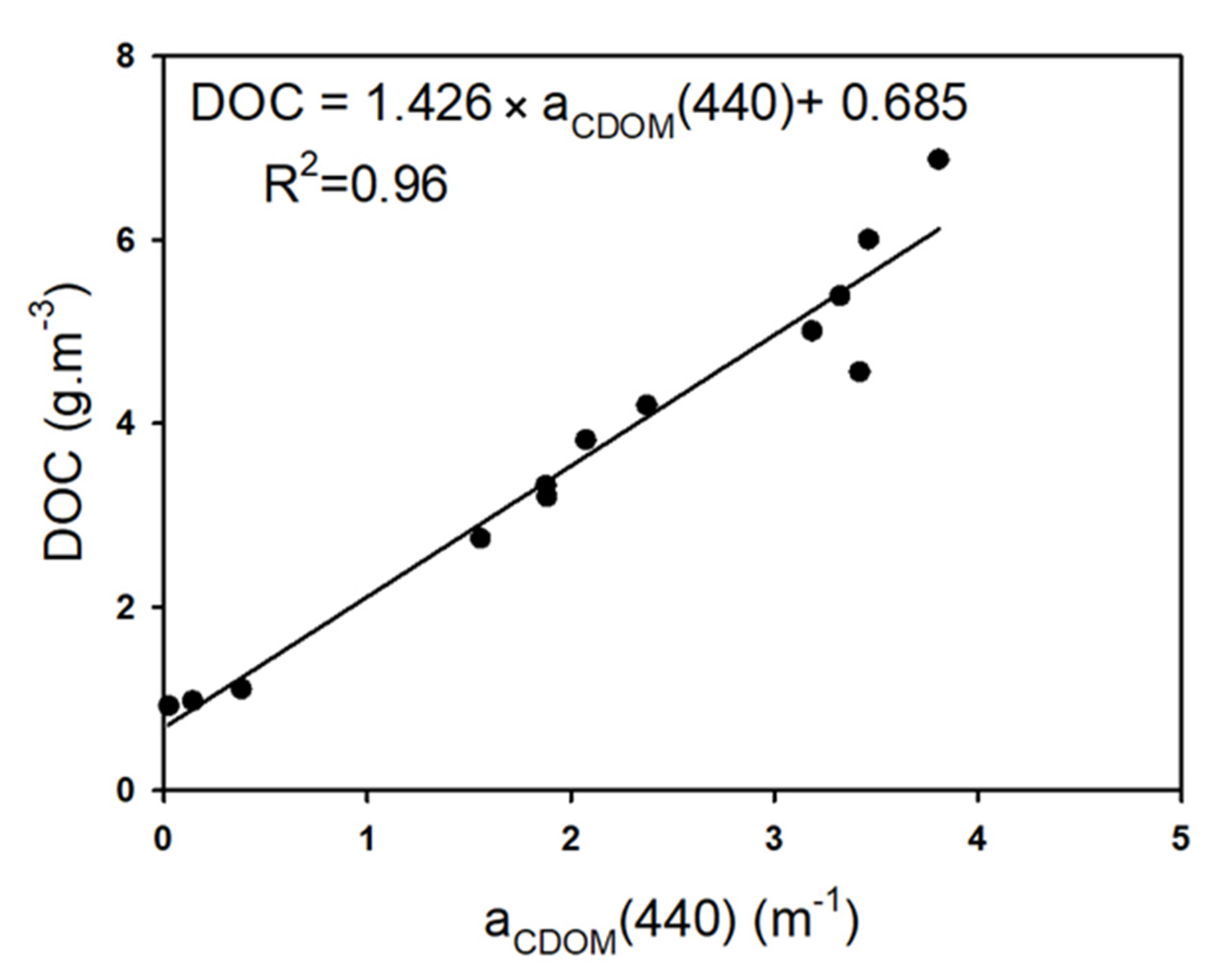
3.3.1. Suspended Solids and Dissolved Organic Matter

PCB was characterized by a strong spatial and temporal biogeochemical variability (Figure 6 and Table 1). Waters closest to the Normanby mouth were highly turbid with a surface Total Suspended Matter concentration (TSM) reaching 23.1 g m⁻³ (st. 1088). TSM dropped by a factor 4 at nearby stations (5.9 and 6.8 g m⁻³ at st. 1089 and 1087 respectively). Near the Kennedy mouth, TSM was also high on 31 January (14.8 g m⁻³ at st. 1093), but much higher on 30 January (as highlighted by the MODIS RGB imagery before we started sampling this region, Figure 3). Interestingly, the repeat station showed a factor 6 drop in TSM over less than 2 days: (from 4.67 to 0.84 g m⁻³). Floodwaters were largely dominated by inorganic particles near the Kennedy mouth (87 and 88% of TSM at st. 1093 and 1092, respectively), and to a lesser extent near the Normanby mouth (82 and 69% at st. 1088 and 1089, respectively). The inorganic contribution dropped significantly outside of the flood plumes (58% in the north of PCB, st. 1095, and 63% near the outer reef, st. 1082). The repeat station showed a nearly 10% drop in the inorganic fraction within 42 h.

The strong biogeochemical variability was reflected in the variability of key in situ bio-optical properties, such as the particle backscattering efficiency at 550 nm (bb_p/b_p(550)) and the TSM-specific scattering coefficient (b*(550)) (Table 1). Both bb_p/b_p(550) and b*(550) are key parameters required to improve satellite ocean color algorithms. bb_p/b_p is an estimate of the fraction of light scattered backwards by particles and also a function of the nature of the particles. bb_p/b_p(550) was high in the floodwaters, with values reaching 4.7% near the Normanby mouth (st. 1088, also with the highest TSM) and 3.3% near the Kennedy mouth (st. 1092). Away from the flood plumes, bb_p/b_p(550) dropped down to 0.5% (st. 1095). In turn, b*(550) increased fivefold from the Normanby mouth to the north of the bay (from 0.23 to 1.05 m² g⁻¹ at st. 1088 and 1095, respectively).

The Dissolved Organic Carbon concentration (DOC) was high near the Kennedy and Normanby mouths (6.88 and 5.39 g m⁻³ at st. 1093 and 1088, respectively) (Table 1). By contrast, in the north of the bay and near the outer-shelf reef, DOC dropped by around a factor 6 to 7 (0.98 and 0.92 g m⁻³ at st. 1095 and 1082, respectively). The absorption coefficient of CDOM a_CDOM, the colored fraction of the dissolved organic matter (so-called ‘gelbstoff’ or yellow substances, [50], dropped by a factor 27 from the Kennedy mouth to the north of the bay (from 3.81 to 0.14 m⁻¹ at 440 nm, at st. 1093 and 1095, respectively). In floodwaters, a_CDOM(440) is a good proxy for DOC. The linear relationship between a_CDOM(440) and DOC is characterized by an R² of 0.96 (p < 0.0001), and the intercept on the Y axis of 0.685 g m⁻³ is representative of the noncolored fraction of DOC (Figure 7). The corresponding a_CDOM*(440) (a_CDOM(440) normalized by DOC) ranged from a maximum of 0.75 and 0.58 m² g⁻¹ near the Normanby and Kennedy mouth (st. 1089 and 1092, respectively) to a minimum of 0.15 and 0.03 m² g⁻¹ in the north of the bay and close to the outer-shelf reef (st. 1095 and 1082, respectively). The repeat station (st. 1084 and 1096) showed a significant drop in a_CDOM*(440) over 42 h (from 0.54 to 0.34 m² g⁻¹, respectively). The CDOM slope ratios (S_275–295/S_350–400) were higher away from the riverine inflows, with less than 1.0 near the rivers and up to ~3.0 in the north of the bay.

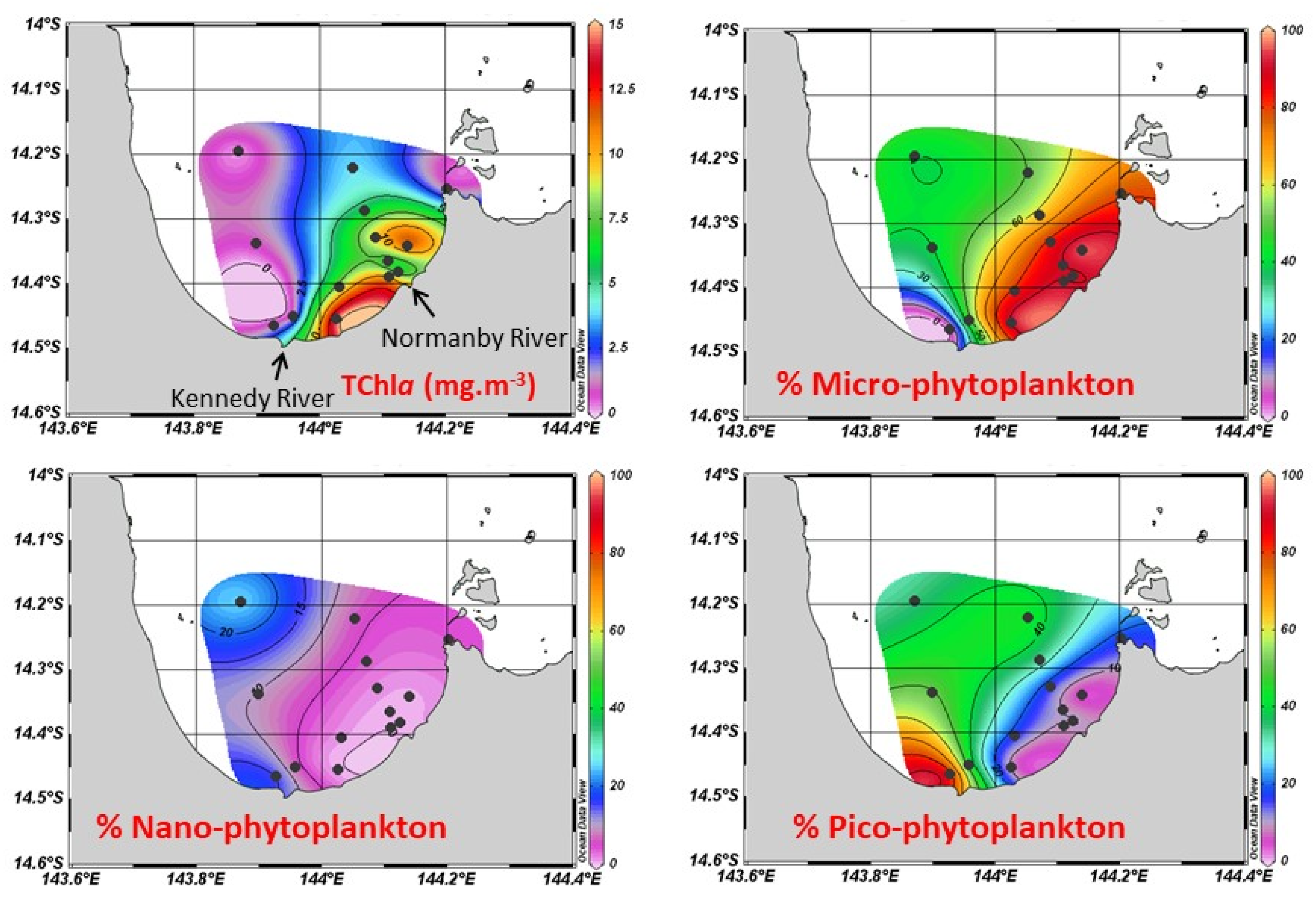
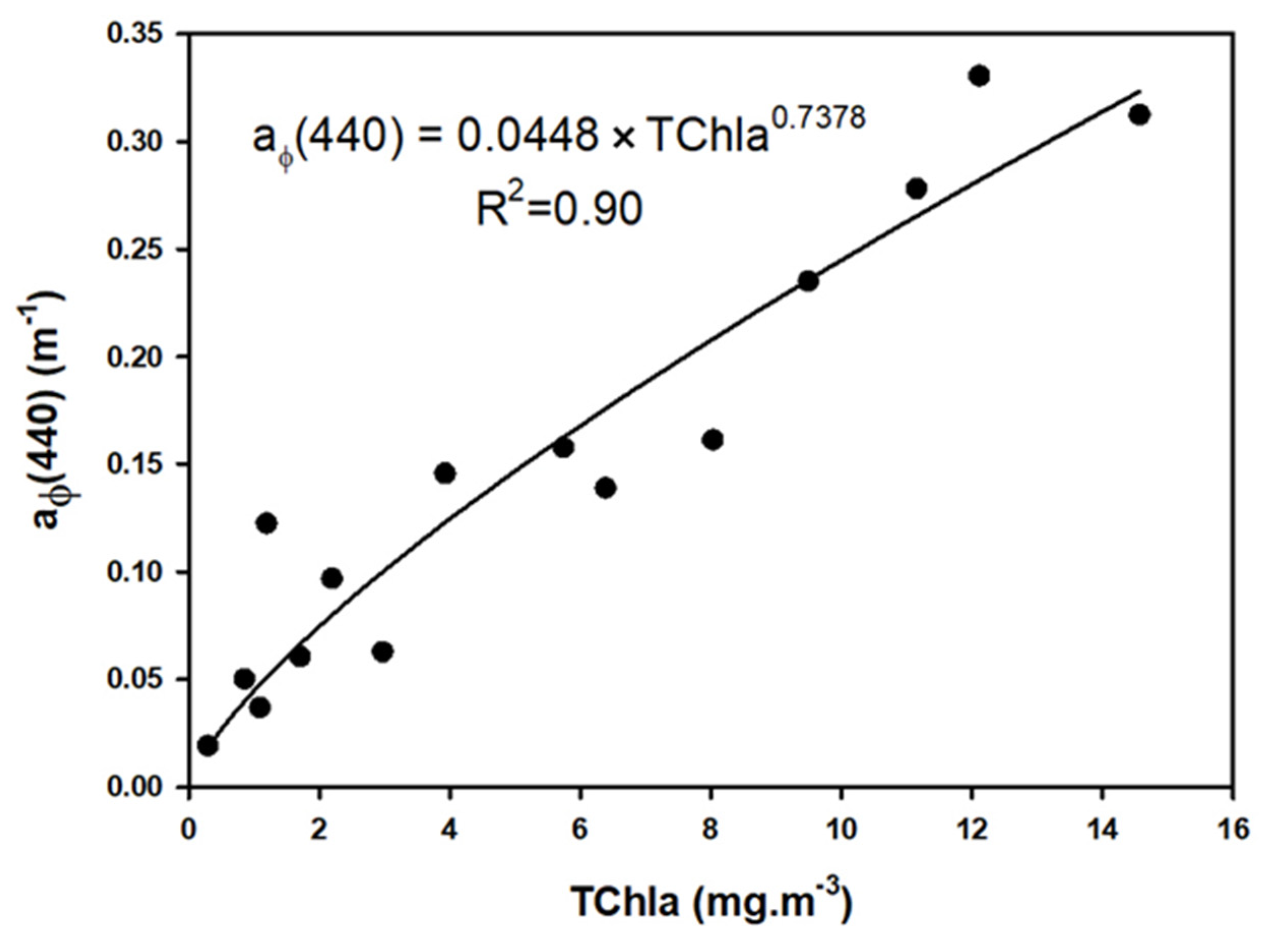
3.3.2. Phytoplankton Biomass and Composition

The most productive waters were located near the mouths of the Bizant and Normanby rivers, with surface TChla concentrations of 14.6 to 11.1 mg m⁻³ at st. 1091 (Bizant) and st. 1089 (Normanby), respectively (Figure 8 and Table 1). This is in contrast with the low values near the Kennedy mouth (0.9 to 1.2 mg m⁻³) and in the clear waters in the north of the bay (0.2 mg m⁻³ st. 1095). Interestingly, the outer-shelf reef waters were productive (~3.0 mg m⁻³ at st. 1082). The repeat station showed a factor 20 drop in TChla (from 5.74 to 0.29 mg m⁻³ at st. 1084 and 1096, respectively).

The phytoplankton composition derived from pigment composition and size indices highlights the predominance of microphytoplankton in the eastern section of the bay under the influence of the Normanby river discharge (91 and 95% at st. 1089 and 1086, respectively) (Figure 8). By contrast, picophytoplankton was dominant in the western section of the bay, with maximum contribution west of the Kennedy mouth (84.6% at st. 1093). Nanophytoplankton accounted for a smaller fraction of the phytoplankton assemblage, with up to 25% in the north of the bay (st. 1095). Microphytoplankton was mainly composed of diatoms (fucoxanthin was the dominant diagnostic pigment). The repeat station (st. 1084 and 1096) showed a strong shift in the phytoplankton composition: the contribution of microphytoplankton decreased from 62.8 to 40.3% within 42 h.

The phytoplankton absorption coefficient at 440 nm (a_ϕ(440), the chlorophyll absorption maximum in the blue) strongly varied across the bay. The Chla-specific absorption coefficient at 440 nm (a_ϕ(440) normalized by TChla) is a key specific inherent optical property for accurate chlorophyll a estimations using ocean color remote sensing algorithms. Over the large range of conditions encountered, a_ϕ(440) and TChla remained highly correlated through a power relationship (a_ϕ(440) = 0.0448*TChla^0.738, R² = 0.90, p < 0.0001; Figure 9).

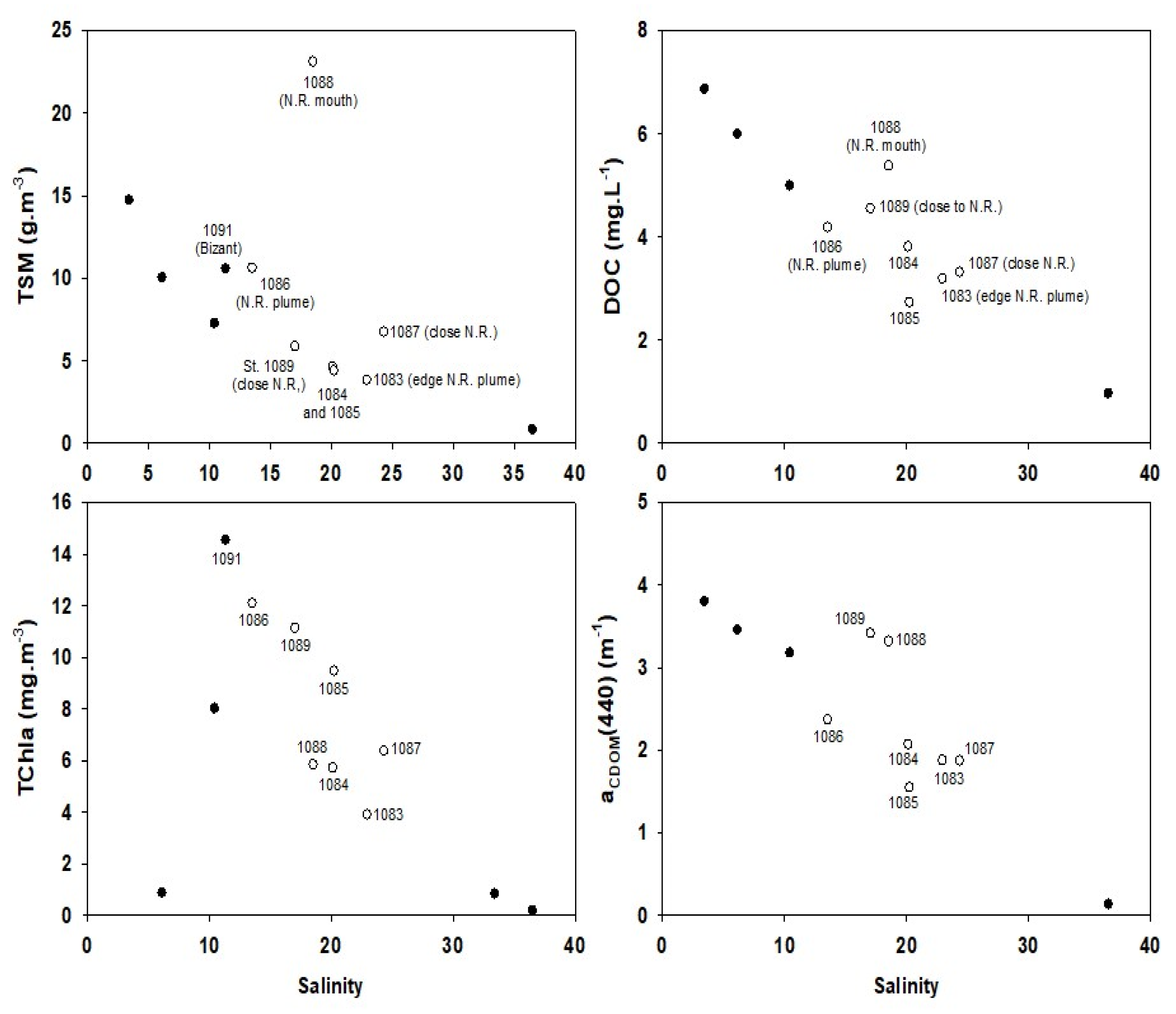
3.4. Biogeochemical Quantities versus Salinity

The relationships between DOC and the CDOM absorption coefficient at 440 nm with salinity (Figure 10) showed an overall decrease with increasing salinity. However, significant departure from the inverse linear trend occurred in the salinity range 15–20, corresponding to the Normanby river outflows (st. 1088 and 1089). In this salinity range, DOC and the CDOM absorption coefficient at 440 nm were significantly higher than expected for a simple mixing model between marine and freshwater end-members. TSM and TChla were, as expected, subject to a nonconservative behavior.

3.5. Absorption Budget

The absorption budget (relative contribution of phytoplankton, nonalgal particles and CDOM to the absorption coefficient) provides information on the main contributors to the absorption coefficient in the surface layer (Figure 11, Table 1). The absorption budget highlights the strong nonalgal particles contribution in the western section of the bay, with around 50% of the total absorption coefficient at 440 nm (st. 1093). By contrast, CDOM dominated the absorption coefficient in the eastern section of the bay (more than 80% at st. 1087 and 1089, and 63% at st. 1088 closest to the Normanby mouth). Phytoplankton absorption was lower than 10% at most stations across PCB and decreased inshore, with minimum values near the Kennedy mouth (4% of the total absorption at st. 1093). Interestingly, at the outer-shelf reef station, the phytoplankton contribution reached ~60 % (st. 1082). The repeat station (st. 1084 and 1096) highlights a significant drop (10%) in the contribution of nonalgal particles in less than 2 days, counterbalanced by a similar increase in the CDOM contribution (Table 1).

4. Discussion

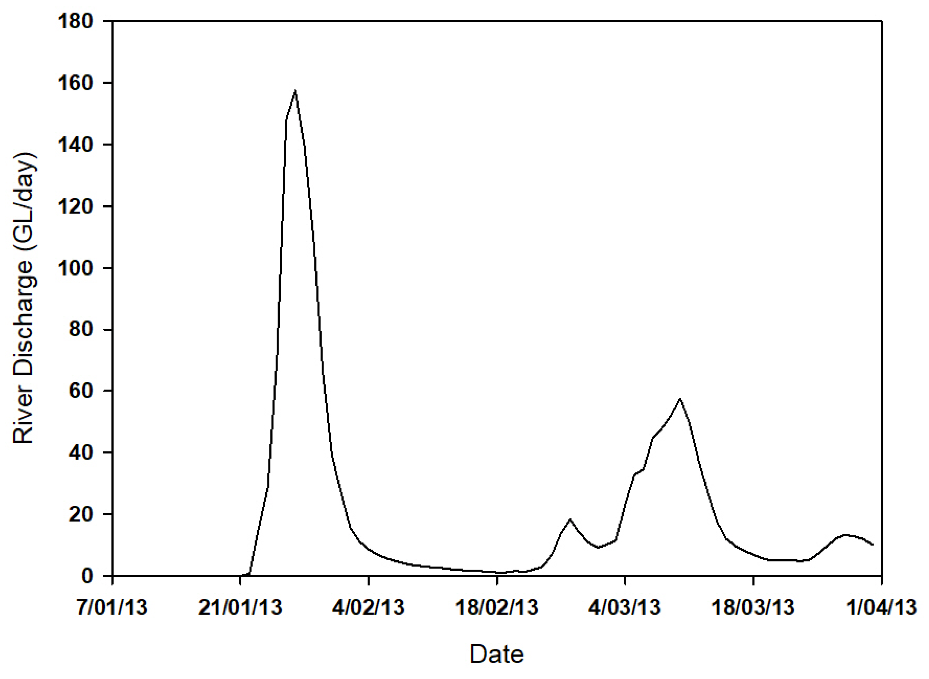
4.1. From Catchment to Coast: Drivers of Riverine Inputs and Impact on Optical Properties

The combined use of ocean color remote sensing and ship-based in situ data highlights the drastic but short-lived changes in PCB following the passage of tropical cyclone Oswald. Despite its widespread damage of human property and infrastructure, its impact on coastal waters appears to be within average values. The strong northwesterly winds (average speed of 13 knots), combined with the local density-driven circulation, lead to an overall North-East extent of the floodwaters, covering a surface of 1400 km². This extent can be compared with long-term average remote sensing observations acquired between 2003 and 2010 (MODIS Terra and Aqua, [30]. Remotely sensed CDOM, used as a surrogate for salinity to estimate the extent of fresh water plumes [28], showed that floodwaters affected outer-shelf reefs in the north of PCB only once during this period. The in situ riverine discharge into the bay, and associated sediment and nutrients loads, were comparable with previous values measured in 2012 and 2014 for the Normanby river [32]. The total river discharge was intermediate between 2012 and 2014 values (860 GL in 2013 against 555 and 1082 GL in 2012 and 2014, respectively) and below long-term average values [32]. The peak TSM (23.1 g m⁻³) was comparable with the corresponding 2012–2014 mean values (21 g m⁻³, [32]. Previous studies were mostly focused on the Normanby river; this work provides key novel insights into the respective roles of the main rivers flowing into PCB: the Kennedy, Bizant and Normanby rivers.

On 30 January, the spatial distributions of biogeochemical and optical properties appeared strongly contrasted due to high loads of diverse riverine inputs, differences in the temporal dynamics for each flood plume, and the mixing between floodwaters from different rivers (Figure 4 and Figure 5). In the western section of the bay, the Kennedy river sediment-laden flood plume was clearly delineated, thus pointing to recent inputs. One day later, on 31 January (day of the inshore field sampling), TSM dropped drastically, CDOM extended further offshore and its relative contribution increased (Figure 5 and Table 1). The low salinity and high DIN confirm recent outflows, resulting in a high inorganic contribution to suspended solids (more than 80%, Table 1). In the eastern section of the bay, the CDOM/phytoplankton predominance points to a more ‘mature’ flood plume on 31 January. A large and clearly delineated sediment-laden flood plume was likely coincident with the peak outflows from the Normanby river on 29 January, but sediments would have mostly dissipated by 30 January when cloud-free remote sensing imagery became available, and even further by 31 January when we started the inshore field sampling. Cloud cover is a major limitation of satellite applications after flood events.

The drastic changes in the nature of the particulate and dissolved organic materials resulted in significant changes in the IOPs (magnitude and spectral slopes) and SIOPs (Table 1). Here, we only discuss the variability in IOPs and SIOPs, which are essential for accurate retrievals of biogeochemical quantities using ocean color remote sensing algorithms. The actual algorithms development was examined elsewhere [30]. The inshore predominance of mineral particles translates into low scattering per unit of suspended matter mass concentration (b*(550), Table 1). The inshore values of the backscattering efficiency (bb_p/b_p(550)) and the TSM-specific scattering coefficient (b*(550)) values are in the range expected for mineral dominated particles, in agreement with their predominantly inorganic nature [51] and references therein). Near the mouth of the Kennedy river, the nonalgal particles (including mineral particles) contribution to the absorption coefficient is particularly high. In the north of the bay, the predominance of phytoplankton and organic particles with a lower apparent density lead to a low bb_p/b_p(550) and high b*(550).

The repeat station provides a snapshot view of the rapid and nonlinear changes in both the amount and nature of particulate and dissolved organic materials over time (Table 1). From 30 January to 1 February, the 15 units increase in salinity was associated with a large drop in particle, phytoplankton and dissolved materials concentrations (nearly a factor 6 decrease in TSM and CDOM and a factor 20 drop in TChla), and a decrease in their terrestrial signature (e.g., drop in the TSM inorganic fraction and a_CDOM*(440), and increase in the spectral slope ratios). Within 10 days (09 February), remotely sensed suspended solids and CDOM were similar to baseline conditions preflood. This is based on observations made on 14 January (Figure 4), as TCO lead to a ‘first flush’ event (no significant rains were recorded previously during this wet season). Preflood conditions are often missing due to the difficulty in planning a field survey prior to episodic events; remote sensing imagery is an alternative approach during cloud-free conditions.

Interestingly, the wide range of concentrations sampled within PCB encompass those encountered in the mid- to northern GBR inshore waters postfloods during the same wet season (e.g., in the Daintree, Annan and Burdekin rivers, [25]). Long-term records of suspended solids concentration from the Burdekin and Fitzroy rivers, the two largest GBR dry-tropics catchments, highlight the comparatively much lower suspended solids loads into PCB. By contrast, CDOM and DOC were generally higher than for urbanized catchments [51,52,53]. Intensive catchment land use through agriculture and urbanization is responsible for increased suspended solids inputs into the coastal zone (e.g., Moreton Bay [51]), Galveston Bay [5], Chesapeake Bay [54] and the Yangtze River, [55]. The Normanby and Kennedy catchments are relatively pristine, resulting in a lower potential for sediments mobilization during rain events. However, ‘first flush’ events are associated with more sediment mobilization due to the low vegetation cover during the previous dry season, and the type of material mobilized differs [32,56,57,58].

Concurrent characterizations of the optical and biogeochemical properties of coastal waters following a major episodic flood event are scarce and often limited in time. In 2011, we used a similar bio-optical approach to examine the impact of catastrophic and widespread floods in Moreton Bay, adjacent to the city of Brisbane (East coast of Australia), over a one year period. Interestingly, the maximum values in PCB were in the same range as those measured inshore one week after the ‘Brisbane floods’: for the suspended solids concentration, near the mouth of the highly urbanized Brisbane river; and for CDOM, in Deception Bay (in the north-west of Moreton Bay) where the upper catchment is covered by large areas of natural vegetation [51]. The latter was likely responsible for the higher CDOM contribution, similarly to observations made in PCB. However, Moreton Bay and PCB differ in terms of vegetation type/cover and agricultural land use [59]. Previous studies might be biased towards lower IOPs due to field sampling limitations of these highly episodic events. Comparisons between flood events are compounded by catchment characteristics and land use, antecedent rain events and river discharge, wind stress and tidal mixing, local density-driven circulation, as well as sampling designs.

4.2. Transformation Processes and Critical Time Scales

Particles and CDOM dynamics are driven by complex interactions between physical, biogeochemical and biological processes (primary production, microbial degradation and zooplankton grazing) and photodegradation [60,61]. Sediment resuspension is driven by tidal asymmetry, wind stress and local density-driven circulation. Tides can change the size and nature of particles via resuspension, aggregation–disaggregation and flocculation [62], and contribute an important source of CDOM in shallow waters (e.g., [33,63]). The strong northwesterly winds (average speed of 13 knots) contributed to large-scale sediment resuspension from the shallow bottom. Tides also skew the spatial observations, and are often not taken into account during the sampling design and the interpretation of remote sensing imagery [64]. Satellite overpasses are at fixed times of the day, while high tide/low tide times shift on a daily basis. Coupling between biogeochemical modelling and ocean color remote sensing algorithms has been used as one solution to overcome these limitations (e.g., [12,65]). The respective roles of tidal-driven and wind-driven resuspension are unknown and require further study, either through specifically designed in situ process studies and/or modelling.

During the 2016–2017 dry season, [33] showed that the surface to bottom increase in TSM could reach up to a factor 10 in the mixing zone during spring tides (tidal current velocity of up to 2.1 m s⁻¹). Due to differences in channel bathymetry and habitats, maximum tidal current velocities at the mouth of the Kennedy river can be double those at the mouth of the Normanby river, and result in an average TSM value four times higher [33]. During the wet season, bottom sediments were dominated by silt to fine sand near the estuary mouths [33], which can be easily remobilized in the water column. During our study, the tidal currents were relatively weak (0.3–0.6 m s⁻¹). The vertical distribution data points to an increase in particulate attenuation from the surface to bottom by only up to a factor 2, and a mainly freshwater source of CDOM (data not shown).

Differences in the sources of materials and mixing between floodwaters from the different rivers increase the complexity of near-shore coastal processes. The main estuaries in the south of the bay are well connected during the wet season, with mixing between riverine end-members in the coastal floodplains. In addition, the mainly north-eastward direction of the flood plumes likely lead to further mixing in the eastern section of the bay. Dissolved organic matter parameters mainly followed a conservative mixing behavior in the western section under the influence of the Kennedy river outflows (Figure 10). By contrast, the strong deviations from a classical mixing trend in the eastern section of the bay, at several stations in the salinity range 15–20, highlight different sources of DOC/CDOM. At St. 1088 and 1089 (near the Normanby river mouth and slightly to the left of the main flood plume, respectively), DOC and CDOM values for a given salinity were markedly above the general trend. St. 1089 was characterized by the highest terrestrial signature, as depicted by a_CDOM*(440), followed by 1088 and 1087 (Table 1). St. 1088 was also the station with the highest TSM, and likely represents the ‘end-member’ of the terrestrial inputs from the Normanby river.

The sources of DOC and CDOM can be allochthonous (terrestrial inputs) or autochthonous (produced in situ) [66]. Sources of dissolved organic matter from the salt flats also contribute to a large fraction of the inshore CDOM. At St. 1089, where TChla is high, the production of dissolved organic matter by phytoplankton also needs to be taken into account [67]. Terrestrial inputs and phytoplankton-derived dissolved organic matter will then undergo rapid transformation processes through microbial degradation [68] and/or photodegradation. The UV spectral data and a_CDOM*(440) offer insights into the nature and transformation processes affecting CDOM. There is a strong dichotomy between the near-shore waters, which are mostly CDOM of higher molecular weight indicative of fresh terrestrial organic matter, and offshore waters dominated by lower molecular weight dissolved organic material with spectral slope ratios of around 3 (north of PCB and outer-shelf reef station, Table 1). The later are indicative of strong photodegradation and uptake by the microbial compartment. The CDOM absorption in the UV is approximately 10% of that of the riverine affected waters. Due to the considerable photodegradation, the source of CDOM cannot be inferred from the UV spectral characteristics. Empirical relationships between the CDOM absorption coefficient and DOC concentration established for remote sensing applications are often region and season-specific [53,69,70].

The residence time (the amount of time a water parcel stays in a given area) is a critical factor regulating the cycling of terrestrial inputs in coastal ecosystems and the resulting phytoplankton response [4,71,72]. It is a function of the discharge volume relative to the volume of the bay, the density-driven circulation, the tidal regime and wind conditions, and can range from days to weeks [33]. [73] showed that water column nutrient recycling was an order of magnitude higher than riverine input. The apparent rapid return to preflood conditions can be explained by the rapid time scales of the transformation processes in tropical and subtropical systems [51,74] and references therein). Lack of proper quantification of the particulate and dissolved materials and carbon fluxes from the catchment to the reef will lead to a large underestimation in regional and global biogeochemical budgets. This is particularly critical in the context of increasing changes in catchment land use, the subsequent degradation of water quality draining these catchments, and the increase in sediment and particle loads flowing into the coastal zone.

The transformation processes of the terrestrial inputs in the coastal zone occur within hours to days, and result in drastic changes in the IOPs and SIOPs. Quantifying SIOPs variability across the short spatial and temporal scales during flood conditions (across PCB, at a given point along the tidal cycle, and from the peak riverine discharge to the last of the riverine outflows) is a major challenge for accurate estimations of ocean color products and for underwater light climate models. Similar observations in subtropical and tropical systems (e.g., [51,75,76]) highlight the critical need for a better knowledge of SIOPs (TSM, Chla or DOC-specific optical coefficients) across different coastal ecosystems and in a given region across a wide range of hydrodynamic conditions (i.e., regionally tuned and ‘event-tuned’ ocean color algorithms).

4.3. Phytoplankton Response

The dynamics of phytoplankton blooms are driven by complex interactions between nutrient inputs, light availability (magnitude and spectral quality), hydrodynamic processes, organic and inorganic pollutants, and loss terms (senescence and zooplankton grazing) [4,5,75,77,78,79]. Previous studies have highlighted contrasting and event-specific responses to floods, from large phytoplankton blooms [75] and references therein) to a reduction of phytoplankton biomass [80]. During the present study, flood-derived bioavailable nutrients were favorable to primary production (e.g., DIN of up to 5.8 μM near the Kennedy mouth), while high loads of particles and CDOM strongly reduced light availability. Phytoplankton growth was optimal at midsalinities where TSM was lower than 10 g m⁻³ and DIN concentration was still high, in agreement with previous observations in tropical and subtropical regions (e.g., Brisbane, Amazon, Changjiang, and Mississippi rivers) [51,75] and references therein). The maximum TChla (14.6 mg m⁻³) was in the intermediate zone between the Kennedy and Normanby flood plumes, where water clarity increased due to a sharp drop in TSM despite a high CDOM content.

The highest TChla was similar to values encountered one week after the 2011 extreme Brisbane floods in Deception Bay (north-west of Moreton Bay, 12.0 mg m⁻³, [51], where the suspended solids content was lower but CDOM was still relatively high. CDOM is seldom characterized during flood conditions but remains a key driver of the underwater light availability for primary production. A better description of the light exposure and nutrient availability in floodwaters in the hours/days prior to a phytoplankton bloom is essential to understand the phytoplankton community response. The in situ variability in the phytoplankton response across the bay (eastern and western sections) on 31 January reflects the different ‘stages’ of rapidly changing flood plumes and the resulting phytoplankton response: from recent outflows from the Kennedy river, where phytoplankton didn’t bloom yet despite high DIN values (due to the high TSM), to a more ‘mature’ flood plume in the ‘mixing’ zone with the Normanby river outflows, where phytoplankton growth conditions were optimum (uptake of DIN leading to a higher TChla, Table 1).

The high TChla was within the range of other coastal systems following high riverine inflows (e.g., [4,51,75,76,81,82]), but much higher than previously measured in the same region [23,32]. The spatial coverage and timing of our in situ sampling likely provided a more complete picture of the phytoplankton dynamics postflood than previous studies, despite missing the peak riverine discharge from the Normanby river on 29 January. Comparisons between the phytoplankton community response after different flood events are difficult due to sampling different stages of rapidly changing phytoplankton blooms, differing hydrodynamic conditions and using different methodological setups. The burst of phytoplankton growth is usually short-lived in subtropical and tropical systems [75], due to nutrient consumption, dilution/dispersion processes, and loss terms (senescence and zooplankton grazing).

In the eastern section of the bay, diatoms were predominant with more than 90% of the phytoplankton population. Skeletonema spp. was identified as the dominant species [32]. Diatoms are usually the first species to bloom in response to large nutrients inputs (PCB [32,33], and elsewhere [75,79,83,84]. The presence of diatoms confirms the more ‘mature’ characteristics of floodwaters in this region, when phytoplankton already had the time to bloom. This is in contrast with floodwaters from the Kennedy river, where picophytoplankton and the signature of nonalgal particles were predominant (as depicted by the absorption budget, the TSM-specific scattering coefficient and the TSM inorganic fraction). Unfortunately, information on the local phytoplankton communities prior to the January 2013 floods is a major missing point. This is essential for better predictions of the phytoplankton response postfloods. Previous studies in subtropical systems pointed to the picophytoplankton cyanobacteria as the dominant group during periods of low river discharge [75,84,85].

Changes in the phytoplankton community composition and photoadaptation status lead to the observed variability in the relationship between the absorption coefficient at 440 nm and TChla, a key factor to improve ocean color remote sensing algorithms for phytoplankton studies in coastal waters. The relationship established across the whole of PCB is significantly different from parameterizations in other environments in Australia: across a large range of inshore and reef waters of the GBR lagoon (a_ϕ(440) = 0.0500*TChla^0.647, [86], and following the extreme 2011 Brisbane floods (a_ϕ(440) = 0.0663*TChla^0.633, [51]. This relationship is mainly driven by cellular pigment composition and the pigment packaging effect (the package effect is an inverse function of cell size and intracellular pigment concentration; [87]. As a result, the lowest a_ϕ∗(440) values are associated with the presence of diatoms (higher package effect and thus decrease in a_ϕ∗(440)).

Alternative ocean color remote sensing-based methods were used in the past to access quantitative information on phytoplankton composition immediately prior to and after major flood events. These approaches mainly rely on the decomposition of the phytoplankton absorption coefficient into respective pigments concentrations (e.g., using a non-negative least square algorithm, [4,6,75]), or by deriving phytoplankton functional types or PFT, [88] or the estimation of a phytoplankton size index [89]. These alternative approaches are not the aim of the present paper but mentioned here as they open up a whole range of possibilities for coastal applications (e.g., daily description of the dominant phytoplankton groups over the course of a flood event). However, in situ data collection is still required to test and regionally tune these algorithms, and provide detailed information on the phytoplankton composition.

5. Conclusions

The widespread flooding associated with the passage of tropical cyclone Oswald over the northern GBR resulted in large and highly episodic riverine inputs into Princess Charlotte Bay (PCB). Floodwaters from the Kennedy, Bizant and Normanby rivers lead to contrasted physical, biogeochemical and bio-optical properties between inshore and offshore waters, and between the western and eastern sections of PCB. Differences in the riverine loads and nature, the timing of the peak riverine outflows (e.g., Kennedy vs Normanby), and the phytoplankton response and transformation processes within PCB contributed to contrasted observations. Despite being limited in time and space (snapshot view), the fortuitous timing of our field sampling provides powerful insights into the respective roles of the different rivers on the biogeochemical processes occurring in the coastal zone.

There is a strong need for long-term studies on the impact of extreme events on inputs to the coastal zone and the resilience of the adjacent coastal ecosystems (from seagrass meadows to coral reefs and fisheries). The implementation of long-term monitoring programs is key to constrain the full range of variability in IOPs and SIOPs in complex and dynamic systems such as the GBR. While logistically difficult on an ad-hoc basis using conventional field sampling strategies, partnerships between local industry, community groups and research teams could bring synergies for a better in situ characterization of these highly episodic events, particularly in remote areas. The differences in the sources/nature of materials coming from the different catchments and the transformation processes within the respective rivers before reaching the coastal zone need to be accounted for (e.g., stable isotopes studies).

Once ‘regionally’ and ‘event’ tuned ocean color algorithms are developed, remote sensing approaches will provide powerful tools to quantify and characterize flood inputs into the coastal zone. Comprehensive biogeochemical/bio-optical and in situ/remote sensing studies, from catchments to coast, across a wide range of conditions (e.g., during a complete wet season with successive rain events and across a large range of tidal conditions) and ecosystems is key in improving regional and global budgets. Such approaches can ultimately be incorporated into catchment management strategies and mitigation approaches to reduce sediment and nutrient loads into the GBR and other high value coastal ecosystems around the world.

References

1. Bauer, J.E.; Cai, W.J.; Raymond, P.A.; Bianchi, T.S.; Hopkinson, C.S.; Regnier, P.A. The changing carbon cycle of the coastal ocean. Nature 2013, 504, 61–70. [Google Scholar] [CrossRef] [PubMed]
2. Van Vliet, M.T.; Franssen, W.H.; Yearsley, J.R.; Ludwig, F.; Haddeland, I.; Lettenmaier, D.P.; Kabat, P. Global river discharge and water temperature under climate change. Glob. Environ. Chang. 2013, 23, 450–464. [Google Scholar] [CrossRef]
3. Kundzewicz, Z.W.; Szwed, M.; Pinskwar, I. Climate Variability and Floods—A Global Review. Water 2019, 11, 1399. [Google Scholar] [CrossRef] [Green Version]
4. Liu, B.Q.; D’Sa, E.J.; Joshi, I.D. Floodwater impact on Galveston Bay phytoplankton taxonomy, pigment composition and photo-physiological state following Hurricane Harvey from field and ocean color (Sentinel-3A OLCI) observations. Biogeosciences 2019, 16, 1975–2001. [Google Scholar] [CrossRef] [Green Version]
5. Steichen, J.L.; Labonte, J.M.; Windham, R.; Hala, D.; Kaiser, K.; Setta, S.; Faulkner, P.C.; Bacosa, H.; Yan, G.; Kamalanathan, M.; et al. Microbial, Physical, and Chemical Changes in Galveston Bay Following an Extreme Flooding Event, Hurricane Harvey. Front. Mar. Sci. 2020, 7, 186. [Google Scholar] [CrossRef]
6. D’Sa, E.J.; Joshi, I.D.; Liu, B.Q.; Ko, D.S.; Osburn, C.L.; Bianchi, T.S. Biogeochemical Response of Apalachicola Bay and the Shelf Waters to Hurricane Michael Using Ocean Color Semi-Analytic/Inversion and Hydrodynamic Models. Front. Mar. Sci. 2019, 6, 523. [Google Scholar] [CrossRef] [Green Version]
7. D’Sa, E.J.; Joshi, I.; Liu, B.Q. Galveston Bay and Coastal Ocean Optical-Geochemical Response to Hurricane Harvey from VIIRS Ocean Color. Geophys. Res. Lett. 2018, 45, 10579–10589. [Google Scholar] [CrossRef] [Green Version]
8. Cherukuru, N.; Brando, V.E.; Schroeder, T.; Clementson, L.A.; Dekker, A.G. Influence of river discharge and ocean currents on coastal optical properties. Cont. Shelf Res. 2014, 84, 188–203. [Google Scholar] [CrossRef]
9. Eccles, R.; Zhang, H.; Hamilton, D. A review of the effects of climate change on riverine flooding in subtropical and tropical regions. J. Water Clim. Chang. 2019, 10, 687–707. [Google Scholar] [CrossRef] [Green Version]
10. Paerl, H.W.; Crosswell, J.R.; Van Dam, B.; Hall, N.S.; Rossignol, K.L.; Osburn, C.L.; Hounshell, A.G.; Sloup, R.S.; Harding, L.W. Two decades of tropical cyclone impacts on North Carolina’s estuarine carbon, nutrient and phytoplankton dynamics: Implications for biogeochemical cycling and water quality in a stormier world. Biogeochemistry 2018, 141, 307–332. [Google Scholar] [CrossRef]
11. Baird, M.E.; Mongin, M.; Rizwi, F.; Bay, L.K.; Cantin, N.E.; Morris, L.A.; Skerratt, J. The effect of natural and anthropogenic nutrient and sediment loads on coral oxidative stress on runoff-exposed reefs. Mar. Pollut. Bull. 2021, 168, 112409. [Google Scholar] [CrossRef] [PubMed]
12. Baird, M.E.; Mongin, M.; Skerratt, J.; Margvelashvili, N.; Tickell, S.; Steven, A.D.L.; Robillot, C.; Ellis, R.; Waters, D.; Kaniewska, P.; et al. Impact of catchment-derived nutrients and sediments on marine water quality on the Great Barrier Reef: An application of the eReefs marine modelling system. Mar. Pollut. Bull. 2021, 167, 112297. [Google Scholar] [CrossRef] [PubMed]
13. Lewis, S.E.; Bartley, R.; Wilkinson, S.N.; Bainbridge, Z.T.; Henderson, A.E.; James, C.S.; Irvine, S.A.; Brodie, J.E. Land use change in the river basins of the Great Barrier Reef, 1860 to 2019: A foundation for understanding environmental history across the catchment to reef continuum. Mar. Pollut. Bull. 2021, 166, 112193. [Google Scholar] [CrossRef] [PubMed]
14. Wolff, N.H.; Mumby, P.J.; Devlin, M.; Anthony, K.R.N. Vulnerability of the Great Barrier Reef to climate change and local pressures. Glob. Chang. Biol. 2018, 24, 1978–1991. [Google Scholar] [CrossRef] [Green Version]
15. Devlin, M.J.; Petus, C.; da Silva, E.; Tracey, D.; Wolff, N.H.; Waterhouse, J.; Brodie, J. Water Quality and River Plume Monitoring in the Great Barrier Reef: An Overview of Methods Based on Ocean Colour Satellite Data. Remote Sens. 2015, 7, 12909–12941. [Google Scholar] [CrossRef] [Green Version]
16. Brodie, J.E.; Kroon, F.J.; Schaffelke, B.; Wolanski, E.C.; Lewis, S.E.; Devlin, M.J.; Bohnet, I.C.; Bainbridge, Z.T.; Waterhouse, J.; Davis, A.M. Terrestrial pollutant runoff to the Great Barrier Reef: An update of issues, priorities and management responses. Mar. Pollut. Bull. 2012, 65, 81–100. [Google Scholar] [CrossRef]
17. Petus, C.; Waterhouse, J.; Lewis, S.; Vacher, M.; Tracey, D.; Devlin, M. A flood of information: Using Sentinel-3 water colour products to assure continuity in the monitoring of water quality trends in the Great Barrier Reef (Australia). J. Environ. Manag. 2019, 248, 109255. [Google Scholar] [CrossRef]
18. Hughes, T.P.; Barnes, M.L.; Bellwood, D.R.; Cinner, J.E.; Cumming, G.S.; Jackson, J.B.C.; Kleypas, J.; van de Leemput, I.A.; Lough, J.M.; Morrison, T.H.; et al. Coral reefs in the Anthropocene. Nature 2017, 546, 82–90. [Google Scholar] [CrossRef] [PubMed] [Green Version]
19. McCulloch, M.; Fallon, S.; Wyndham, T.; Hendy, E.; Lough, J.; Barnes, D. Coral record of increased sediment flux to the inner Great Barrier Reef since European settlement. Nature 2003, 421, 727–730. [Google Scholar] [CrossRef] [PubMed]
20. Kroon, F.J.; Kuhnert, P.M.; Henderson, B.L.; Wilkinson, S.N.; Kinsey-Henderson, A.; Abbott, B.; Brodie, J.E.; Turner, R.D.R. River loads of suspended solids, nitrogen, phosphorus and herbicides delivered to the Great Barrier Reef lagoon. Mar. Pollut. Bull. 2012, 65, 167–181. [Google Scholar] [CrossRef]
21. Carlson, R.R.; Foo, S.A.; Asner, G.P. Land Use Impacts on Coral Reef Health: A Ridge-to-Reef Perspective. Front. Mar. Sci. 2019, 6, 562. [Google Scholar] [CrossRef]
22. Schaffelke, B.; Carleton, J.; Skuza, M.; Zagorskis, I.; Furnas, M.J. Water quality in the inshore Great Barrier Reef lagoon: Implications for long-term monitoring and management. Mar. Pollut. Bull. 2012, 65, 249–260. [Google Scholar] [CrossRef] [PubMed]
23. Waterhouse, J.; Gruber, R.; Logan, M.; Petus, C.; Howley, C.; Lewis, S.; Tracey, D.; James, C.; Mellors, J.; Tonin, H. Marine Monitoring Program: Annual Report for Inshore Water Quality Monitoring 2019–2020; Great Barrier Reef Marine Park Authority: Townsville, QLD, Australia, 2021. [Google Scholar]
24. Steven, A.D.L.; Baird, M.E.; Brinkman, R.; Car, N.J.; Cox, S.J.; Herzfeld, M.; Hodge, J.; Jones, E.; King, E.; Margvelashvili, N.; et al. eReefs: An operational information system for managing the Great Barrier Reef. J. Oper. Oceanogr. 2019, 12, S12–S28. [Google Scholar] [CrossRef] [Green Version]
25. Cherukuru, N.; Anstee, J.; Oubelkheir, K.; Ford, P.; Clementson, L.; Brando, V.; Schroeder, T.; King, E.; Steven, A. eReefs Wet Season Bio-Optics Field Sampling and Remote Sensing Algorithm Evaluation Report; Commonwealth Scientific and Industrial Research Organisation: Canberra, NSW, Australia, 2015. [Google Scholar]
26. Brando, V.E.; Braga, F.; Zaggia, L.; Giardino, C.; Bresciani, M.; Matta, E.; Bellafiore, D.; Ferrarin, C.; Maicu, F.; Benetazzo, A.; et al. High-resolution satellite turbidity and sea surface temperature observations of river plume interactions during a significant flood event. Ocean Sci. 2015, 11, 909–920. [Google Scholar] [CrossRef] [Green Version]
27. King, E.; Schroeder, T.; Brando, V.; Suber, K. A Pre-Operational System for Satellite Monitoring of Great Barrier Reef Marine Water Quality; CSIRO: Hobart, TAS, Australia, 2014. [Google Scholar] [CrossRef]
28. Schroeder, T.; Devlin, M.J.; Brando, V.E.; Dekker, A.G.; Brodie, J.E.; Clementson, L.A.; McKinna, L. Inter-annual variability of wet season freshwater plume extent into the Great Barrier Reef lagoon based on satellite coastal ocean colour observations. Mar. Pollut. Bull. 2012, 65, 210–223. [Google Scholar] [CrossRef]
29. Schroeder, T.; Lovell, J.; King, E.; Clementson, L.A.; Scott, R. IMOS Ocean Colour Validation Report 2015–2016; CSIRO: Hobart, TAS, Australia, 2016; p. 33. [Google Scholar]
30. Brando, V.; Schroeder, T.; King, E.; Dyce, P. Reef Rescue Marine Monitoring Program: Using Remote Sensing for GBR-Wide Water Quality; Final Report for 2012/13 Activities; Commonwealth Scientific and Industrial Research Organisation: Canberra, NSW, Australia, 2015. [Google Scholar]
31. Deng, D.F.; Ritchie, E.A. Rainfall Mechanisms for One of the Wettest Tropical Cyclones on Record in Australia-Oswald (2013). Mon. Weather Rev. 2020, 148, 2503–2525. [Google Scholar] [CrossRef] [Green Version]
32. Howley, C.; Devlin, M.; Burford, M. Assessment of water quality from the Normanby River catchment to coastal flood plumes on the northern Great Barrier Reef, Australia. Mar. Freshw. Res. 2018, 69, 859–873. [Google Scholar] [CrossRef]
33. Crosswell, J.R.; Carlin, G.; Steven, A. Controls on Carbon, Nutrient, and Sediment Cycling in a Large, Semiarid Estuarine System; Princess Charlotte Bay, Australia. J. Geophys. Res.-Biogeosci. 2020, 125, e2019JG005049. [Google Scholar] [CrossRef]
34. Joo, M.; McNeil, V.H.; Carroll, C.; Waters, D.; Choy, S.C. Sediment and Nutrient Load Estimates for Major Great Barrier Reef Catchments (1987–2009) for Source Catchment Model Validation; Department of Science, Information Technology, Innovation and the Arts: Brisbane, QLD, Australia, 2014. [Google Scholar]
35. McCloskey, G.L.; Baheerathan, R.; Dougall, C.; Ellis, R.; Bennett, F.R.; Waters, D.; Darr, S.; Fentie, B.; Hateley, L.R.; Askildsen, M. Modelled estimates of fine sediment and particulate nutrients delivered from the Great Barrier Reef catchments. Mar. Pollut. Bull. 2021, 165, 112163. [Google Scholar] [CrossRef]
36. Clementson, L.A. The CSIRO Method; NASA Goddard Space Flight Center: Greenbelt, MD, USA, 2013. [Google Scholar]
37. Chase, A.P.; Kramer, S.J.; Haëntjens, N.; Boss, E.S.; Karp-Boss, L.; Edmondson, M.; Graff, J.R. Evaluation of diagnostic pigments to estimate phytoplankton size classes. Limnol. Oceanogr. Methods 2020, 18, 570–584. [Google Scholar] [CrossRef]
38. Vidussi, F.; Claustre, H.; Manca, B.B.; Luchetta, A.; Marty, J.C. Phytoplankton pigment distribution in relation to upper thermocline circulation in the eastern Mediterranean Sea during winter. J. Geophys. Res.-Ocean. 2001, 106, 19939–19956. [Google Scholar] [CrossRef]
39. Uitz, J.; Claustre, H.; Morel, A.; Hooker, S.B. Vertical distribution of phytoplankton communities in open ocean: An assessment based on surface chlorophyll. J. Geophys. Res.-Ocean. 2006, 111, C08005. [Google Scholar] [CrossRef]
40. Peltzer, E.T.; Fry, B.; Doering, P.H.; McKenna, J.H.; Norrman, B.; Zweifel, U.L. A comparison of methods for the measurement of dissolved organic carbon in natural waters. Mar. Chem. 1996, 54, 85–96. [Google Scholar] [CrossRef]
41. Eaton, A.D.; Clesceri, L.S.; Rice, E.W.; Greenberg, A.E.; Franson, M.A.H. Standard Methods for the Examination of Water and Waste Water; American Public Health Association: Washington, DC, USA, 2005; p. 1368. [Google Scholar]
42. Kishino, M.; Takahashi, M.; Okami, N.; Ichimura, S. Estimation of the spectral absorption coefficients of phytoplankton in the sea. Bull. Mar. Sci. 1985, 37, 634–642. [Google Scholar]
43. Mitchell, B. Algorithms for Determining the Absorption Coefficient for Aquatic Particulates Using the Quantitative Filter Technique; SPIE: Washington, DC, USA, 1990; Volume 1302. [Google Scholar]
44. Fichot, C.G.; Benner, R. A novel method to estimate DOC concentrations from CDOM absorption coefficients in coastal waters. Geophys. Res. Lett. 2011, 38, L03610. [Google Scholar] [CrossRef]
45. Helms, J.R.; Stubbins, A.; Ritchie, J.D.; Minor, E.C.; Kieber, D.J.; Mopper, K. Absorption spectral slopes and slope ratios as indicators of molecular weight, source, and photobleaching of chromophoric dissolved organic matter. Limnol. Oceanogr. 2008, 53, 955–969. [Google Scholar] [CrossRef] [Green Version]
46. Sullivan, J.M.; Twardowski, M.S.; Zaneveld, J.R.V.; Moore, C.M.; Barnard, A.H.; Donaghay, P.L.; Rhoades, B. Hyperspectral temperature and salt dependencies of absorption by water and heavy water in the 400–750 nm spectral range. Appl. Opt. 2006, 45, 5294–5309. [Google Scholar] [CrossRef] [Green Version]
47. Zaneveld, J.R.; Kitchen, J.; Moore, C. Scattering Error Correction of Reflection-Tube Absorption Meters; SPIE: Washington, DC, USA, 1994; Volume 2258. [Google Scholar]
48. Maffione, R.A.; Dana, D.R. Instruments and methods for measuring the backward-scattering coefficient of ocean waters. Appl. Opt. 1997, 36, 6057–6067. [Google Scholar] [CrossRef]
49. Petus, C.; Devlin, M.; Teixera da Silva, E.; Lewis, S.; Waterhouse, J.; Wenger, A.; Bainbridge, Z.; Tracey, D. Defining wet season water quality target concentrations for ecosystem conservation using empirical light attenuation models: A case study in the Great Barrier Reef (Australia). J. Environ. Manag. 2018, 213, 451–466. [Google Scholar] [CrossRef]
50. Kirk, J.T.O. Light and Photosynthesis in Aquatic Ecosystems; Cambridge University Press: Cambridge, UK, 2011. [Google Scholar]
51. Oubelkheir, K.; Ford, P.W.; Clementson, L.A.; Cherukuru, N.; Fry, G.; Steven, A.D.L. Impact of an extreme flood event on optical and biogeochemical properties in a subtropical coastal periurban embayment (Eastern Australia). J. Geophys. Res.-Ocean. 2014, 119, 6024–6045. [Google Scholar] [CrossRef]
52. Vantrepotte, V.; Danhiez, F.P.; Loisel, H.; Ouillon, S.; Meriaux, X.; Cauvin, A.; Dessailly, D. CDOM-DOC relationship in contrasted coastal waters: Implication for DOC retrieval from ocean color remote sensing observation. Opt. Express 2015, 23, 33–54. [Google Scholar] [CrossRef] [Green Version]
53. Valerio, A.D.M.; Kampel, M.; Vantrepotte, V.; Ward, N.D.; Sawakuchi, H.O.; Less, D.F.D.S.; Neu, V.; Cunha, A.; Richey, J. Using CDOM optical properties for estimating DOC concentrations and pCO2 in the Lower Amazon River. Opt. Express 2018, 26, A657–A677. [Google Scholar] [CrossRef] [Green Version]
54. Zhang, Q.; Blomquist, J.D. Watershed export of fine sediment, organic carbon, and chlorophyll-a to Chesapeake Bay: Spatial and temporal patterns in 1984–2016. Sci. Total Environ. 2018, 619–620, 1066–1078. [Google Scholar] [CrossRef]
55. Yang, H.F.; Yang, S.L.; Xu, K.H.; Milliman, J.D.; Wang, H.; Yang, Z.; Chen, Z.; Zhang, C.Y. Human impacts on sediment in the Yangtze River: A review and new perspectives. Glob. Planet. Chang. 2018, 162, 8–17. [Google Scholar] [CrossRef]
56. Bartley, R.; Roth, C.H.; Ludwig, J.; McJannet, D.; Liedloff, A.; Corfield, J.; Hawdon, A.; Abbott, B. Runoff and erosion from Australia’s tropical semi-arid rangelands: Influence of ground cover for differing space and time scales. Hydrol. Process. 2006, 20, 3317–3333. [Google Scholar] [CrossRef]
57. Silburn, D.M.; Carroll, C.; Ciesiolka, C.A.A.; deVoil, R.C.; Burger, P. Hillslope runoff and erosion on duplex soils in grazing lands in semi-arid central Queensland. I. Influences of cover, slope, and soil. Soil Res. 2011, 49, 105–117. [Google Scholar] [CrossRef]
58. Morehead, M.D.; Syvitski, J.P.; Hutton, E.W.H.; Peckham, S.D. Modeling the temporal variability in the flux of sediment from ungauged river basins. Glob. Planet. Chang. 2003, 39, 95–110. [Google Scholar] [CrossRef]
59. Moore, C.E.; Brown, T.; Keenan, T.F.; Duursma, R.A.; van Dijk, A.I.J.M.; Beringer, J.; Culvenor, D.; Evans, B.; Huete, A.; Hutley, L.B.; et al. Reviews and syntheses: Australian vegetation phenology: New insights from satellite remote sensing and digital repeat photography. Biogeosciences 2016, 13, 5085–5102. [Google Scholar] [CrossRef] [Green Version]
60. Yamashita, Y.; Nosaka, Y.; Suzuki, K.; Ogawa, H.; Takahashi, K.; Saito, H. Photobleaching as a factor controlling spectral characteristics of chromophoric dissolved organic matter in open ocean. Biogeosciences 2013, 10, 7207–7217. [Google Scholar] [CrossRef] [Green Version]
61. Catalá, T.S.; Martínez-Pérez, A.M.; Nieto-Cid, M.; Álvarez, M.; Otero, J.; Emelianov, M.; Reche, I.; Arístegui, J.; Álvarez-Salgado, X.A. Dissolved Organic Matter (DOM) in the open Mediterranean Sea. I. Basin–wide distribution and drivers of chromophoric DOM. Prog. Oceanogr. 2018, 165, 35–51. [Google Scholar] [CrossRef]
62. Bainbridge, Z.; Lewis, S.; Bartley, R.; Fabricius, K.; Collier, C.; Waterhouse, J.; Garzon-Garcia, A.; Robson, B.; Burton, J.; Wenger, A. Fine sediment and particulate organic matter: A review and case study on ridge-to-reef transport, transformations, fates, and impacts on marine ecosystems. Mar. Pollut. Bull. 2018, 135, 1205–1220. [Google Scholar] [PubMed]
63. Li, P.; Chen, L.; Zhang, W.; Huang, Q. Spatiotemporal distribution, sources, and photobleaching imprint of dissolved organic matter in the Yangtze estuary and its adjacent sea using fluorescence and parallel factor analysis. PLoS ONE 2015, 10, e0130852. [Google Scholar] [CrossRef] [PubMed]
64. Oubelkheir, K.; Clementson, L.A.; Webster, I.T.; Ford, P.W.; Dekker, A.G.; Radke, L.C.; Daniel, P. Using inherent optical properties to investigate biogeochemical dynamics in a tropical macrotidal coastal system. J. Geophys. Res.-Ocean. 2006, 111. [Google Scholar] [CrossRef] [Green Version]
65. Dutkiewicz, S.; Cermeno, P.; Jahn, O.; Follows, M.J.; Hickman, A.E.; Taniguchi, D.A.A.; Ward, B.A. Dimensions of marine phytoplankton diversity. Biogeosciences 2020, 17, 609–634. [Google Scholar] [CrossRef] [Green Version]
66. Nelson, N.B.; Siegel, D.A. The Global Distribution and Dynamics of Chromophoric Dissolved Organic Matter. Annu. Rev. Mar. Sci. 2013, 5, 447–476. [Google Scholar] [CrossRef] [Green Version]
67. Zhang, Y.; Liu, M.; Fu, X.; Sun, J.; Xie, H. Chromophoric dissolved organic matter (CDOM) release by Dictyocha fibula in the central Bohai Sea. Mar. Chem. 2022, 241, 104107. [Google Scholar] [CrossRef]
68. Fasching, C.; Behounek, B.; Singer, G.A.; Battin, T.J. Microbial degradation of terrigenous dissolved organic matter and potential consequences for carbon cycling in brown-water streams. Sci. Rep. 2014, 4, 4981. [Google Scholar] [CrossRef] [Green Version]
69. Lønborg, C.; McKinna, L.I.W.; Slivkoff, M.M.; Carreira, C. Coloured dissolved organic matter dynamics in the Great Barrier Reef. Cont. Shelf Res. 2021, 219, 104395. [Google Scholar] [CrossRef]
70. Matsuoka, A.; Hooker, S.B.; Bricaud, A.; Gentili, B.; Babin, M. Estimating absorption coefficients of colored dissolved organic matter (CDOM) using a semi-analytical algorithm for southern Beaufort Sea waters: Application to deriving concentrations of dissolved organic carbon from space. Biogeosciences 2013, 10, 917–927. [Google Scholar] [CrossRef] [Green Version]
71. Sharples, J.; Middelburg, J.J.; Fennel, K.; Jickells, T.D. What proportion of riverine nutrients reaches the open ocean? Glob. Biogeochem. Cycles 2017, 31, 39–58. [Google Scholar] [CrossRef]
72. Davies, P.L.; Eyre, B.D. Nutrient and suspended sediment input to Moreton Bay—The role of episodic events and estuarine processes. In Moreton Bay and Catchment; Tibbets, I.R., Hall, N.J., Dennison, W.C., Eds.; University of Queensland: Brisbane, QLD, Australia, 1998. [Google Scholar]
73. Furnas, M.; Alongi, D.; McKinnon, D.; Trott, L.; Skuza, M. Regional-scale nitrogen and phosphorus budgets for the northern (14° S) and central (17° S) Great Barrier Reef shelf ecosystem. Cont. Shelf Res. 2011, 31, 1967–1990. [Google Scholar] [CrossRef]
74. Boscolo-Galazzo, F.; Crichton, K.A.; Barker, S.; Pearson, P.N. Temperature dependency of metabolic rates in the upper ocean: A positive feedback to global climate change? Glob. Planet. Chang. 2018, 170, 201–212. [Google Scholar] [CrossRef]
75. Clementson, L.A.; Richardson, A.J.; Rochester, W.A.; Oubelkheir, K.; Liu, B.Q.; D’Sa, E.J.; Gusmao, L.F.M.; Ajani, P.; Schroeder, T.; Ford, P.W.; et al. Effect of a Once in 100-Year Flood on a Subtropical Coastal Phytoplankton Community. Front. Mar. Sci. 2021, 8, 580516. [Google Scholar] [CrossRef]
76. Cherukuru, N.; Brando, V.E.; Blondeau-Patissier, D.; Ford, P.W.; Clementson, L.A.; Robson, B.J. Impact of wet season river flood discharge on phytoplankton absorption properties in the southern Great Barrier Reef region coastal waters. Estuar. Coast. Shelf Sci. 2017, 196, 379–386. [Google Scholar] [CrossRef]
77. Peierls, B.L.; Christian, R.R.; Paerl, H.W. Water quality and phytoplankton as indicators of hurricane impacts on a large estuarine ecosystem. Estuaries 2003, 26, 1329–1343. [Google Scholar] [CrossRef]
78. Muylaert, K.; Vyverman, W. Impact of a Flood Event on the Planktonic Food Web of the Schelde Estuary (Belgium) in Spring 1998. Hydrobiologia 2006, 559, 385–394. [Google Scholar] [CrossRef]
79. Dorado, S.; Booe, T.; Steichen, J.; McInnes, A.S.; Windham, R.; Shepard, A.; Lucchese, A.E.; Preischel, H.; Pinckney, J.L.; Davis, S.E.; et al. Towards an Understanding of the Interactions between Freshwater Inflows and Phytoplankton Communities in a Subtropical Estuary in the Gulf of Mexico. PLoS ONE 2015, 10, e0130931. [Google Scholar] [CrossRef]
80. ODonohue, M.J.H.; Dennison, W.C. Phytoplankton productivity response to nutrient concentrations, light availability and temperature along an Australian estuarine gradient. Estuaries 1997, 20, 521–533. [Google Scholar] [CrossRef]
81. Dagg, M.; Benner, R.; Lohrenz, S.; Lawrence, D. Transformation of dissolved and particulate materials on continental shelves influenced by large rivers: Plume processes. Cont. Shelf Res. 2004, 24, 833–858. [Google Scholar] [CrossRef]
82. Loos, E.A.; Costa, M. Inherent optical properties and optical mass classification of the waters of the Strait of Georgia, British Columbia, Canada. Prog. Oceanogr. 2010, 87, 144–156. [Google Scholar] [CrossRef]
83. Schaeffer, B.A.; Kurtz, J.C.; Hein, M.K. Phytoplankton community composition in nearshore coastal waters of Louisiana. Mar. Pollut. Bull. 2012, 64, 1705–1712. [Google Scholar] [CrossRef] [PubMed]
84. Chakraborty, S.; Lohrenz, S.E. Phytoplankton community structure in the river-influenced continental margin of the northern Gulf of Mexico. Mar. Ecol. Prog. Ser. 2015, 521, 31–47. [Google Scholar] [CrossRef] [Green Version]
85. Paczkowska, J.; Brugel, S.; Rowe, O.; Lefébure, R.; Brutemark, A.; Andersson, A. Response of Coastal Phytoplankton to High Inflows of Terrestrial Matter. Front. Mar. Sci. 2020, 7. [Google Scholar] [CrossRef] [Green Version]
86. Blondeau-Patissier, D.; Brando, V.E.; Oubelkheir, K.; Dekker, A.G.; Clementson, L.A.; Daniel, P. Bio-optical variability of the absorption and scattering properties of the Queensland inshore and reef waters, Australia. J. Geophys. Res.-Ocean. 2009, 114, C05003. [Google Scholar] [CrossRef]
87. Bricaud, A.; Claustre, H.; Ras, J.; Oubelkheir, K. Natural variability of phytoplanktonic absorption in oceanic waters: Influence of the size structure of algal populations. J. Geophys. Res.-Ocean. 2004, 109, C11010. [Google Scholar] [CrossRef]
88. Xi, H.Y.; Losa, S.N.; Mangin, A.; Soppa, M.A.; Garnesson, P.; Demaria, J.; Liu, Y.Y.; D’Andon, O.H.F.; Bracher, A. Global retrieval of phytoplankton functional types based on empirical orthogonal functions using CMEMS GlobColour merged products and further extension to OLCI data. Remote Sens. Environ 2020, 240, 111704. [Google Scholar] [CrossRef]
89. Ciotti, A.M.; Bricaud, A. Retrievals of a size parameter for phytoplankton and spectral light absorption by colored detrital matter from water-leaving radiances at SeaWiFS channels in a continental shelf region off Brazil. Limnol. Oceanogr.-Methods 2006, 4, 237–253. [Google Scholar] [CrossRef]
Figure 1. Location map and bathymetry of Princess Charlotte Bay (PCB). White areas indicate submerged reefs, blue lines indicate river systems, and dotted black lines indicate bathymetry contours. The insert shows the location of PCB relatively to the Great Barrier Reef (GBR).
Remotesensing 15 00652 g001
Figure 2. Riverine discharge at the Kalpowar Crossing gauging station in the Normanby (105107A, located 77 km upstream from the Normanby river mouth).
Remotesensing 15 00652 g002
Figure 3. MODIS RGB (Red Green Blue) images on 30 January (Aqua) and 31 January 2013 (Terra) showing the flood plumes, and the location of sampled stations (resolution: 250 m). St. 1081 to 1086 (eastern section of the bay) were sampled on 30 January, and st. 1087 to 1095 on 31 January 2013. White shading in images denotes cloud cover.
Remotesensing 15 00652 g003
Figure 4. Time series of MODIS-Aqua and -Terra RGB imagery on 14, 30, 31 January and 2, 9 and 20 February 2013. The sampled stations are shown for 30 and 31 January. Image credit: NASA EOSDIS Worldview.
Remotesensing 15 00652 g004
Figure 5. MODIS color-class maps. MODIS satellite images of the region used to map reef optical water types. Water types are classified depending on water color and linked to water quality characteristics: color class 1–4 or CC1–CC4 (enriched in sediment and dissolved organic matter), color class 5 or CC5 (with lower suspended sediment content and usually enriched in dissolved organic matter and phytoplankton), and color class 6 or CC6 (clear waters). M: marine waters, ND: Not Defined (cloud or no data).
Remotesensing 15 00652 g005
Figure 6. Spatial distribution of total suspended matter (TSM) and Colored Dissolved Organic Matter (CDOM) absorption coefficient at 440 nm (aCDOM(440)) in the surface layer.
Remotesensing 15 00652 g006
Figure 7. Relationship between Dissolved Organic Carbon concentration (DOC) and CDOM absorption at 440 nm (aCDOM(440)) across Princess Charlotte Bay.
Remotesensing 15 00652 g007
Figure 8. Spatial distribution of TChla, the relative contribution (0–100%) of the different size fractions to phytoplankton: microphytoplankton (>20 μm), nanophytoplankton (2–20 μm), and picophytoplankton (<2 μm) in the surface layer.
Remotesensing 15 00652 g008
Figure 9. Relationship between phytoplankton absorption coefficient at 440 nm (aφ(440)) and TChla across Princess Charlotte Bay.
Remotesensing 15 00652 g009
Figure 10. Biogeochemical quantities (TSM, TChla, DOC, and aCDOM(440)) versus Salinity. White circles denote the stations in the region impacted by the Normanby river flood plume.
Remotesensing 15 00652 g010
Figure 11. Absorption budget at 440 nm (relative contribution of CDOM, nonalgal particles and phytoplankton to the absorption coefficient) in the surface layer across PCB. St. 1088 and 1089: near the Normanby river mouth, St. 1092 and 1093: near the Kennedy river mouth, St. 1082: outer-shelf reef waters, and St. 1084 and 1096: repeat station in the mideastern section of PCB.
Remotesensing 15 00652 g011