Observations of Ionospheric Clutter at Near Equatorial High Frequency Radar Stations

Abstract

The temporal variation of received clutter and noise at a pair of oceanographic high frequency radars (HFR) operating near the geomagnetic equator in the Republic of Palau is investigated. Oceanographic HFRs process range-gated Doppler spectra from groundwave signals that are backscattered from the ocean’s surface to derive maps of ocean currents. The range performance of the radars exhibited a regular diurnal signal which is determined to be a result of both ionospheric clutter and noise. The increased Clutter plus Noise Floor (C+NF) decreases the Signal to Clutter plus Noise Ratio (SCNR) which, in turn, reduces the range and quality of ocean surface current measurement. Determining the nature and origin of this degradation is critical to QA/QC of existing HFR deployments as well as performance predictions of future installations. Nighttime impacts are most severe and negatively affect ocean surface current measurements as low SCNR is found to extend across the Doppler spectra at all ranges, challenging the ability of HFR to map the ocean surface current. Daytime degradation is less severe and presents itself in a way consistent with independent observations of ionospheric clutter, specifically the diurnal temporal pattern and range where the C+NF features occur. A timeseries analysis of SCNR and C+NF is pursued to understand this relationship using received range-dependent Doppler spectra and C+NF features using image segmentation techniques. Clutter plus noise features are classified into daytime, nighttime, and no-noise feature types. The diurnal structure and variability of these features are examined, and the occurrences of each feature type are calculated. The occurrences are compared with space weather indices including a measure of geomagnetic activity, namely the EE (Equatorial Electro Jet) index (determined from magnetometers measuring the earth’s magnetic field), as well as solar impacts using the F10.7 solar radio clutter index to assess the relationship of ionospheric conditions with HFR ocean surface current measurement.

1. Introduction

Shore-based remote sensing with high frequency radar (HFR) has been shown as an effective component of oceanographic observing systems which may include moored, autonomous, and drifting in-situ assets, data-assimilative models, and other remotely sensed data [1]. The primary measurement from HFR mapping is ocean surface currents, which can be observed at maximum ranges of 150–200 km with 6 km resolution when operating in the 4–6 MHz band. HFR-derived surface currents have been adopted as a major component of large ocean observing networks, due in part to the large spatial extent of the observations [2]. Geographical coverage of the HFR-derived surface current measurements is an important design characteristic of oceanographic observing systems that is impacted in the presence of radio frequency interreference (RFI), as increased noise reduces the accuracy and quality of the surface current measurement [3]. Sources of RFI at lower frequencies are typically associated with local or remote HF transmitters that occupy the same frequency (either intentional or unintentional), nearby malfunctioning electronic equipment (arcing from powerlines), switching power supplies, and atmospheric radio noise (lightning).

Clutter due to reflections of HF transmissions from the ionosphere is another phenomenon that may impact HFR observations. Ionospheric clutter is commonly observed in HF bands and is a form of “self-interference” that is a direct return from the HFR’s transmitted signal [4], and unlike RFI, is not always measured with a passive receiver. The ionosphere is composed of layers of ionized plasma which may absorb, reflect, refract, or pass HF transmission depending on the density and vertical structure of the ionization present in the layers. Long-distance HF communications depend on waveguide physics which provide the ability for surface transmissions to “bounce” off ionospheric layers to achieve long-distance radio communication. Layers of the ionosphere are host to distinct features; in the equatorial region the Equatorial Electro Jet (EEJ) is a persistent daytime feature that occurs in the E layer of the ionosphere. The EEJ is an eastward propagating electrical current that is centered above the magnetic equator and is strongest around 105 km altitude. The EEJ is generated and enhanced by dynamics of the earth’s magnetic field [5], and its intensity is typically measured with satellite and ground-based magnetometer data. Along the magnetic equator, clutter at ranges corresponding to the EEJ altitude can be seen prominently in returns from HF radar. Given this, understanding the impact of ionospheric clutter on reducing the range of HFR surface current measurements is critical for planning and design of ocean observing systems that depend on HFR. Additionally, further understanding of these interactions may lead to future potential of observing the variability of the EEJ, ionosphere, and general space weather using HFR deployed for oceanographic purposes.

Periods of strong RFI can completely mask the HF radar backscatter, which in turn reduces the accuracy of the ocean surface current measurement calculation, and in some cases can impede ocean surface current measurement over the entire measurement domain. The intensity of nighttime noise at HF frequencies decreases with increasing frequency, is strongest in equatorial regions, and persists through the entire night [6]. Nighttime noise at HF has been shown to exceed 20 dB as compared to daytime noise measurements [7], which reduces the SCNR to an unacceptable level for ocean current retrieval [3]. Nighttime noise is primarily due to atmospheric radio noise (ARN), which is caused by remote lightning strikes that emit energy at HF [8] and propagate long distances along the ionosphere [9]. The propagation of ARN is increased at night as the D Layer of the ionosphere, which absorbs HF during the daytime, is completely depleted at night.

This paper will investigate clutter plus noise (C+NF) features that are observed in the HFR backscatter spectra and show distinctions between daytime and nighttime conditions. Image segmentation techniques are used to identify C+NF and RFI features, and distributions of their qualities are presented. These parameters are compared with solar and geomagnetic indices to ascertain the connection of these features with synoptic space weather conditions. The paper proceeds with a description of the data utilized for this study and the technique for extracting and analyzing the observed features in the Data Sources and Methods section, followed by a presentation of the Results, and finishing with a Discussion.

2. Data Sources and Methods

Coastal Observing Research and Development Center at Scripps Institution of Oceanography has been collecting HFR-derived ocean surface current near the main island group of Republic of Palau since 2016 [1] (Figure 1). The characteristics of the Palau HFR observing system are shown in

Table 1. Location and parameters for the Republic of Palau HFR Observatory.

Radar Station Name	ANGU	KAYA	MELE
Location	Angaur	Kayangel	Melekeok
Coordinates	6.9118°N,134.1533°E	8.0609°N,134.7131°E	7.4931°N,134.6369°E
GeoMagnetic Latitude	−1.6480°	−0.4601°	−1.0321°
Center Frequency	5.23 MHz	5.49 MHz	5.17 MHz
FMCW Bandwidth	−25.6 kHz	−25.6 kHz	−25.6 kHz
Range Resolution	5.85 km	5.85 km	5.85 km
Sweep Rate	1 Hz	1 Hz	1 Hz
Spectra length (SL)	256	256	256

and consists of three CODAR (Palo Alto, CA) SeaSonde HFR operating in the 5 MHz band; however, only data from the Angaur (ANGU) and Kayangel (KAYA) HFR stations are utilized in this study. Both sites experienced an extended commissioning phase with increased downtime as compared to other HFR deployments [10], as a result of power and equipment failures due to the austere working conditions encountered in the tropical Pacific. ANGU and KAYA were deployed on remote islands where lack of electrical infrastructure required both sites to use solar power, which would occasionally suffer extended periods of cloud cover that reduced power production. Additionally, the extreme environmental conditions that exist on tropical islands accelerate corrosion and make routine maintenance a challenge. Unexpected electronic component failures were plentiful until the infrastructure was stabilized.

CODAR SeaSonde HFR transmits FMCW at center frequencies with a bandwidth of 25 kHz and a 1 Hz sweep rate. The system uses a blanking time of 1946 µs, which is the period that intermittently interrupts the transmit to allow reception of backscatter. Backscatter is received with the CODAR SeaSonde compact antenna array, which consists of a single omnidirectional monopole antenna and two active magnetic loop antennas, both of which have a bi-directional antenna pattern of two orthogonal dipoles.

A summary of the technique for measuring the backscatter spectra with the CODAR SeaSonde HFR follows [11]. First, backscattered signal voltage is digitized as complex quadrature signal (I/Q data) on each of the three antenna channels. Next, the I/Q data are transformed into range sorted time series using a Fast Fourier transform (FFT). Next, an additional FFT of length, SL, (256 samples/4 min and 16 s long) is applied to the range sorted data to create backscatter auto-spectra, ${\sigma }_{ii}$, for each antenna i = 1,2,3, as well as cross-spectra between the three channels, ${\sigma }_{ij}$, where i, j = 1,2,3 which are utilized to determine the direction of arrival using the MUSIC algorithm [12]. This study will be using the auto-spectra of the monopole antenna, ${\sigma }_{33}$, which is saved in CrossSpectra (CSQ) file by CODAR SeaSonde acquisition software. Figure 2a shows an example of backscatter spectra from the ANGU station, which is characterized by regions of scatter from ocean waves that are one half the wavelength of the incident signal transmitted by HFR known as Bragg scatter, that are centered on the Bragg scattering frequency, $f_b$, defined as the following:

$$f_b=\sqrt{\frac{g f_r}{c \pi } }$$

(1)

where $f_r$ is the radar operating frequency, $c$ is the speed of light, and $g$ is acceleration due to gravity. Bragg scattering regions occur on both positive and negative sides of the Doppler spectrum due to ocean current moving towards the radar (positive) and away from the radar (negative). The magnitude of the underlying ocean surface current produces a Doppler shift of the backscattered signal away from $f_b$. Bragg scattering regions are limited by a prescribed maximum ocean surface current $U_{max}$, based on a priori knowledge of local ocean currents. The Bragg region is defined by the following:

$$f_{bmin}=f_b-U_{max}\frac{2 f_r}{c}$$

(2)

$$f_{bmax}=f_b+U_{max}\frac{2 f_r}{c}$$

(3)

which applies for both positive and negative sides of the Doppler spectrum (Figure 2a).

A cursory look at a sequence of ${\sigma }_{33}$ at ANGU throughout the course of a day (Figure 2b–e) show the characteristic Bragg scattering regions, as well as C+NF which varies in intensity and range. To understand the variability of these regions of clutter and noise, a range-dependent Signal to Clutter plus Noise Ratio (SCNR) is extracted from the backscatter spectra as a timeseries. At each range cell, r, within a backscatter spectrum, the maximum spectral signal within the Bragg regions, $S_{max}\left(r\right),$is defined as the following:

$$S_{max}\left(\mathrm{r}\right)=max\left(\left[S\left(-f_{bmin},r\right),\dots ,S\left(-f_{bmax},r\right)\right],\left[S\left(f_{bmin},r\right),\dots ,S\left(f_{bmax},r\right)\right]\right)$$

(4)

It is assumed that the backscatter at the extreme edges of the Doppler spectrum does not contain hydrodynamic influence and is only composed of clutter and noise. The C+NF timeseries is constructed by taking the average spectral level over ±20 frequency bins along the extremity of the Doppler spectra for each spectra range cell (Figure 2a), such that the following is the case:

$$\begin{gathered} C\left(r\right)+NF\left(r\right)=\mathrm{mean}\left(\left[S\left(-f_e,r\right),\dots ,S\left(-f_e+\frac{20}{SL},r\right)\right],\left[S\left(f_e-\frac{20}{SL},r\right),\dots ,S\left(f_e,r\right)\right]\right) \\ where f_e=\frac{SL}{2} \end{gathered}$$

(5)

These values are combined to create SCNR at each range cell as the following:

$$SCNR(\mathrm{r})=\frac{S_{max}\left(r\right)}{C\left(r\right)+NF\left(r\right)}.$$

(6)

Inspection of SCNR timeseries from ANGU (Figure 3a) and KAYA (Figure 4a) shows diurnal variations where SCNR values are reduced at ranges beginning around 100 km during the day and drop at all ranges during the night. This progression is also visible in the C+NF timeseries (Figure 3c and Figure 4c), where distinct features are characterized by high noise level occurring at the same hour through the day. This is further illustrated by calculating SCNR and C+NF means at each hour of the day (Figure 3b,d and Figure 4b,d), which show that, generally, noise effects all ranges at night, and a region of clutter is observed around 100 km range starting in the morning and ending in the evening. Understanding the variability of these features is important since they limit the operational range of the HFR, as decreasing SCNR levels degrade the performance of direction-finding techniques applied to compact antenna arrays [3]. Extracting, measuring, and tracking these features can be accomplished by setting a threshold value for C+NF value, determining the starting and ending ranges at each time step and classifying as a feature type. The choice of a threshold is complicated by real-world HFR operational concerns, including decreased antenna performance due to corrosion, varying transmit power levels due to external noise, and atmospheric conditions which may increase clutter. Image segmentation techniques treat the C+NF timeseries as an image and has been utilized successfully in other studies dealing with oceanographic HFR backscatter doppler spectra [13].

2.1. Clutter + Noise Feature (C+NF) Segmentation

Timeseries analysis using image segmentation is applied to the range-Doppler time series to further understand the temporal nature of the clutter and noise. A segmentation technique based on k-means clustering [14] is used to extract features in long records of measured C+NF. K-means is an unsupervised clustering technique that groups data into k number clusters, which is chosen before the performing the analysis. In this study, the C+NF features are considered uniform as compared to the local background C+NF, and the case of k = 2 clusters is adequate to extract the C+NF features from background C+NF. The technique essentially provides an adaptive thresholding algorithm which is described below.

First, a 1-h running mean along the time axis is applied to the C+NF timeseries to enhance the C+NF timeseries prior to clustering (Figure 5a,b). Next, k-means clustering is implemented via the OpenCV libraries [15], and C+NF data are classified into high and low noise segments (Figure 5c). The C+NF segments are reconstructed into range-time series (Figure 5d) and peak picking is used at each time step to delineate the edges and width of the features, where R_f is the range to the feature, and W_f is the feature width as depicted in Figure 5e. Once the features are identified in the C+NF timeseries, they are classified into three distinct types which include high C+NF extending along all ranges as seen during nighttime hours (NF-ARN), high C+NF where feature range is between 80–120 km range and feature width exceeds 50 km as seen during daytime hours (CNF-E), and periods where no C+NF feature exists as seen around dusk and dawn (NF-Q). There are isolated cases of other features, but the three feature types listed above are all that are considered for this study. Timeseries of the feature occurrences, as well as R_f and W_r, are compiled as hourly values. The timeseries of the feature occurrences, and R_f and W_r are binned into hour of the day, and the hour of day means are calculated to show a mean diurnal variation. Additionally, to show day-to-day variability, the daily occurrence of the features timeseries is calculated as the following:

$$Occurence=\frac{Daily count observation of feature}{Total Daily Observations} \times 100$$

One important consideration to this algorithm is that while the vertical receive antenna used in the CODAR SeaSonde is omnidirectional, it is polarized in the horizontal plane which means it is not optimal for measuring signals arriving from directly overhead (elevation angle = 90°). It is not a standard practice to measure the CODAR SeaSonde receive antenna pattern at near-vertical elevation angles, and it is not possible to determine the elevation angle of arrival with the standard CODAR SeaSonde setup. Therefore, the values of range to feature (R_f) should not be considered calibrated height measurements; however, their values should be consistent between the HFR stations used in this study as they use the same antenna design.

2.2. EE Index (EDst/EUEL)

Typically, the EEJ is measured using the horizontal component (H field) of the earth’s magnetic field as measured by a ground-based magnetometer (Yamazaki and Maute, 2017), however studies have used satellite [16], rocket launch [17], and radar [18,19] to observe EEJ characteristics. Unfortunately, there are not any collocated magnetometer data available for the Palau or the nearby region during the time of the HFR data were collected, and other sources for determining EEJ characteristics are beyond the scope of this study. In its place, the EE index, and its components, named EDst and EUEL, are used to explore correlation of daytime HFR C+NF features with the EEJ. The EE Index is produced by MAGDAS (Space Environment Research Center (SERC) Kyushu University, Japan) and is used to monitor variability of the EEJ and its associated geomagnetic disturbances [20]. The EDst component of the EE index is calculated from a global network of equatorial magnetometers administered by MAGDAS and is a measure of geomagnetic disturbances over a global scale. The EDst is shown to be highly correlated to the Disturbance Time Storm index (Dst) [20], which is a geomagnetic index that is widely used as measure of geomagnetic storms in predictive models and other space weather applications. EUEL, as described in [20], is utilized as a local measure of the EEJ and is calculated hourly at locations near the geomagnetic equator using the H field measured by a magnetometer with global geomagnetic phenomena removed by subtracting the EDst index [21].

This study uses EUEL from the MAGDAS station DAV (Davao, Philippines, 7°N, 125.4°E, Geomagnetic Latitude: −1.02°) which is roughly 1000 km from Palau, and within similar proximity to the geomagnetic equator. Previous studies have shown the correlation scale of the EEJ extends much further than the distance between DAV and Palau [22]. Additionally, the time difference of the solar maximum between Palau and Davao is less than 1 h. To avoid timing and phase issues that may arise with direct comparison of hourly data from these sources, this study is restricted to using daily compiled statistics (mean, minimum and maximum) of the EUEL index. An example period of EDst and EUEL from DAV is shown in Figure 6a.

2.3. F10.7 Index

The 10.7 cm solar flux (or F10.7 index) is an index of solar activity which has been recorded since 1947 by the National Research Council Canada [23] and has been an important component guiding space weather observation and prediction systems. F10.7 radio signals are generated in the chromosphere region of the Sun’s atmosphere and shows correlation with Extreme UltraViolet (EUV) irradiance, which in turn influences ionization activity in the Earth’s ionosphere. F10.7 index is a ground-based measurement of solar radio emissions at 2800 MHz (10.7 cm wavelength), measured three times a day, averaged over an hour. In this study, the F10.7 index will be used as an indicator of solar/EUV influence on the ionosphere, distinct from the geomagnetic influence shown with EDst/EUEL. A portion of the F10.7 timeseries is shown in Figure 6b.

3. Results

In this section, the feature occurrence timeseries is examined to look at the day-to-day variability and intra-day variability utilizing hour of the day means. The image segmentation method described in Section 2.1 produces a timeseries of occurrences of features including, nighttime noise feature (NF-ARN), daytime noise feature (CNF-E) and no-feature feature (NF-Q), which are resampled as hourly mean values. The feature occurrences extracted from the C+NF timeseries are shown for ANGU (Figure 7a–c) and KAYA (Figure 7d–f), and their statistics are summarized in

Table 2. Clutter + Noise feature descriptions and mean occurrences at ANGU and KAYA.

Clutter/Noise Feature	Description	Mean Occurrence ANGU	Mean Occurrence KAYA
CNF-E	Daytime Clutter + Noise feature along E layer bottom	39%	41%
NF-ARN	Nightime Noise feature presumed due to Atmospheric Radio Noise	35%	30%
NF-Q	No feature–feature	14%	21%

. As seen in Figure 7, the record of the HFRs used in the study suffer from both short- and long-term data interruptions; as such, this section will not attempt to determine seasonal or longer-term variability of the C+NF feature occurrences.

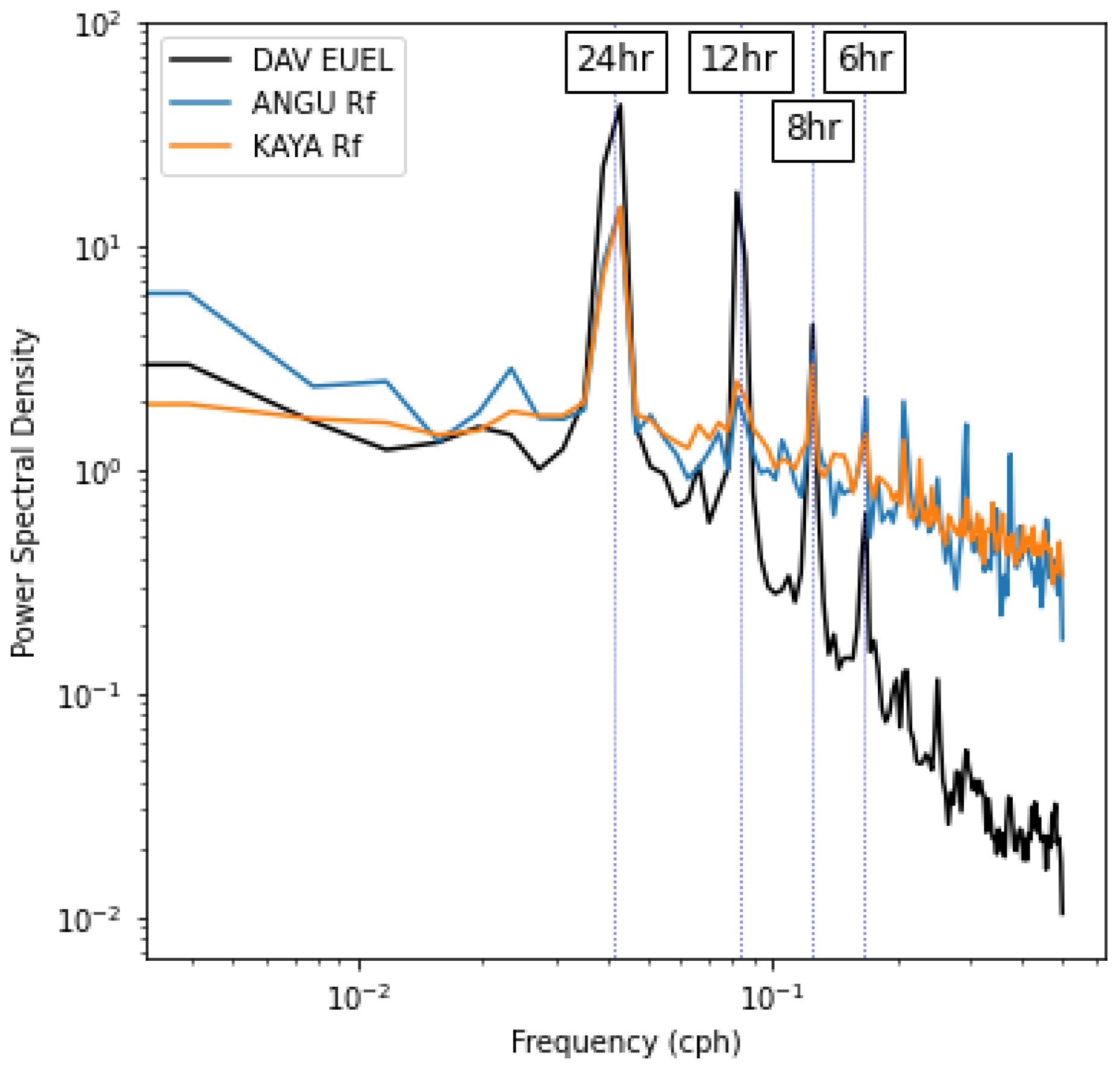
Over the full span of the timeseries analyzed, the daytime CNF-E feature was observed 39% and 41% of the day at ANGU and KAYA, respectively. The frequent observation of the CNF-E feature supports the likelihood that it is related to a persistent component such as the EEJ, and not due to transient phenomena such as sporadic E, which are relatively small patches of ionized plasma that occur at similar ranges to CNF-E and are observed with oceanographic HFR [11]. To further illustrate this, the power spectral density of the local EEJ magnitude given as EUEL at station DAV is compared to the power spectral density of the range to CNF-E feature (R_f) at ANGU and KAYA (Figure 8). Each of the power spectra show similar variability with strong peaks at 24-, 8- and 6- hour periods, and EUEL additionally shows a strong peak at 12-h period, while R_f at ANGU and KAYA show a weak peak at 12-h period. The similarity of power spectral density of the EUEL and R_f variables shows a strong relationship between diurnal geomagnetic effects of EEJ and a defining characteristic of the CNF-E feature.

The daily variability of the feature occurrences shown in Figure 8 exhibit a fair amount of short-term variability, with some longer-term trends visible. Power spectra density estimates were calculated for the daily averaged occurrence data (not shown), but no dominant signals were identified. It is of interest to understand if there is a relationship between the magnitude of the EEJ and the daytime noise feature. The occurrence of the CNF-E feature may be responsible for reduced performance of HFR radar by decrease SCNR at ranges past 90 km during the day. The minimum value of R_f is of particular importance to understanding the range of oceanographic HFR measurements, as is the count of daily occurrences which determines the temporal extent of the feature. Previous studies have used the daily maximum of the EUEL data as an indicator for localized EEJ strength [21], and correlation between the daily minimum of R_f and daily maximum EUEL and CNF-E and daily maximum EUEL are calculated at each site.

Table 3. Correlation Coefficient values between daily maximum value of EUEL and count of CNF-E feature occurrence and daily maximum value of EUEL and daily minimum R_f.

Correlation Coefficient Pair	ANGU	KAYA
Day maximum EUEL and Day minimum Rf	−0.05	−0.12
Day maximum EUEL and Day count CNF-E	−0.12	−0.04
Day value of F10.7 and Day minimum Rf	0.04	0.11
Day value of F10.7 and Day count CNF-E	−0.24	0.18
Day minimum EUEL and Day count of NF-Q	−0.04	−0.09
Day value of F10.7 and Day count of NF-Q	0.10	−0.22

shows that very low correlation exists between daily maximum EUEL and daily minimum R_f, and daily maximum EUEL and the count of CNF-E occurrences. Given the very weak correlation of C+NF features with geomagnetic fields, another set of correlation analysis is completed with F10.7 solar radio flux index. Table 3 also shows that there is also very weak correlation between the daily value of F10.7 and R_f and F10.7 and count of CNF-E occurrence. The lack of correlation between the CNF-E feature and its characteristic shape suggests that the HFR observations of the CNF-E feature may be influenced by upper atmospheric and ionospheric variability that is not captured by the magnetic and solar radio flux indices used here. Regardless of its origin, the CNF-E feature is a persistent feature of the HF propagation environment near the magnetic equator that ultimately effects the performance of backscatter signal retrieval from the ocean’s surface.

The nighttime NF-ARN feature was observed 35% and 30% of the day at ANGU and KAYA, respectively. The NF-ARN feature is similar to RFI and differs from clutter as elevated levels of noise are measured at all ranges recorded in the HFR backscatter spectrum. In general, RFI sources in the HF band consists of near and distinct lightning storms, local interference, and galactic sources. At 5 MHz, galactic noise is minimal [24], and the remote location of HFR sites does not support localized RFI. Ref. [6] produced global maps of the distribution of ARN from lightning, which show a maximum in ARN in the vicinity of Palau during the local nighttime hours. Additionally, satellite investigation of noise shows ARN strongest around equator and at night [25]. Thus, ARN is a likely source of noise as captured by the NF-ARN feature. Due to the complications of HF noise model that include lightning propagation [9], correlations between the NF-ARN feature and ARN are beyond the scope of this study.

Finally, the no-feature feature, NF-Q, is observed 14% and 21% of the time at ANGU and KAYA respectively. This feature is mostly observed in the time between observation of the CNF-E and NF-ARN features, which is around dawn and dusk. Previous studies have identified counter EEJ (CEJ) events that occur at dawn and dusk that result in a decrease in horizontal component of the earth’s magnetic field. Ref. [26] determined that CEJ is detected when EUEL value was below 5 nT for 2 h. In this study, EUEL values below 5 nT for 2 h were extracted and correlated with the occurrence of the NF-Q feature. As for the other C+NF features, there is weak correlation at both sites (Table 3). Another explanation for the NF-Q feature is that it is related to the NF-ARN feature which controls its occurrence. For example, if NF-ARN is weak during pre-dawn hours, a longer NF-Q will occur until the CNF-E feature builds around dawn.

Hour of Day Means

To understand the solar phase dependence of the propagation environment, hour of the day averages are created by separating the feature occurrence data into hourly bins and calculating the mean of each hour bin over the entire available timeseries. Figure 9 shows the hour of day mean occurrence of each feature, which exhibit similar variability at ANGU (Figure 9a–c) and KAYA (Figure 9d–f). As expected, the CNF-E feature (Figure 9a,d) has its highest occurrence during daytime hours, occurring over 80% at both ANGU and KAYA between 08:00 LT and 14:00 LT, with slightly higher peak values at ANGU. The NF-ARN feature (Figure 9b,e) is more frequent at ANGU, and occurrences are mostly observed between 17:00 LT and 07:00 LT with a peak at 21:00 LT. Conversely, the NF-Q feature (Figure 9c,f) is observed more frequently at KAYA, where both sites have a pre-dawn peak at 05:00 LT and a lower, pre-dusk peak at 16:00 LT.

In addition to the occurrence of C+NF features, the CNF-E feature characteristics (range to feature (R_f) and width of feature (W_r)) are compiled and hour-of day-means are computed (Figure 10). At both ANGU (Figure 10a) and KAYA (Figure 10c), R_f reaches a maximum around dawn (06:00 LT) and quickly heads to a minimum before noon (10:00 LT) while gradually returning to near maximum level at dusk (17:00 LT). The mean value at the 10:00 LT minimum is lower at KAYA, while larger standard deviation is observed at ANGU. Both sites also show similar diurnal variability in W_f (Figure 10b,d), which reaches a maximum at 09:00 LT, approximately 1 h before the minimum R_f is seen at both sites. W_f continues to decrease through the morning, and slightly increases towards afternoon to near maximum levels at 15:00 LT.

Similarly, hour of day means for the EUEL observations from DAV are calculated (Figure 11a) and show a peak occurring at 12:00 LT decreasing to near zero values at 0:00 LT. While there is general agreement between the EUEL and the occurrence of the CNF-E feature (Figure 9a,d), there are differences with the timing of the peaks. For example, the CNF-E feature peaks at 09:00 LT, where the EUEL peaks at 12:00 LT. The temporal variation of the hour of day EUEL mean (Figure 11b) shows a peak in rate of change of EUEL between 09:00 and 10:00 LT, around the same time that the CNF-E feature occurrences peak. This is also seen in the hour of day means of R_f and W_r (Figure 10), where R_f encounters a minimum at 10:00 LT and W_r reaches a maximum at 09:00 LT. Additionally, W_r at ANGU encounters an afternoon maximum at 15:00 LT which corresponds to the minimum in the rate of change of the EUEL hour-of-day means (Figure 11b).

4. Discussion

While designed and operated as a HF groundwave radar, backscatter collected during daytime hours from the CODAR Seasonde at our near-equatorial site in the Pacific exhibits a dependence on space weather conditions. The clutter at a range of 90–110 km from the radar which is a similar range to the bottom of the E layer of the ionosphere, peaks at mid-day and weakens with the solar sunset. Given the proximity of the Palau HFR observatory to the magnetic equator, there is likelihood that the daytime noise features are related to the Equatorial Electro Jet (EEJ), which is a narrow current of ionized particles centered around the magnetic equator that typically propagates eastward within the E layer of the ionosphere. The hour of day means (Figure 9 and Figure 10) reported in Section 3, offer a convenient way to characterize the general clutter + noise environment observed by HFR, which for the most part, exhibit similar variability and structure at both stations used in this study. Given these results, a general description of C+NF features occurring at the Palau HFR observatory follows: Preceding sunrise, C+NF levels are relatively low, and the C+NF no-feature feature NF-Q is observed between 20–40% of the time at 05:00 LT (Figure 10c,f). This time of day offers the best time for HFR oceanographic operations, as the RF environment supports high SCNR at extended range. As the sun rises, clutter in the ionospheric E layer is evident and occurrence of the CNF-E feature dominates the C+NF timeseries (Figure 10b,d). Initially, the feature range is observed at 115 km and width of 130 km at 06:00 LT, the feature width quickly increases to a maximum near 190 km at 09:00 LT while feature range quickly decreases to a minimum around 90 km at 10:00 LT. This corresponds with the maximum rate of change in the earth’s magnetic field observations associated with EEJ. As the day continues, the feature width decreases as feature range gradually increases to near maximum level around 110 km at 17:00 LT, and the CNF-E feature dissipates. Another short period of NF-Q feature between 16:00–18:00 LT is observed 20% of the time, followed by the nighttime feature NF-ARN that builds and peaks at 22:00 LT and continues throughout the night until it begins to dissipate around 05:00 LT. Unlike the CNF-E feature, the NF-ARN feature does not vary in range and is responsible for lowering SCNR through the entire operating range of the HFR, and often times precludes the measurement of ocean surface current completely.

There are strong similarities between the daytime feature, CNF-E, and the local EEJ index, EUEL, as both show variability at 24-, 8- and 6- cph frequencies (Figure 8). However, there is weak to no correlation between their daily compiled values (Table 3). This suggests that even though the CNF-E feature varies throughout the day with the EEJ, the intensity of the EEJ (as given by the daily maximum EUEL value) does not influence the CNF-E feature, as measured by the CODAR SeaSonde in its standard oceanographic setup. This suggests that oceanographic HF radars placed in proximity to the geomagnetic equator, may see range impacts under most geomagnetic conditions. Mitigation of the impacts will depend on further studies using vertically polarized antennas to provide calibrated vertical height measurements and specialized sensors for measuring ionospheric variability (digisonde, satellite, Radio Occultataion).

Design specifications for the 5 MHz band CODAR SeaSonde HFR used in this study specify observation ranges can extend to 200 km, a claim that is supported by the majority of SeaSonde HFRs in use. Clutter and/or RF noise is experienced at the sites in the Palau HF radar observatory for a majority of day. Given the persistence of the C+NF features, consistently achieving this range is not possible. HFR in all geographical locations observes clutter and noise that is often periodic, this is unavoidable given a crowded, shared-use RF spectrum and the increased range common in HF communications. However, most HFR with published results do not typically experience C+NF to the extent of the data presented in this study. The results presented here are important to consider when planning an ocean observation system that includes HFR. A simple solution would be to install more HFR to design around the 90 km range limitation during the daytime. The nighttime noise is far worse as far as the HFR data quality goes, and its mitigation is not as simple as deploying more HFR. Increasing HFR transmit power during the night may be a non-trivial engineering solution, however regulation of the RF spectrum restricts transmit power, and licensing high power in the lower HF frequencies can prove to be difficult. Some studies have looked at hardware solutions to suppressing HFR clutter, [27,28] and may be possible to implement into the CODAR SeaSonde HFR system.

While this study did not show strong correlation of the daytime C+NF feature with the EEJ, further investigation of this may be warranted as an alternative method to sensing the bottom of the ionosphere. Recent studies looking at coupled ionosphere and atmosphere models have shown complications with reproducing the variability below 200 km, due to simulations not being constrained by observations [29]. Additionally, the study showed that virtual height measurements at fixed frequencies are more impactful to reproduce the variations of the lower ionosphere as compared to parameters derived from traditional ionosphere sensing techniques (e.g., ionograms). There are a number of HFR in operation worldwide and finding a method to measure virtual height may provide an additional source of observations to improve these predictive models and our understanding of ionospheric variability.