Article

Real-Time Scan-to-Map Matching Localization System Based on Lightweight Pre-Built Occupancy High-Definition Map

1
GNSS Research Center, Wuhan University, Wuhan 430079, China
2
Intelligent Transport Systems Research Center, Wuhan University of Technology, Wuhan 430063, China
*
Author to whom correspondence should be addressed.
Remote Sens. 2023, 15(3), 595; https://doi.org/10.3390/rs15030595
Submission received: 3 October 2022 / Revised: 29 December 2022 / Accepted: 12 January 2023 / Published: 19 January 2023

Abstract

:
High-precision and robust localization in GNSS-denied areas is crucial for autonomous vehicles and robots. Most state-of-the-art localization methods are based on simultaneous localization and mapping (SLAM) with a camera or light detection and ranging (LiDAR). However, SLAM will suffer from drift during long-term running without loop closure or prior constraints. Lightweight, high-precision environmental maps have gradually become an indispensable part of future autonomous driving. In order to solve the problem of real-time global localization for autonomous vehicles and robots, we propose a precise and robust LiDAR localization system based on a pre-built, occupied high-definition (HD) map called the Extended QuadTree (EQT) map. It makes use of a planar quadtree for block division and a Z-sequence index structure within the block cells. Then, a four-level occupancy probability cell value model is adopted. It will save about eight times the storage space compared with Google Cartographer, and the EQT map can be extended to store other information. For efficient scan-to-map matching with our specialized EQT map, the Bursa linearized model is used in the Gauss–Newton iteration of our algorithm, which makes the calculation of partial derivatives fast. All the above improvements lead to optimal storage and efficient querying for real-time scan-to-map matching localization. Field tests in an industrial park and road environment prove that positioning accuracy of about 6–13 cm and attitude accuracy of about 0.15° were achieved using a VLP-16 LiDAR. They also show that the method proposed in this paper is significantly better than the NDT method. For the long and narrow environment of an underground mine tunnel, high-resolution maps are also helpful for accurate and robust localization.

1. Introduction

High-precision and robust localization is an extremely important task for autonomous vehicles and robots, as it is a prerequisite for autonomous vehicles and intelligent robots to perform the next task, such as path planning, obstacle avoidance, and so on [1]. Many researchers and companies have made great efforts to achieve high precision and reliable positioning in various complex scenarios.
Typically, the Global Navigation Satellite System (GNSS) and Inertial Navigation System (INS) are the most commonly used sensors to localize autonomous vehicles [2,3,4], as they are two kinds of sensors with good complementary properties. With the aid of differential signals, GNSS can provide absolute position without drift, and it is usually integrated with high-frequency relative pose information provided by INS for high-frequency and high-precision positioning. However, the GNSS/INS combination is not enough to meet the positioning needs of autonomous driving applications. GNSS signals are not always available, especially in urban areas with tall buildings and suffering from multi-path effects and signal block; furthermore, INS may suffer from boundless drift [5]. Except for the disadvantage mentioned above, GNSS/INS could only determine the position and orientation of the vehicle and could not perceive the environment around it.
To improve the accuracy and stability of vehicle positioning, onboard perceptual sensors such as the Light Detection and Ranging (LiDAR) sensor, monocular cameras, and stereo cameras have been adopted as solutions. Simultaneous localization and mapping (SLAM) as the state-of-the-art localization method is a promising way to solve the problem of vehicle positioning in certain scenarios; it enables a vehicle to calculate its position and orientation based on data obtained from onboard perceptual sensors. There are many open-source SLAM solutions, such as vision-based (the representative works are ORB-SLAM2 [6], ORB-SLAM3 [7], and VINS [8]) and LiDAR-based (the representative works are LOAM [9], Lego-LOAM [10], and LIO-SAM [11]), which all showed good positioning performance in complex environments. SLAM techniques have one major advantage: they can start working in any unfamiliar environment. However, SLAM will suffer from drift during long runs without loop closure constraints or prior constraints. Furthermore, it is unrealistic for vehicles to perform optimization based on loop closure constraints, as they cannot always go back to where they have been.
Another way to improve the accuracy and stability of vehicle positioning is to use a pre-built map, which could contain a lot of useful and precise environmental information. The core idea of localization in a pre-built map or map-based localization is matching: localization is the process of finding the best possible match between the onboard perceptual sensor data and the detailed information in the pre-built map [12,13]. High-precision map information can assist and enhance the robustness of positioning, which is an indispensable part of future autonomous driving. In the state-of-the-art approach, two different map structures are usually used: feature maps [14,15,16,17] and grid-occupied maps [18,19]. The most common method of map-based localization is to use the same onboard perceptual sensor for localization and mapping, as the same sensor has consistent characteristics. Compared with other perception sensors, LiDAR sensors have been widely used for environment perception as they have accurate range measurement capabilities and excellent performance in low light conditions. We chose LiDAR as the perceptual sensor for mapping and localization. Multi-sensor fusion is a popular solution to achieve the best performance of the positioning system and system redundancy, but in order to achieve true redundancy, these subsystems must also work independently to avoid dangerous situations caused by sensor failures. In this paper, we focus on LiDAR-only 6DOF localization based on a pre-built occupied map.
The main contributions of this paper are as follows: (1) We improved a novel pre-built 3D occupied HD map, which is called the Extended QuadTree (EQT) map, for scan-to-map matching in large areas. It utilizes a planar quadtree for block division and a Z-sequence index structure within the block cells. Additionally, for occupied cells, we adopted a four-level occupancy probability cell value model, which can save about eight times the amount of storage space and can accelerate querying the occupancy value from the map compared with Google Cartographer. (2) In our scan-to-map matching algorithm, the Bursa linearized model is applied in a Gauss–Newton iteration, which increases stability and accelerates positioning convergence, relying on our proposed special EQT map. (3) We have conducted extensive multi-scenario field tests to verify the reliability and accuracy of the method proposed in this paper. We also analyzed the impact of the EQT map resolution on positioning from a qualitative and quantitative perspective.
The remainder of this paper is constructed as follows: An overview of related works is represented in Section 2; the details of the LiDAR-only 6DOF localization method are represented in Section 3, including the construction of the EQT map and the Bursa linearized model in the Gauss–Newton algorithm; the field tests undertaken to evaluate the performance of the proposed method are presented in Section 4; and discussion, conclusions, and future work are presented in the remainder sections.

2. Related Works

The use of pre-built maps for localization has been studied in recent years, and some extensive algorithms have been proposed for autonomous vehicles and robots. For LiDAR sensors, there are two popular map structures: grid-based and feature-based. Most point cloud maps are two-dimensional and are projected from 3D point clouds, such as the orthographic reflectivity grid [13] and altitude map [16]. Feature-based maps can store feature information, such as colors, curvatures, semantic information, normals, or their combinations. Generally, map-based localization could be divided into two different approaches: point cloud scan matching and landmark searching [12,20,21].
Point cloud scan matching is the process of translating and rotating the online point cloud, which only contains a small area, around its center to match the larger prior point cloud map. The position and orientation relative to the prior map are calculated by satisfying some mathematical guidelines to make the best match between the online point cloud and the prior map. In the seminal work of Levinson et al. [13], they proposed an approach for high-precision positioning of moving vehicles using a high-resolution urban environmental map. The environmental grid map of reflectance intensity was generated offline by integrating GNSS, IMU, wheel odometry, and LiDAR data. A particle filter maintained a three-dimensional vector of 2D coordinates, and the yaw angle was used to match LiDAR measurements with the prior map. Then, they propose an extension of the above approach with less than 10cm RMS error; specifically, in order to better express the environmental information, they model the environment as probability models [18]. Wolcott, Ryan W., et al. [19,22] proposed a new scan matching algorithm using multiresolution Gaussian Mixture Maps (GMM), which is a two-dimensional grid data structure where each grid is modeled as a Gaussian mixture model. All online point clouds were used to align the GMM, and real-time performance was achieved through the development of novel branch-and-bound search and multiresolution approaches. Suzuki Taro et al. [23] described a method to estimate the 6-Degree of Freedom (DOF) position and attitude of mobile robots in an outdoor environment by using 3D point cloud data collected by the Mobile Mapping System (MMS); this method is based on the assumption that the mobile robots are always in contact with the ground. Wan Guowei et al. [24] present a localization framework to achieve reliable, high-precision positioning in various challenging environments. The framework integrates multiple complementary sensor information sources (LiDAR, IMU, GNSS) and involves a LiDAR global matching (LGM) positioning module relying on a pre-built map. LGM also acts as an important submodule to improve the accuracy and smoothness of positioning estimation in the work of Ding et al. [25]. LGM is a global localization method that matches the online point cloud against a pre-generated map to conduct a 3DOF (x, y, and yaw) scan. The pre-generated map is a grid-cell representation of the environment, and the statistics of LiDAR intensity and altitude are stored in each grid cell [25]. Iterative Closest Point (ICP) [26,27] and Normal Distribution Transform (NDT) [28,29] are the two most popular point cloud registration methods. In the ICP algorithm, an error metric between the source and target point clouds is minimized to iteratively optimize the transformation matrix. In the NDT algorithm, it is similar to ICP to iteratively optimize the transformation, but the error to be minimized is by first voting the target point cloud into grid cells and computing the probability density functions [21]. Through the work of N. Akai et al. [30] and M. Magnusson et al. [31], NDT was proven to be more robust than ICP. Valencia et al. [32] proposed an NDT-based Monte Carlo Localization (MCL) method that combined a constantly updated NDT occupancy grid short-term map with an offline static map; the short-term map was used only when the offline static map could not offer sufficient localization information. ICP and NDT point cloud registration methods could produce very accurate transformations between the source and target point clouds; however, it may be difficult for them in real-time applications.
Compared with the point cloud matching method, landmark searching is computationally less expensive, as it only uses a small number of online point clouds. Landmark search could perform excellent localization as long as there are enough landmarks in the environment. Alberto Hata et al. [33] proposed an improved road marking detector based on the OTSU threshold method to segment the point cloud into asphalt and roads, then vehicle localization is achieved by aligning the road markers and curbs to the pre-built 3D map. Kim et al. [34] proposed an approach to lane marker map building and localization for autonomous vehicles by using a 2D laser rangefinder. Lane markers were detected from reflectivity values as local features, and the localization algorithm is based on the point-to-plane ICP algorithm. Farouk Ghallabi et al. [35] proposed a method to solve the positioning problem by matching the road perception information of the 3D LiDAR sensor with the HD map elements; specifically, the particle filter algorithm is used to match the observed High Reflective Landmarks (HRL) with HD map elements to estimate the position of the vehicle. Jeong et al. [36] use an onboard stereo camera and HD map to achieve 6-DOF pose estimation in an urban environment; their HD map stores 3D geometric data with semantic information expressed in a compressed format.

3. Methodology

The proposed LiDAR-based 6DOF localization method in this paper relies on a pre-built 3D point cloud map; our goal is to solve the problem of continuous and reliable positioning in a GNSS-denied environment. The pre-built map is a volumetric (voxel) representation of the environment; each voxel stores a value representing the probability of being occupied [37]. We achieve 6DOF pose estimation by matching the online point cloud scan with the pre-built map, and the initial pose of the scan is continuously optimized through the Gauss–Newton iteration method.

3.1. Map Generation

One key challenge to achieving rapid map-based localization is building a prior representation of the world (modeling the 3D environment) [18], modeling the areas of free, occupied, and unmapped space, and importantly, ensuring that access times and memory consumption are efficient. In the field of robotics and SLAM, there have been several environmental models used in practice, such as point clouds, elevation maps, multi-level surface maps, and semantic maps. A point cloud is not memory efficient, as it would consume a large amount of memory to store points. An elevation map and multi-level surface map are memory efficient, but they could not model the area that was unmapped and lack the ability to model any 3D environment. In this paper, we use an occupancy grid map for environment representation that is similar to OctoMap [37]. The occupied grid map divides the environment into a series of grids, and each grid is assigned a probability value between 0 and 1. The probability value indicates the probability that this grid is occupied. The occupied grid map is widely used because of its convenience in creation and maintenance. It is especially suitable for processing laser or ultrasonic measurement data.
The state of each grid in the occupancy grid map is not a “black” or “white” state but is represented by the probability that the grid is occupied by obstacles. Let p s = 0 indicate the probability of a grid being occupied and p s = 1 indicate a grid being free; they satisfy p s = 0 + p s = 1 = 1 . In actual application, the state of a grid was computed as O d d s = p s = 1 p s = 0 for convenience. The state of the grid in the occupancy grid map needs to be constantly updated when new point clouds are inserted into the map. The probability of a grid being occupied will be updated according to (1) when given the sensor measurement z ~ 0 , 1 .
O d d s z = p s = 1 z p s = 0 z
According to Bayesian formula, we can get:
p s = 1 z = p z s = 1 p s = 1 p z p s = 0 z = p z s = 0 p s = 0 p z
Further, we can get a new state update (3) by taking the logarithm of the map grid state.
log O d d s z = log p z s = 1 p z s = 0 + log O d d s
For log O d d s z update, it will be faster than O d d s z as multiplications are replaced by additions. log p z s = 1 p z s = 0 is called a measurement module, which has two forms:
lofree = log p z = 0 s = 1 p z = 0 s = 0 looccu = log p z = 1 s = 1 p z = 1 s = 0
It is convenient to convert log O d d s z into probability and vice versa; therefore, log O d d s z is stored in the occupancy grid map instead of the occupancy probability. In the state-of-the-art work of Google Cartographer [38], the minimum and maximum occupancy probability values are mapped to the integer interval [1,32767]. To reduce the amount of floating-point calculations, it means that the occupation probability value is divided into 32,767 levels, and storing an occupancy probability value will consume 16 bits of memory. To further reduce memory consumption, a simplified occupancy probability value mapping model is used in this paper. We divided the occupancy probability value evenly into four levels, which means that storing an occupancy probability value will only consume 2 bits of memory. For a single float value (usually 4 bytes), one could only store 1 occupancy probability value (2 bytes for index and 2 bytes for occupancy probability values) when using Google’s method, and a single float value could store 8 occupancy probability values (2 bytes for index and 2 bytes for 8 occupancy probability values) when using our method.
The octree data structure is used to store maps for flexible storage and application of map data and is a tree-like data structure used to describe a three-dimensional space. While the typical octree index structure will consume a lot of computing resources for spatial data queries, it is not suitable for real-time map matching. Therefore, considering the sparse characteristic of the point cloud, we simplify the index structure of voxels for quick queries. Specifically, we first divide and calculate the index items according to the ground plane in the horizontal direction, which are stored in a planar quadtree; thus, we can quickly query and locate the position of the planar voxel through the planar quadtree; after location to the planar quadnode, we divide and calculate the linear index along the elevation direction (Z axis direction), which are stored in a linked list structure. Each voxel only stores the occupancy probability information; in fact, each voxel can be further expanded to store more information, such as light intensity, semantics, and other information. In addition, the quadtree structure allows us to obtain multiple resolution maps by limiting the depth of the querying; thus, we can achieve coarse-to-fine matching in the scan-to-map matching stage. The high-precision voxel map model based on a planar quadtree and elevation index is shown in Figure 1.
In general, our point cloud map uses a planar quadtree for block division and a Z-sequence index structure within the block. A four-level mapping occupancy probability value model is also adopted. All the efforts lead to optimal storage and query efficiency for real-time scan-to-map matching positioning.

3.2. Scan-to-Map Matching

Taking the mechanical drive mechanism of the VLP-16 lidar we used into account, it may take several milliseconds to acquire a complete scan. In this process, the continuous movement of the sensor will cause point cloud distortion. Thanks to our high-precision hardware time synchronization, the precise sampling time of each point can be accurately obtained. We eliminate the distortion of the original laser scanning by transforming each point to the same time based on the assumption of a uniform motion model [39]. The scan-to-map matching module needs to be initialized with roughly accurate initial pose estimation. Generally, we could get the initial pose from a GNSS receiver or inversely calculate it from known landmarks. Then, the online point cloud scan obtained from LiDAR can be matched with the pre-built HD map continuously. The main goal of scan-to-map matching is to find rigid transformation parameters that make the best match between the online scan and the pre-built map. Here we try to estimate the rigid transformation parameters that minimize the residual of the occupation probability value. The problem of scan-to-map matching can be modeled as a nonlinear least squares problem, which can be expressed as:
ξ * = arg min ξ i = 1 n 1 M ( S i ( ξ ) ) 2
where ξ = x , y , z , r o l l , p i t c h , y a w T is the 6DOF pose to be optimized from the current scan, n is the point number of the scan, S i ξ means transform a point in a LiDAR frame to a map coordinate frame, as in (2), and M S i ξ will return the occupancy probability value of point S i ξ on the map.
s i ( ξ ) = R r o l l , p i t c h , y a w s i , x s i , y s i , z + x y z
In this paper, we choose the Gauss–Newton iteration method to solve (5) for pose optimization. It is an iterative method for finding regression parameters for least squares in a nonlinear regression model. This method uses Taylor series expansion to approximately replace the nonlinear regression model, and then through multiple iterations to modify the regression coefficients, the regression coefficients are constantly approaching the best regression coefficients of the nonlinear regression model, finally minimizing the sum of residual squares. With an initial pose estimation ξ 0 = x 0 , y 0 , z 0 , r o l l 0 , p i t c h 0 , y a w 0 T of ξ = x , y , z , r o l l , p i t c h , y a w T , we try to find an optimal pose change Δ ξ that makes the current point cloud projected on the pre-build map to get the smallest occupancy probability residual value:
i = 1 n 1 M ( S i ( ξ + Δ ξ ) ) 2 0
According to the Taylor series formulation, expand M ( S i ( ξ + Δ ξ ) ) at ξ = x , y , z , r o l l , p i t c h , y a w T to get:
i = 1 n 1 M ( S i ( ξ ) ) M ( S i ( ξ ) ) S i ( ξ ) ξ Δ ξ 2 0
If Δ ξ makes (8) achieve the minimum, we can get (9):
2 i = 1 n M ( S i ( ξ ) ) S i ( ξ ) ξ T 1 M ( S i ( ξ ) ) M ( S i ( ξ ) ) S i ( ξ ) ξ Δ ξ = 0
Thus, we can solve (9) to get Δ ξ :
Δ ξ = H 1 i = 1 n M ( S i ( ξ ) ) S i ( ξ ) ξ T 1 M ( S i ( ξ ) )
where M S i ( ξ ) means the gradient of the map occupancy probability value, and H is called the Hessian matrix, which is expressed as:
H = M ( S i ( ξ ) ) S i ( ξ ) ξ T M ( S i ( ξ ) ) S i ( ξ ) ξ
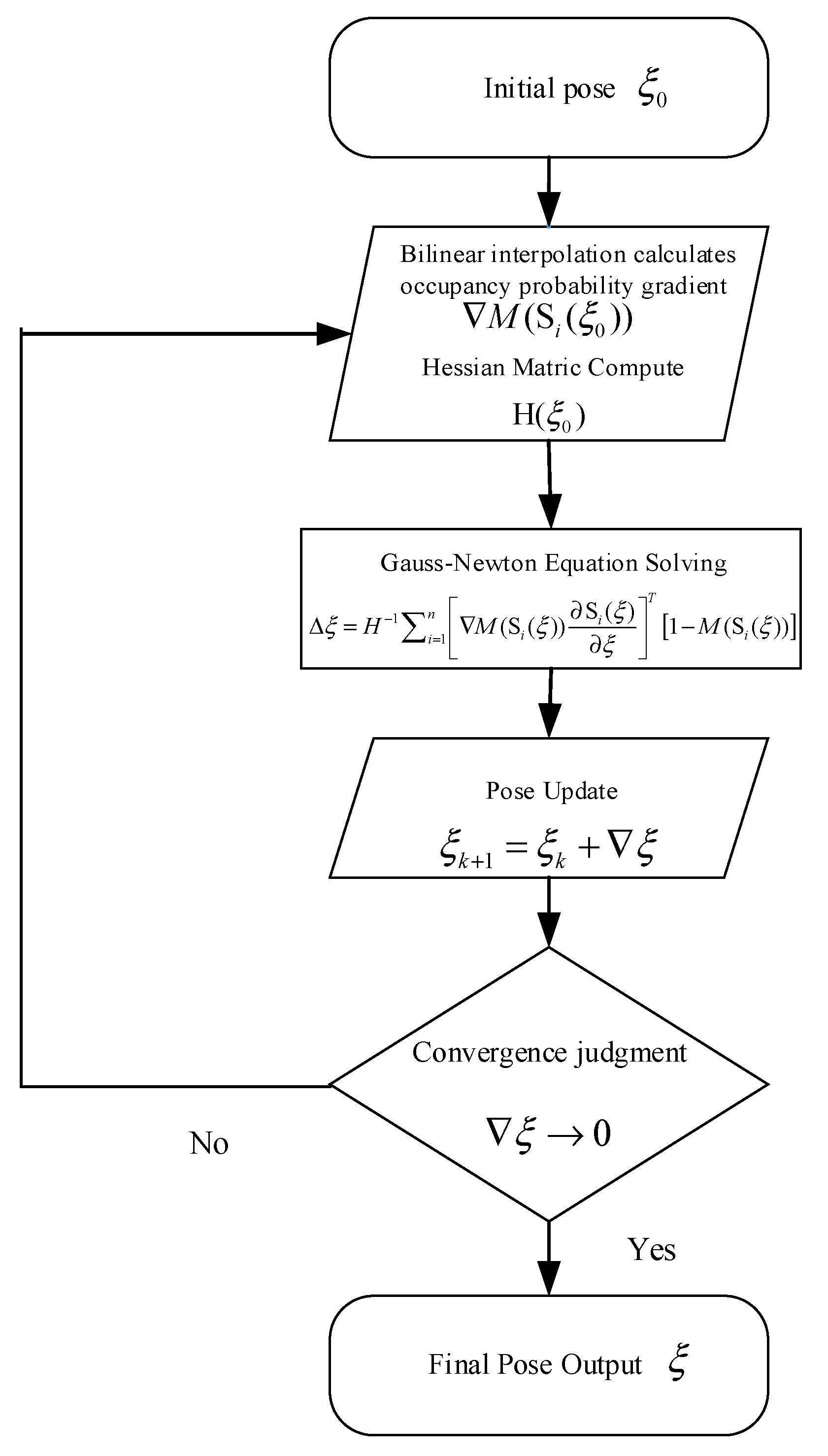
The whole procedure of scan-to-map matching for localization is presented as follows in Figure 2.
In the above Gauss–Newton iteration algorithm, the most important thing is to calculate the partial derivative of the pose S i ( ξ ) ξ and the probability gradient M S i ( ξ ) . In the process of obtaining the partial derivative of the pose, we adopted the Bursa simplification strategy in the linearization process. When the Euler angles in the pose parameter ξ = x , y , z , r o l l , p i t c h , y a w T are small, we can get a simplified coordinate transformation formula without considering the scale parameter in Bursa’s six parameters shown in (12), and we can obtain the derivative directly without interpolating like Google Cartographer.
X 2 Y 2 Z 2 = 1 y a w p i t c h y a w 1 r o l l p i t c h r o l l 1 X 1 Y 1 Z 1 + x y z

4. Experiment and Result

4.1. Platforms

The performance of localization based on a pre-built HD map presented in this paper was tested and verified in a variety of different scenarios, including an industrial park, a city road, and an underground mine tunnel. MMS was used for collecting HD maps of the industrial park and road environment because there are good GNSS signals, and maps of underground mines were collected by Terrestrial Laser Scanning (TLS) and vice versa. The VLP-16 LiDAR and Honeywell HG4930 IMU were integrated with a high-precision GNSS board; the MMS built in this paper is shown in Figure 3. The specific performance parameters of the HG4930 IMU are shown in Table 1. The VLP16 LiDAR and IMU were strictly time synchronized through the pulse per second (PPS) signal output by GNSS. The VLP16 LiDAR worked at a frequency of 10 Hz, the sampling rate of GNSS was 1Hz, and the IMU worked at a high frequency of 600 Hz.
GNSS Real Time Kinematic (RTK) is a widely used positioning technology that eliminates or weakens most of the errors (such as orbital error, clock error, ionospheric delay, tropospheric delay, etc.) through differential signals. GNSS RTK/INS can not only further improve positioning accuracy and robustness but also obtain attitude information. In the point cloud map generation phase, the GNSS RTK/INS smoothing integration result was used to stitch continuous multi-frame point clouds to generate point cloud maps. While GNSS signals are not available in underground mine spaces, we used the FARO Laser Scanner Focus 3D X330 for environmental point cloud collection. The FARO Laser Scanner Focus 3D X330 is a sophisticated measuring device that can produce a high-precision and high-resolution point cloud. In the data acquisition stage, a common-view target ball was placed between the measuring stations, and in the data processing stage, multiple stations were spliced to generate a complete point cloud.
Our test scenes were divided into two categories: one was an open-sky area with good GNSS signals, and the other was a GNSS-denied scene. We carefully quantitatively evaluated and analyzed the performance of our proposed algorithm, including RMS, maximum positioning error, maximum attitude error, and cost time. The algorithm ran on a modern laptop, which is an Intel(R) Core (TM) i7-7700HQ at 2.8GHz and 16.0 GB of RAM. In order to verify the performance of the algorithm proposed in this paper, we compared it with the traditional NDT method.

4.2. Industrial Park and Road Environments

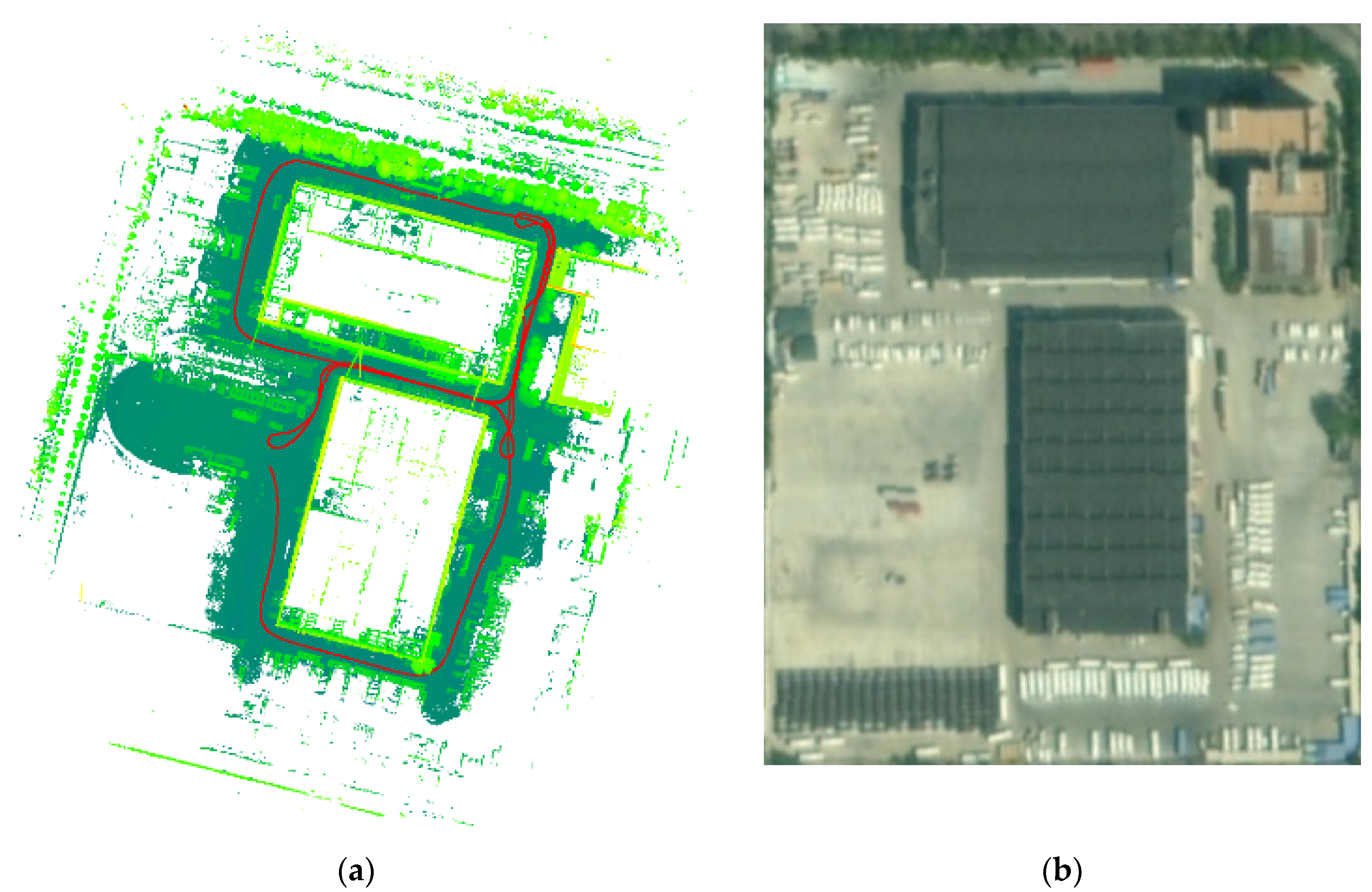
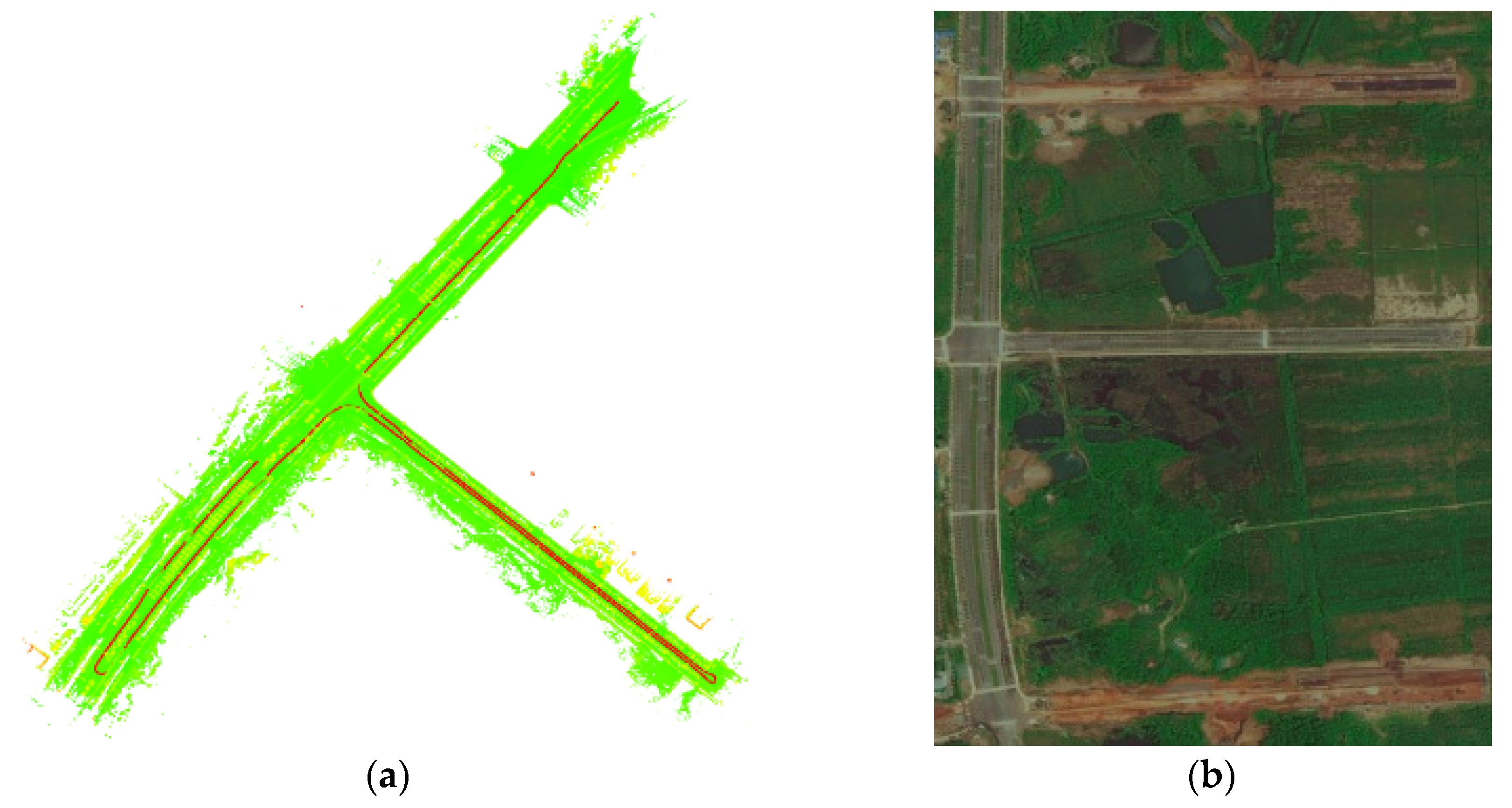
We first conducted experiments in industrial parks and on urban roads. The two-way smoothing trajectory of the GNSS RTK/INS integrated navigation was utilized to split multiple frames of continuous point clouds into a point cloud map. Firstly, we collected a set of synchronized GNSS, IMU, and LiDAR data to generate the pre-built EQT HD map, in which we manually removed dynamic objects so that only static objects remained on the map. The pre-built EQT maps and experimental site environments are shown in Figure 4 and Figure 5. The red line on the map is the reference trajectory provided by the GNSS RTK/INS smoothing integration algorithm. During the field test, the average speed of the vehicle was about 25km/h.
We used commercially integrated navigation software, GINS, to calculate the reference groundtruth. GINS can provide information such as the number of available satellites and dilution of precision (DOP) value, which indicate the quality of the GNSS observation environment. The number of available satellites and DOP values in the industrial park environment and the road environment are shown in Figure 6 and Figure 7. We can find that the number of available GNSS satellites in the industrial park environment is obviously less than that in the road environment, and the DOP value in the industrial park environment is obviously larger than that in the road environment. It shows that the observation conditions for GNSS in the road environment were obviously better than those in the industrial park environment.
The file size of the pre-built map is an important factor in practical applications, as it may affect the efficiency of the scan matching algorithm. More importantly, in the high-precision positioning map service for future autonomous driving, map data files must be placed on the cloud server first, so that the smaller the amount of map data, the better the map data transmission. The resolution of the map mainly determines the size of the memory occupied by the map. The shape of the industrial park is rectangular, and its area is about 250 m × 250 m. The road test environment includes 1.6 km of roads with essentially no tall buildings on either side. We constructed point cloud maps for testing industrial parks and road scenes with resolutions of 8 cm, 16 cm, and 24 cm. The NDT algorithm uses a PCD file as input, and the file sizes of the EQT map with different resolutions and the PCD file are shown in Table 2. It is shown that according to our map construction method, when the resolution changes from 8 cm to 16 cm or 24 cm, the map memory consumption of the industrial park is reduced by 77.9% and 90.3%, respectively, and the map memory consumption of the roads is reduced by 74.5% and 87.9%, respectively. The PCD file used in the NDT algorithm is much larger than the EQT map.
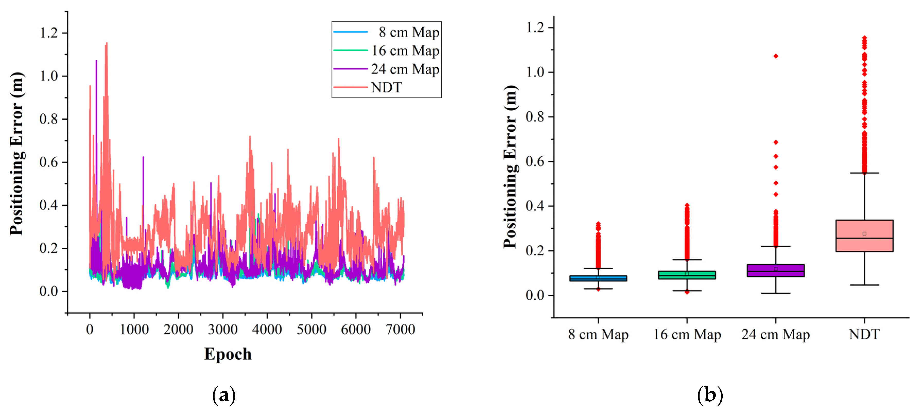
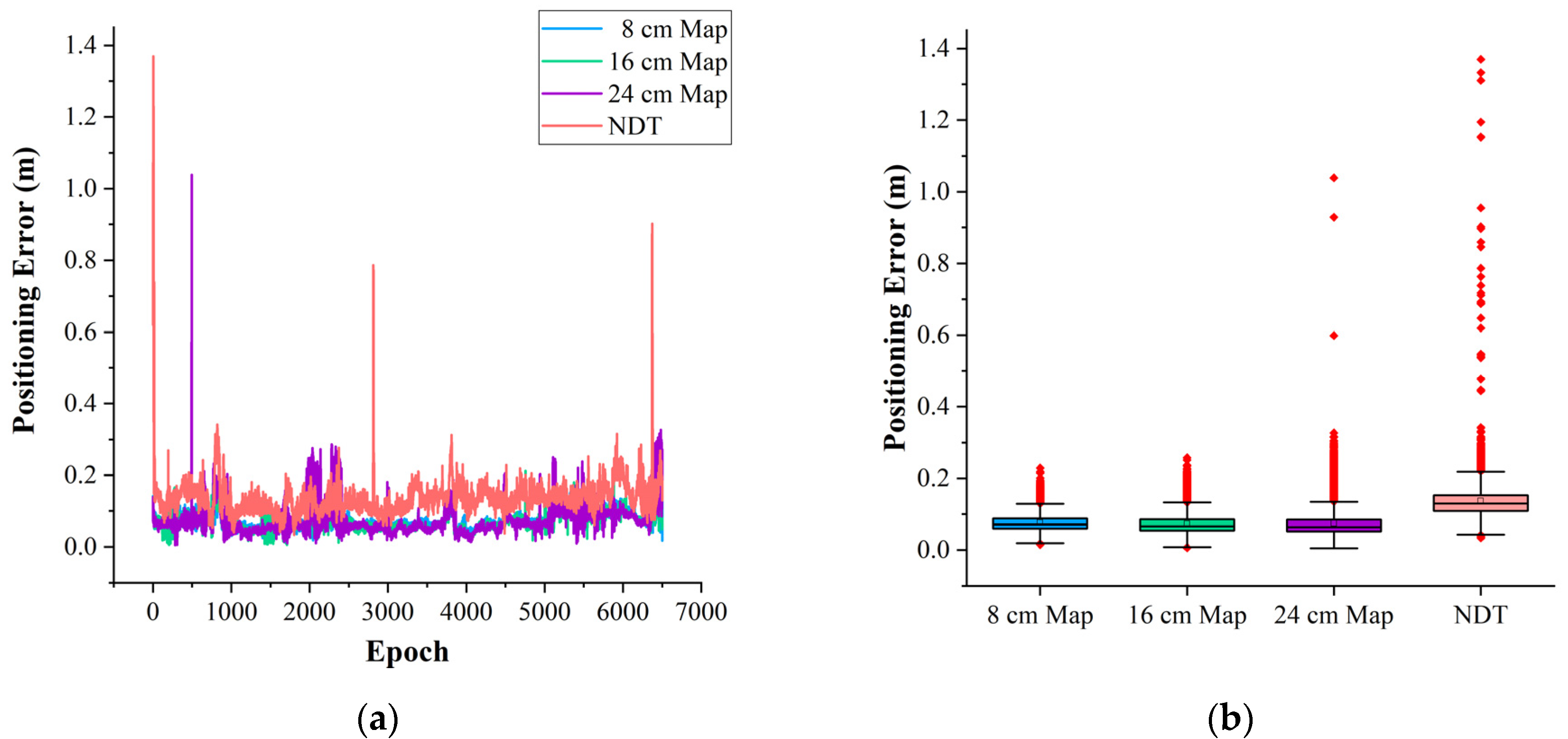
The localization performance based on the EQT map of different resolutions and the NDT match are shown in Figure 8 and Figure 9. As can be seen from Figure 8 and Figure 9, the localization performance of the method proposed in this paper is better than the NDT algorithm. We have detailed statistics on the distribution of position error and attitude error, as shown in Table 3 and Table 4. In the field test of an industrial park, the RMS of positioning error is 0.085 m and the RMS of yaw error is 0.162° when the resolution of the pre-built EQT map is 8 cm; the RMS of positioning error is 0.105 m and the RMS of yaw error is 0.163° when the resolution of the pre-built EQT map is 16 cm; the RMS of positioning error is 0.129 m and the RMS of yaw error is 0.146° when the resolution of the pre-built EQT map is 24 cm; and the RMS of positioning error is 0.301 m and the RMS of yaw error is 0.519° when using the NDT algorithm. In the field test of roads, the RMS of positioning error is 0.077 m and the RMS of yaw error is 0.132° when the resolution is 8 cm; the RMS of positioning error is 0.076 m and the RMS of yaw error is 0.138° when the resolution is 16cm; the RMS of positioning error is 0.090 m and the RMS of yaw error is 0.130° when the resolution is 24 cm; and the RMS of positioning error is 0.148 m and the RMS of yaw error is 0.134° when using the NDT algorithm.
The percentages of scans where the matching algorithm achieves positioning better than 0.1 m, 0.2 m, or 0.3 m and calculating attitude accuracy better than 0.1°, 0.2°, or 0.3° are shown in Table 5 and Table 6, and maximum positioning errors are also presented. It can be seen that as the resolution increases from 8 cm to 24 cm, the probability of large errors increases significantly, especially in the field test of the industrial park, where the percentages of positioning achieving better than 0.1 m are 85.39%, 67.76%, and 42.00%, respectively. It can also be seen from Table 3 that the change in resolution has a smaller impact on positioning performance in the field test of an industrial park than in road environments.
The time cost was calculated to verify the efficiency of the proposed positioning method based on a pre-built map. The statistical average time cost is shown in Table 7. We can find that the average time cost has a slight decreasing trend when the resolution of the pre-built map changes from 8 cm to 24 cm. The average time cost of each scan match is far less than the frame rate (100 ms) of LiDAR, which verified the efficiency of our algorithm and can be used for real-time positioning. From Table 7, we can also see that the method proposed in this paper is more computationally efficient than the NDT algorithm.

4.3. Underground Mine Tunnel Environment Experiment

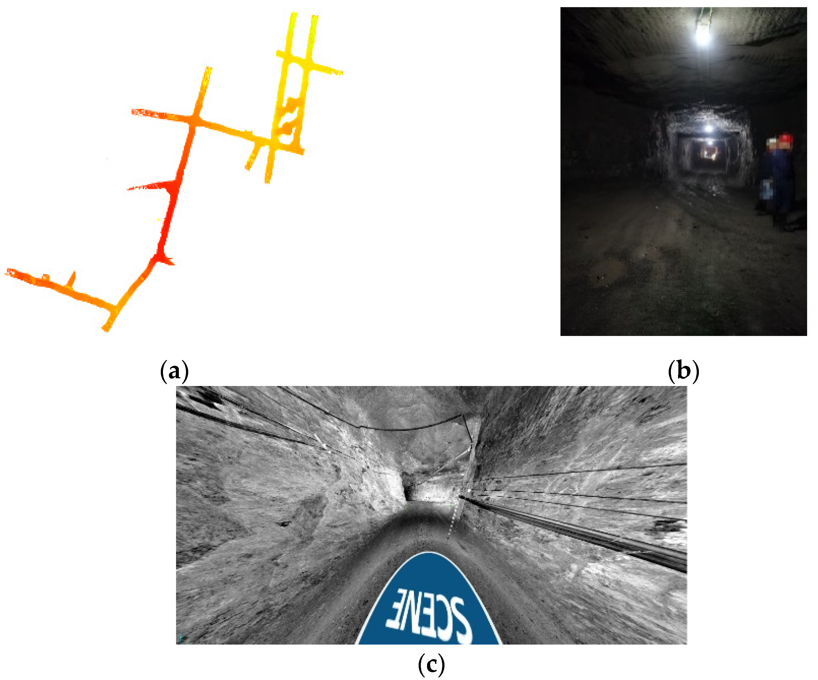
We also evaluated the positioning performance of our algorithm in an underground mine tunnel environment. The road in the mine tunnel is rugged, with uphill and downhill sections. Since commonly used MMS cannot be used to collect point cloud maps in GNSS-denied environments such as underground mines, the FARO Laser Scanner Focus 3D X330 was used to collect point clouds to construct QET maps. The pre-built point cloud map and real underground mine tunnel environment are shown in Figure 10. The mine tunnel is about 5 m wide and 4.5 m high. We also used the vehicle-mounted VLP-16 LiDAR for positioning data collection, and the length of the test path is about 600 m. Due to the lack of groundtruth, we only performed a qualitative analysis on the positioning results. Due to the complex environment under the mine, the average speed of the vehicle was 10 km/h during the field test.
We constructed point cloud maps for underground mine tunnels with resolutions of 8 cm, 16 cm, and 24 cm; the file sizes of the EQT maps of different resolutions are shown in Table 8. From Table 8, we can see that according to the point cloud map construction method in this paper, when the resolution changed from 8 cm to 16 cm and 24 cm, the map memory consumption was reduced by 68.7% and 76.2%, respectively. The PCD file used in the NDT algorithm is also much larger than the EQT map.
The positioning trajectories in the underground mine tunnel are shown in (a) of Figure 11, and the XYZ view is shown in b of Figure 11. The positioning trajectories based on the EQT maps of 8 cm, 16 cm, 24 cm resolution, and NDT trajectory are respectively marked as Traj_A, Traj_B, Traj_C, and Traj_NDT. It is obvious that Traj_NDT ends up in chaos, which indicates that the NDT algorithm failed at last. The trajectories inside the red ellipse in (a) of Figure 11 are enlarged and shown in (c) of Figure 11. As it can be seen from (b) of Figure 11, the differences between Traj_A, Traj_B, and Traj_C are very small except for the red box in (b) of Figure 11; the trajectories in the red box are enlarged and shown in (d) of Figure 11. It is obvious that the Traj_B and Traj_C were wrongly positioned, as the vehicle-mounted VLP-16 LiDAR was essentially moving at a constant speed during the field test. From (d) of Figure 11, we can also see that Traj_A was smoother than Traj_NDT. At the same time, we carefully checked the point cloud data used to build the map. The point cloud map in the NDT location failure part is complete, so the failed NDT algorithm trajectories are not related to defects in the construction of the map.
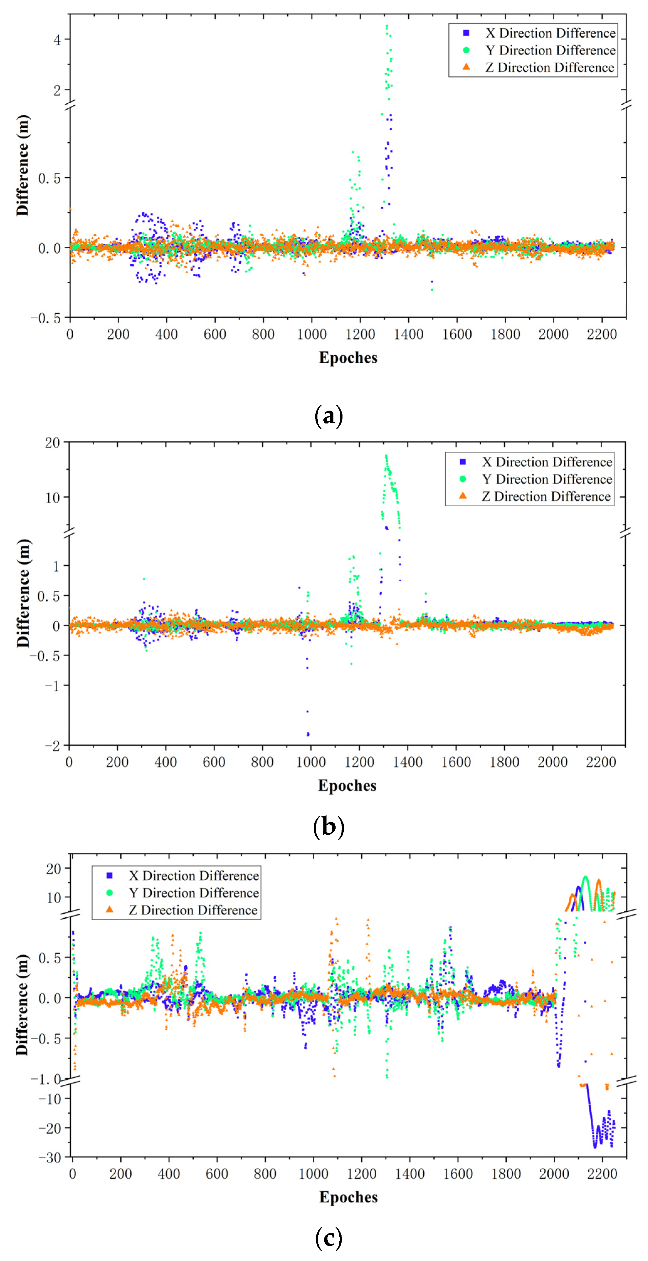
We further compared and analyzed the differences between Traj_A, Traj_B, Traj_C, and Traj_NDT in detail. Due to the complex environment under the mine, there is no groundtruth that can be referenced, so we take Traj_A as a reference for qualitative analysis because Traj_A was the smoothest of the four trajectories. The difference between Traj_A and Traj_B, Traj_A and Traj_C, and Traj_A and Traj_NDT in the same epoch is shown in Figure 12 for each. Among the differences between Traj_A and Traj_B in the X, Y, and Z directions, the percentages of difference less than 0.1 m are 93.6%, 96.4%, and 97.3%. Among the differences between Traj_A and Traj_C in the X, Y, and Z directions, the percentages of difference less than 0.1 m are 89.1%, 91.2%, and 90.2%. The biggest difference between Traj_A and Traj_B can reach 4.5 m in the Y direction, and the biggest difference between Traj_A and Traj_C can reach 17.5m in the Y direction. We can see from (a),(b) of Figure 12 that they were essentially in the same place. Although it is obvious that there is a large positioning error in Traj_B and Traj_C, we can see a convergence process in (a), (b) of Figure 12; it converged to the correct position through subsequent epochs. From one aspect, it reflects that our algorithm can tolerate large initial position errors in an underground mine tunnel environment. While among the differences between Traj_A and Traj_NDT in X, Y, and Z directions, the percentages of difference less than 0.1 m are 64.7%, 64.3%, and 71.2%. Traj_A and Traj_NDT have large errors in the last part because Traj_NDT was wrongly positioned at the end.
The statistical average time cost of scan-to-map matching is shown in Table 9. It seems that the average time cost of using maps with different resolutions makes no difference. The average time cost in the field test of an underground mine tunnel was less than in the field test of an industrial park or road environment, which may have been caused by the long and narrow environmental characteristics of the underground mine tunnel. It also indicates that the method proposed in this paper is more computationally efficient than the NDT algorithm.
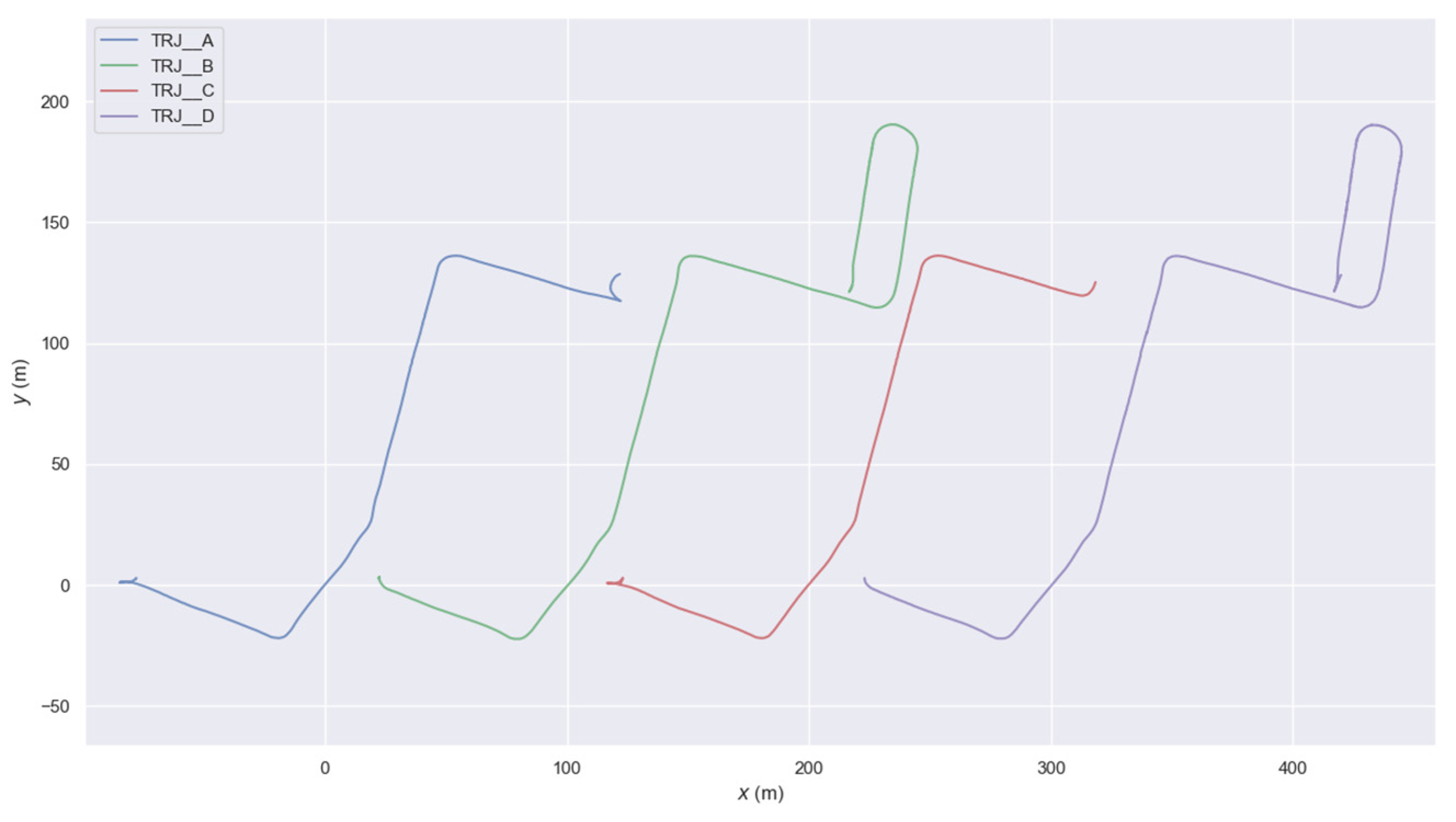
We conducted four data collections according to the mining route, including two complete routes from the ore loading point to the ore unloading point and two complete routes from the ore unloading point to the ore loading point. We used the EQT map with a resolution of 8 cm for vehicle positioning; the trajectories are shown in Figure 13. Although there is no groundtruth, we can see that our four trajectories were continuous and complete, which can prove the stability of our algorithm to a certain extent.

4.4. KITTI Dataset

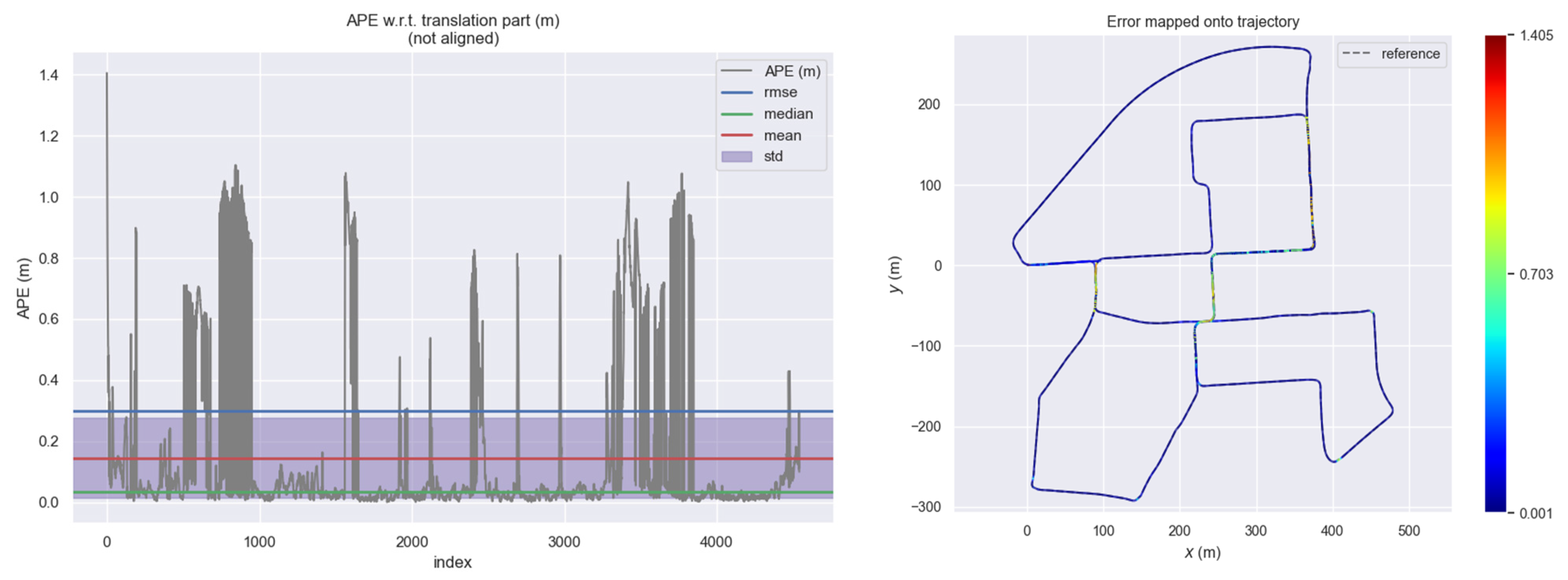
The KITTI dataset was jointly established by the Karlsruhe Institute of Technology in Germany and the Toyota American Institute of Technology. It is the world’s largest and most popular dataset for automatic driving and SLAM technology evaluation. First, we used the groundtruth provided by the KITTI dataset to splice all point cloud frames into a complete point cloud map and then used our method to generate an EQT map; all maps used 15 cm resolution. Then, we gave an initial pose to achieve continuous positioning of point cloud frames. The initial pose was based on the truth value, which added 0–20.0 cm of random error to the position and 0–1.0 degree of random error to the pose. Before the calculation, the point cloud of each frame was uniformly downsampled, and about 10,000 points were reserved for each frame. Then, we used the SLAM evo [40] tool to evaluate the absolute position error (APE) and count the error information. Evo is a trajectory evaluation tool for odometer and SLAM problems. Its core function is to be able to draw the groundtruth, or evaluate the error between the trajectory and the groundtruth in formats supporting multiple data sets. We counted the maximum, average, root mean square error (RMSE), and standard deviation (STD) of the absolute position error of each group of data sets, as well as the average time cost (ATC) of each frame; the results are shown in Table 10. It can be seen from Table 10 that most of the absolute positioning accuracy of our method is very high, achieving centimeter-level positioning.
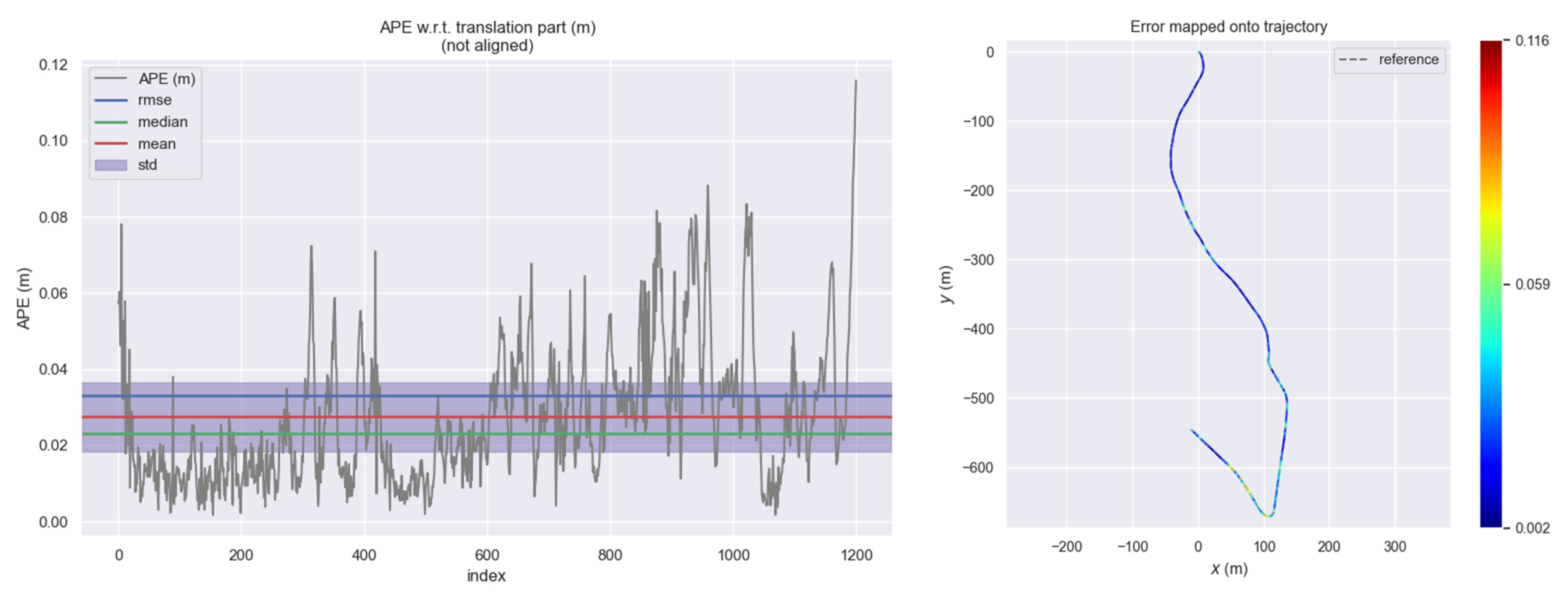
The positioning results of datasets 00 and 08 are poor, dataset 10 is the best. Figure 14 and Figure 15 show the APE results and trajectories of datasets 00 and 10. From Figure 14, we can find that the reason for the poor statistical results of data set 00 is that there are a large number of large positioning errors in the repeated track sections. We think that the possible reason for this phenomenon is the inaccuracy of the two trajectories, which leads to the inaccurate stitching of the prior point cloud map. We do find that in the groundtruth, there is sometimes a large error in the Z-direction, which will cause the map to be inaccurate. Although we use the same set of data to build maps and locate, this can also show the high accuracy of our location algorithm. We have to admit that there is a risk of positioning failure when the map environment changes greatly.

4.5. Ablation Study

In order to verify the improvement in computing efficiency brought by the Bursa model, we carried out experimental verification on the KITTI dataset 09. The Bursa seven-parameters model is a model commonly used in geodesy to solve the problem of coordinate conversion parameters between two rectangular coordinate systems; of course, we have not considered the scale factor here. The Bursa parameters model removes the linearized high-order terms based on the small angle vacation to simplify calculation. If we rotate the point according to three Euler angles between two coordinate systems, the rotation matrix is:
R = cos ε y cos ε z cos ε y sin ε z sin ε y cos ε x sin ε z + sin ε x sin ε y cos ε z cos ε x cos ε z + sin ε x sin ε y sin ε z sin ε x cos ε y sin ε x sin ε z + cos ε x sin ε y cos ε z sin ε x cos ε z + cos ε x sin ε y sin ε z cos ε x cos ε y
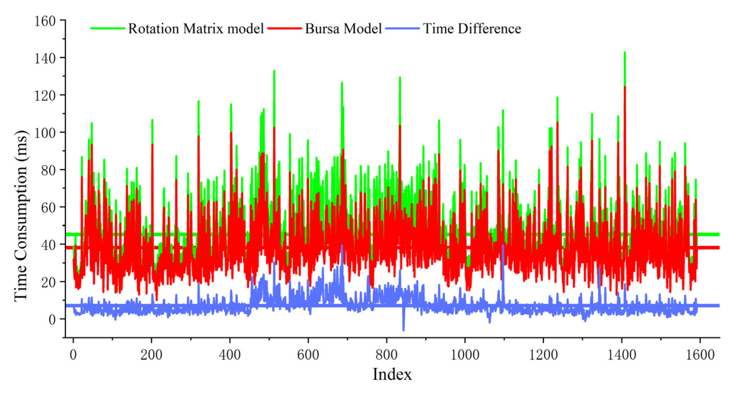
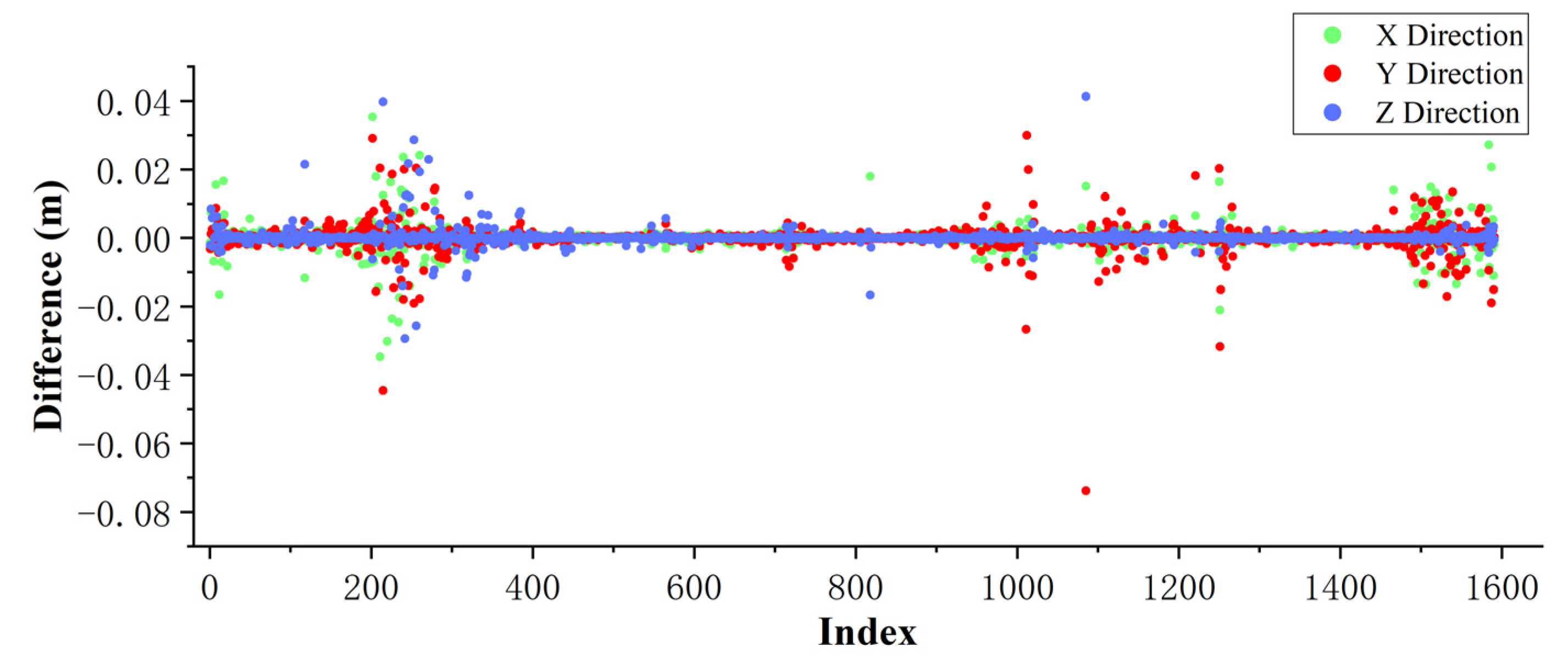
If the form of a rotation matrix is used to solve the partial derivative H-matrix, the formula will be complex; although this calculation is not very large for the computer, each point needs to be calculated once for each iteration. We used the Bursa model and the rotation matrix model to simulate and calculate the partial derivative H matrix 10,000 times. The Bursa model hardly consumes time, and the rotation matrix would take about 1ms. Then we used the Bursa model and the rotation matrix model to calculate the 09 data of KITTI data; the calculation time and positioning result difference of each frame are shown in Figure 16. The average calculation time for using the Bursa model is 38.1 ms, and the average calculation time for using the rotation matrix is 45.2 ms. The average time consumption of using the Bursa model is reduced by 7.1 ms, which is 15.7%. From Figure 17, we can see that the positioning results of the two models are almost the same, so using the Bursa model will increase calculation efficiency without sacrificing accuracy.

5. Discussion

To evaluate the positioning performance of the method proposed in this paper, extensive field tests for different scenarios have been conducted. From the field test in industrial parks and road environments, the positioning accuracy was mostly consistent with the reference trajectory calculated by the GNSS RTK/INS integrated navigation system. At the same time, field tests show that the method proposed in this paper is significantly better than the NDT method. The position and attitude results are reliable in most areas, as almost above 99% of positioning errors are less than 0.3 m and 93–98% attitude errors are less than 0.3°. Even if large positioning errors occasionally occur, the algorithm is able to converge in subsequent epochs. In addition, we tested the impact of using maps of different resolutions on the positioning accuracy. In the field test of industrial parks, the RMS of position error is 0.086 m, 0.105 m, and 0.129 m, and the RMS of yaw attitude error is 0.162°, 0.163°, and 0.146° when the resolutions of the map are 8 cm, 16 cm, and 24 cm, respectively, and the corresponding compute time costs are 34.8 ms, 32.3 ms, and 29.2 ms. In the field test of roads, the RMS of position errors are 0.077 m, 0.076 m, and 0.090 m, and the RMS of yaw attitude errors are 0.132°, 0.138°, and 0.130°, when the resolutions of the map are 8 cm, 16 cm, and 24 cm, respectively, and the corresponding compute time costs are 33.0 ms, 32.4 ms, and 31.4 ms. It can be seen from the statistical results that the positioning results in the road environment are better than those in the industrial park. Generally speaking, the industrial park has rich environmental features, so the positioning results based on the prior map in the industrial park should be better than those in the road environment. In our experiment, the opposite situation occurs because the GNSS signal observation environment in the industrial park is poor, resulting in inaccurate groundtruth.
In the field test of an underground mine tunnel, there were obvious errors when the resolution map was 16 cm or 24 cm, but the algorithm can correct itself well in subsequent epochs. There is a trend that as the resolution of the map increases from 8 cm to 24 cm, the positioning results tend to worsen and the probability of large errors increases. The failure of the NDT algorithm is not caused by map construction defects. Alternatively, utilizing maps with a 24 cm resolution has the advantage of requiring less storage. Due to the narrow and long characteristics of underground mine tunnels, it is helpful to use high-resolution maps to express more detailed environmental information for more accurate scan-to-map matching and positioning. Generally, in different computing platforms and application environments, an appropriate resolution should be selected to balance storage consumption, positioning accuracy, and computing efficiency.

6. Conclusions

In this paper, we have presented a precise and robust Lidar 6DOF global localization method based on a pre-built 3D occupied HD map called the EQT map. Extensive field tests were conducted and have verified the reliability and accuracy of the method. They also show that the method proposed in this paper is significantly better than the NDT method. Our novel pre-built EQT map utilizes a planar quadtree for block division and a Z-sequence index structure within the block cells. Then a four-level occupancy probability cell value model is adopted, which would save about 8 times the amount of storage space and accelerate querying the occupancy value from the map compared with the strategy of Google Cartographer. In our scan-to-map matching algorithm, the Bursa linearized model is applied in a Gauss–Newton iteration, which increases the stability and accelerates the positioning convergence, relying on our proposed EQT HD map. All the above improvements lead to optimal storage and query efficiency for real-time scan matching positioning. In the field tests of industrial parks and urban roads, a positioning accuracy of about 6cm-13cm and an attitude accuracy of 0.13–0.15° were achieved only using a LiDAR. The positioning accuracy will decrease as the resolution increases from 8 cm to 24 cm. While in a long and narrow environment such as an underground mine tunnel, high-resolution maps are helpful for accurate and robust localization. We also verified the effectiveness of our algorithm through the KITTI dataset, which achieves centimeter-level positioning.
The LiDAR-based positioning method presented in this paper highly depends on the pre-built point cloud maps; it is inevitable that the positioning accuracy will decrease or even fail when the environment changes significantly, such as during road reconstruction, building construction, or demolition. A fast and low-cost prior point cloud map update method is an inevitable choice to solve this problem, which is also our future work. Another problem is that in this paper we give the initial position through GNSS or manually in a GNSS-denied environment. Automatic and fast initialization in a GNSS-denied environment is a problem worth studying.

Author Contributions

Conceptualization, J.W. and J.T.; methodology, J.W. and J.T.; software, J.W. and J.T.; validation, J.W., J.T., and C.Q.; formal analysis, J.W. and X.F.; investigation, J.W.; resources, J.W.; data curation, J.W. and X.F.; writing—original draft preparation, J.W.; writing—review and editing, J.W., J.T., and C.Q.; visualization, J.W.; supervision, H.L.; project administration, H.L.; funding acquisition, H.L. All authors have read and agreed to the published version of the manuscript.

Funding

This work was supported in part by the “National Key Research and Development Program” (No. 2021YFB2501100) and in part by the “Key Research and Development Program of Hubei Province “(No. 2020BAB095).

Data Availability Statement

KITTI data was downloaded from the KITTI Vision Benchmark Suite (https://www.cvlibs.net/datasets/kitti/raw_data.php) (accessed on 20 December 2022). Other data is not applicable.

Conflicts of Interest

The authors declare no conflict of interest.

References

  1. Kim, Y.; Jeong, J.; Kim, A. Stereo camera localization in 3d lidar maps. In Proceedings of the 2018 IEEE/RSJ International Conference on Intelligent Robots and Systems (IROS), Madrid, Spain, 1–5 October 2018; pp. 1–9. [Google Scholar]
  2. Carvalho, H.; Del Moral, P.; Monin, A.; Salut, G. Optimal nonlinear filtering in GPS/INS integration. IEEE Trans. Aerosp. Electron. Syst. 1997, 33, 835–850. [Google Scholar] [CrossRef]
  3. Mohamed, A.H.; Schwarz, K.P. Adaptive Kalman Filtering for INS/GPS. J. Geodesy 1999, 73, 193–203. [Google Scholar] [CrossRef]
  4. Li, W.; Cui, X.; Lu, M. A robust graph optimization realization of tightly coupled GNSS/INS integrated navigation system for urban vehicles. Tsinghua Sci. Technol. 2018, 23, 724–732. [Google Scholar] [CrossRef]
  5. Lin, X.; Wang, F.; Yang, B.; Zhang, W. Autonomous Vehicle Localization with Prior Visual Point Cloud Map Constraints in GNSS-Challenged Environments. Remote. Sens. 2021, 13, 506. [Google Scholar] [CrossRef]
  6. Mur-Artal, R.; Tardós, J.D. Orb-slam2: An open-source slam system for monocular, stereo, and rgb-d cameras. IEEE Trans. Robot. 2017, 33, 1255–1262. [Google Scholar] [CrossRef] [Green Version]
  7. Campos, C.; Elvira, R.; Rodríguez, J.J.G.; Montiel, J.M.; Tardós, J.D. ORB-SLAM3: An Accurate Open-Source Library for Visual, Visual–Inertial, and Multimap SLAM. IEEE Trans. Robot. 2021, 37, 1874–1890. [Google Scholar] [CrossRef]
  8. Qin, T.; Li, P.; Shen, S. VINS-Mono: A Robust and Versatile Monocular Visual-Inertial State Estimator. IEEE Trans. Robot. 2018, 34, 1004–1020. [Google Scholar] [CrossRef] [Green Version]
  9. Zhang, J.; Singh, S. LOAM: Lidar Odometry and Mapping in Real-time. In Proceedings of the Robotics: Science and Systems; Berkeley: Berkeley, CA, USA, 2014; Volume 2, pp. 1–9. [Google Scholar]
  10. Shan, T.; Englot, B. Lego-loam: Lightweight and ground-optimized lidar odometry and mapping on variable terrain. In Proceedings of the 2018 IEEE/RSJ International Conference on Intelligent Robots and Systems (IROS), Madrid, Spain, 1–5 October 2018; pp. 4758–4765. [Google Scholar]
  11. Shan, T.; Englot, B.; Meyers, D.; Wang, W.; Ratti, C.; Rus, D. Lio-sam: Tightly-coupled lidar inertial odometry via smoothing and mapping. In Proceedings of the 2020 IEEE/RSJ International Conference on Intelligent Robots and Systems (IROS), Las Vegas, NV, USA, 24 October–24 January 2020; pp. 5135–5142. [Google Scholar]
  12. Yurtsever, E.; Lambert, J.; Carballo, A.; Takeda, K. A Survey of Autonomous Driving: Common Practices and Emerging Technologies. IEEE Access 2020, 8, 58443–58469. [Google Scholar] [CrossRef]
  13. Levinson, J.; Montemerlo, M.; Thrun, S. Map-based precision vehicle localization in urban environments. In Proceedings of the Robotics: Science and Systems, Cambridge, MA, USA, 27–30 June 2007; Volume 4, pp. 1–8. [Google Scholar]
  14. Mattern, N.; Schubert, R.; Wanielik, G. High-accurate vehicle localization using digital maps and coherency images. In Proceedings of the 2010 IEEE Intelligent Vehicles Symposium, La Jolla, CA, USA, 21–24 June 2010; pp. 462–469. [Google Scholar] [CrossRef]
  15. Qu, X.; Soheilian, B.; Paparoditis, N. Vehicle localization using mono-camera and geo-referenced traffic signs. In Proceedings of the 2015 IEEE Intelligent Vehicles Symposium (IV), Seoul, Korea, 28 June–1 July 2015; pp. 605–610. [Google Scholar] [CrossRef]
  16. Fu, H.; Ye, L.; Yu, R.; Wu, T. An efficient scan-to-map matching approach for autonomous driving. In Proceedings of the 2016 IEEE International Conference on Mechatronics and Automation, Harbin, China, 7–10 August 2016; pp. 1649–1654. [Google Scholar]
  17. Suhr, J.K.; Jang, J.; Min, D.; Jung, H.G. Sensor Fusion-Based Low-Cost Vehicle Localization System for Complex Urban Environments. IEEE Trans. Intell. Transp. Syst. 2016, 18, 1078–1086. [Google Scholar] [CrossRef]
  18. Levinson, J.; Thrun, S. (Eds.) Robust Vehicle Localization in Urban Environments Using Probabilistic Maps. In Proceedings of the IEEE International Conference on Robotics & Automation, Anchorage, AK, USA, 3–7 May 2010; pp. 4372–4378. [Google Scholar]
  19. Wolcott, R.W.; Eustice, R.M. Robust LIDAR localization using multiresolution Gaussian mixture maps for autonomous driving. Int. J. Robot. Res. 2017, 36, 292–319. [Google Scholar] [CrossRef]
  20. Kuutti, S.; Fallah, S.; Katsaros, K.; Dianati, M.; Mccullough, F.; Mouzakitis, A. A Survey of the State-of-the-Art Localization Techniques and Their Potentials for Autonomous Vehicle Applications. IEEE Internet Things J. 2018, 5, 829–846. [Google Scholar] [CrossRef]
  21. Elhousni, M.; Huang, X. A Survey on 3D LiDAR Localization for Autonomous Vehicles. In Proceedings of the 2020 IEEE Intelligent Vehicles Symposium (IV), Las Vegas, NV, USA, 19 October–13 November 2020; pp. 1879–1884. [Google Scholar] [CrossRef]
  22. Wolcott, R.W.; Eustice, R.M. Fast LIDAR localization using multiresolution Gaussian mixture maps. In Proceedings of the 2015 IEEE International Conference on Robotics and Automation (ICRA), Seattle, WA, USA, 26–30 May 2015; pp. 2814–2821. [Google Scholar]
  23. Suzuki, T.; Kitamura, M.; Amano, Y.; Hashizume, T. 6-DOF localization for a mobile robot using outdoor 3D voxel maps. In Proceedings of the 2010 IEEE/RSJ International Conference on Intelligent Robots and Systems, Taipei, Taiwan, 18–22 October 2010; pp. 5737–5743. [Google Scholar]
  24. Wan, G.; Yang, X.; Cai, R.; Li, H.; Zhou, Y.; Wang, H.; Song, S. Robust and Precise Vehicle Localization Based on Multi-Sensor Fusion in Diverse City Scenes. In Proceedings of the IEEE International Conference on Robotics and Automation, Brisbane, QLD, Australia, 21–25 May 2018; IEEE: New York, NY, USA, 2018; pp. 4670–4677. [Google Scholar] [CrossRef] [Green Version]
  25. Ding, W.; Hou, S.; Gao, H.; Wan, G.; Song, S. LiDAR Inertial Odometry Aided Robust LiDAR Localization System in Changing City Scenes. In Proceedings of the 2020 IEEE International Conference on Robotics and Automation (ICRA), Paris, France, 31 May–31 August 2020; pp. 4322–4328. [Google Scholar] [CrossRef]
  26. Besl, P.J.; McKay, N.D. Method for registration of 3-D shapes. Proc. SPIE 1992, 1611, 586–606. [Google Scholar] [CrossRef] [Green Version]
  27. Chen, Y.; Medioni, G. Object modelling by registration of multiple range images. Image Vis. Comput. 1992, 10, 145–155. [Google Scholar] [CrossRef]
  28. Magnusson, M.; Lilienthal, A.; Duckett, T. Scan registration for autonomous mining vehicles using 3D-NDT. J. Field Robot. 2007, 24, 803–827. [Google Scholar] [CrossRef] [Green Version]
  29. Magnusson, M. The Three-dimensional Normal-Distributions Transform: An Efficient Representation for Registration, Surface Analysis, and Loop Detection. Ph.D. Thesis, Örebro universitet, 2009. [Google Scholar]
  30. Akai, N.; Morales, L.Y.; Takeuchi, E.; Yoshihara, Y.; Ninomiya, Y. Robust localization using 3D NDT scan matching with experimentally determined uncertainty and road marker matching. In Proceedings of the 2017 IEEE Intelligent Vehicles Symposium (IV), Los Angeles, CA, USA, 11–14 June 2017; pp. 1356–1363. [Google Scholar] [CrossRef]
  31. Magnusson, M.; Nuchter, A.; Lorken, C.; Lilienthal, A.J.; Hertzberg, J. Evaluation of 3D registration reliability and speed—A comparison of ICP and NDT. In Proceedings of the IEEE International Conference on Robotics and Automation, Kobe, Japan, 12–17 May 2009; pp. 3907–3912. [Google Scholar] [CrossRef] [Green Version]
  32. Valencia, R.; Saarinen, J.; Andreasson, H.; Vallve, J.; Andrade-Cetto, J.; Lilienthal, A.J. Localization in highly dynamic environments using dual-timescale NDT-MCL. In Proceedings of the 2014 IEEE International Conference on Robotics and Automation (ICRA), Hong Kong, China, 31 May–7 June 2014; pp. 3956–3962. [Google Scholar] [CrossRef] [Green Version]
  33. Hata, A.; Wolf, D. Road Marking Detection using LIDAR Reflective Intensity Data and its Application to Vehicle Localization. In Proceedings of the 2014 IEEE International Conference on Intelligent Transportation Systems, Qingdao, China, 8–11 October 2014; IEEE: New York, NY, USA, 2014; pp. 584–589. [Google Scholar] [CrossRef]
  34. Kim, D.; Chung, T.; Yi, K. Lane map building and localization for automated driving using 2D laser rangefinder. In Proceedings of the 2015 IEEE Intelligent Vehicles Symposium (IV), Seoul, Korea, 28 June–1 July 2015; pp. 680–685. [Google Scholar]
  35. Ghallabi, F.; Mittet, M.-A.; El-Haj-Shhade, G.; Nashashibi, F. LIDAR-Based High Reflective Landmarks (HRL)s For Vehicle Localization in an HD Map. In Proceedings of the 2019 IEEE Intelligent Transportation Systems Conference (ITSC), Auckland, New Zealand, 27–30 October 2019. [Google Scholar] [CrossRef] [Green Version]
  36. Jeong, J.; Cho, Y.; Kim, A. HDMI-Loc: Exploiting High Definition Map Image for Precise Localization via Bitwise Particle Filter. IEEE Robot. Autom. Lett. 2020, 5, 6310–6317. [Google Scholar] [CrossRef]
  37. Hornung, A.; Wurm, K.M.; Bennewitz, M.; Stachniss, C.; Burgard, W. OctoMap: An efficient probabilistic 3D mapping framework based on octrees. Auton. Robot. 2013, 34, 189–206. [Google Scholar] [CrossRef] [Green Version]
  38. Hess, W.; Kohler, D.; Rapp, H.; Andor, D. Real-time loop closure in 2D LIDAR SLAM. In Proceedings of the 2016 IEEE International Conference on Robotics and Automation (ICRA), Stockholm, Sweden, 16–21 May 2016; pp. 1271–1278. [Google Scholar]
  39. Li, S.; Li, G.; Wang, L.; Qin, Y. SLAM integrated mobile mapping system in complex urban environments. ISPRS J. Photogramm. Remote. Sens. 2020, 166, 316–332. [Google Scholar] [CrossRef]
  40. SLAM EVO. Available online: https://github.com/MichaelGrupp/evo (accessed on 20 December 2022).
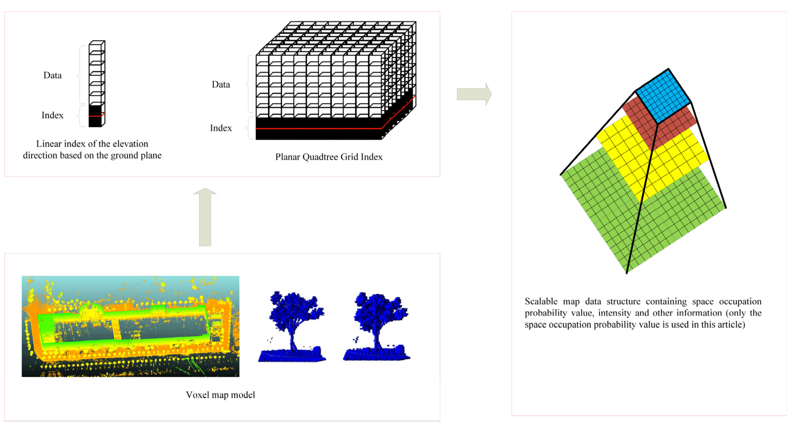
Figure 1. 3D EQT map model based on planar quadtree and elevation index.
Remotesensing 15 00595 g001
Figure 2. Scan-to-map matching algorithm.
Remotesensing 15 00595 g002
Figure 3. The MMS built in this paper integrates LiDAR, GNSS, IMU, and the Raspberry Pi operating system, which can be controlled by a mobile phone. (A) is a GNSS antenna; (B) is a VLP-16 LiDAR; (C) is internally integrated with the Raspberry Pi operating system, IMU, and GNSS board.
Remotesensing 15 00595 g003
Figure 4. Test environment of industrial park. (a) is point cloud maps of industrial park, the red line indicates the test route; (b) is the experimental site environments.
Remotesensing 15 00595 g004
Figure 5. Test environment of road environment. (a) is the point cloud maps of road environment, the red line indicates the test route; (b) is the experimental site environments.
Remotesensing 15 00595 g005
Figure 6. The number of available GNSS satellites and DOP value in the industrial park environment.
Remotesensing 15 00595 g006
Figure 7. The number of available GNSS satellites and DOP value in the road environment.
Remotesensing 15 00595 g007
Figure 8. Time series and boxplots of positioning errors in industrial parks. (a) is time series of positioning errors and (b) is boxplots of positioning errors.
Remotesensing 15 00595 g008
Figure 9. Time series and boxplots of positioning errors in road environments. (a) is time series of positioning errors and (b) is boxplots of positioning errors.
Remotesensing 15 00595 g009
Figure 10. (a) is a pre-built point cloud map; (b) is a picture of a real underground mine tunnel environment; (c) is the point cloud perspective of Faro.
Remotesensing 15 00595 g010
Figure 11. (a) Underground mine tunnel trajectory; (b) Underground mine tunnel trajectory from XYZ view; (c) Projection of the trajectory inside the red ellipse in (a) onto XY plane; (d) Projection of the trajectory inside the red box in (b) onto XY plane.
Remotesensing 15 00595 g011
Figure 12. (a) Difference between trajectory Traj_A and Traj_B; (b) Difference between trajectory Traj_A and Traj_C; (c) Difference between trajectory Traj_A and Traj_NDT.
Remotesensing 15 00595 g012
Figure 13. Positioning trajectories between ore loading and unloading points based on EQT map with resolution of 8 cm.
Remotesensing 15 00595 g013
Figure 14. APE result and trajectory of KITTI dataset 00.
Remotesensing 15 00595 g014
Figure 15. APE result and trajectory of KITTI dataset 10.
Remotesensing 15 00595 g015
Figure 16. Compute time cost of using the Bursa model and rotation matrix model; the compute time difference between them is the blue line.
Remotesensing 15 00595 g016
Figure 17. Positioning result difference of using the Bursa model and rotation matrix model.
Remotesensing 15 00595 g017
Table 1. Characteristics of the gyroscopes and accelerometers of the Honeywell HG4930 imu.
DeviceSensorIn Run Bias Variation at Constant TemperatureRandom WalkMax Input
Honeywell HG4930Gyroscope1°/h0.09°/√hr±200°/sec
Accelerometer0.3 mg30 ug/√Hz±20 g
Table 2. File size of different resolution industrial parks and roads on the EQT map, PCD file size.
ScenesResolutionMap File Size (KB)
Industrial park8 cm31,849
16 cm7033
24 cm3084
NDT(PCD file)535,314
Roads8 cm64,498
16 cm16,453
24 cm7820
NDT(PCD file)845,191
Table 3. The RMS of position error using different resolution maps in different scenes.
ScenesMap ResolutionPosition Error RMS(m)
NEDTotal
Industrial park8 cm0.0420.0420.0610.086
16 cm0.0590.0570.0660.105
24 cm0.0710.0730.0780.129
NDT0.2070.1720.1350.301
Roads8 cm0.0260.0260.0680.077
16 cm0.0250.0260.0780.076
24 cm0.0320.0300.0790.090
NDT0.0600.0760.1120.148
Table 4. The RMS of attitude error using different map resolution in different scenes.
ScenesMap ResolutionAttitude Error RMS (°)
RollPitchYaw
Industrial park8 cm0.0450.0560.162
16 cm0.0600.0920.163
24 cm0.1080.1380.146
NDT0.2150.4550.519
Roads8 cm0.1290.1410.132
16 cm0.1360.1450.138
24 cm0.1410.1490.130
NDT0.3740.3390.134
Table 5. Quantitative analysis: the percentage of positioning results better than 0.1 m, 0.2 m, 0.3 m, and max position error.
ScenesMap ResolutionPosition Error Percentage Statistics
<0.1 m<0.2 m<0.3 mMax
(m)
Industrial park8 cm85.98%98.88%99.94%0.321
16 cm67.76%97.41%99.49%0.404
24 cm42.00%93.40%99.39%1.072
NDT0.60%26.41%63.90%1.154
Roads8 cm78.70%99.63%100.00%0.229
16 cm80.94%99.00%99.90%0.257
24 cm80.90%95.84%99.58%1.039
NDT14.56%68.94%95.79%1.370
Table 6. Quantitative analysis: the percentage of attitude results better than 0.1°, 0.2°, 0.3°, and max attitude errors.
Map ResolutionAttitude Error Percentage Statistics
<0.1°<0.2°<0.3°Max (°)
Industrial park8 cmR91.52%99.58%100.00%0.284
P96.92%99.73%100.00%0.327
Y45.58%92.35%97.16%1.423
16 cmR77.92%95.92%98.91%0.554
P92.21%99.44%99.89%0.464
Y60.74%93.63%96.45%1.386
24 cmR59.11%87.15%97.31%1.372
P73.27%94.25%97.60%0.666
Y68.23%92.85%96.31%1.222
NDTR32.01%67.21%86.06%1.743
P28.70%46.43%59.34%2.67
Y31.62%57.92%78.72%1.933
Roads8 cmR60.39%90.73%97.44%0.508
P56.33%84.79%96.86%0.512
Y51.73%85.05%96.82%0.721
16 cmR59.72%89.22%96.11%0.600
P54.67%83.93%96.17%0.837
Y50.22%84.75%96.71%0.433
24 cmR59.85%87.30%94.60%0.560
P52.02%83.32%94.86%0.515
Y56.27%86.08%97.29%0.501
NDTR6.00%19.65%41.28%2.035
P15.21%34.00%56.06%2.438
Y63.28%89.11%93.86%1.708
Table 7. Average time cost of scan-to-map matching in industrial parks and roads.
ScenesMap ResolutionAverage Time Cost (ms)
Industrial park8 cm34.8
16 cm32.3
24 cm29.2
NDT37.1
Roads8 cm33.0
16 cm32.4
24 cm31.4
NDT45.9
Table 8. File sizes for different resolution the EQT map of mine tunnel, PCD file size.
ScenesMap ResolutionMap File Size (KB)
Mine Tunnel8 cm4364
16 cm1366
24 cm1038
NDT(PCD file)422,621
Table 9. Average time cost of scan-to-map matching in underground mine tunnel.
ScenesMap ResAverage Time Cost (ms)
Mine Tunnel8 cm18.7
16 cm19.9
24 cm19.8
NDT34.7
Table 10. APE results of KITTI dataset.
0001020304050607080910
Max (m)1.4050.1832.1460.1570.1310.5570.6080.2761.8330.1810.115
Mean (m)0.1460.0420.0450.0320.0270.0440.0330.0420.0560.0350.027
RMSE (m)0.3010.0500.0820.0400.0350.0650.0450.0550.1860.0420.033
STD (m)0.2630.0270.0690.0240.0220.0480.0300.0360.1770.0240.018
ATC (ms)39.337.139.741.237.341.737.938.037.238.339.7
Disclaimer/Publisher’s Note: The statements, opinions and data contained in all publications are solely those of the individual author(s) and contributor(s) and not of MDPI and/or the editor(s). MDPI and/or the editor(s) disclaim responsibility for any injury to people or property resulting from any ideas, methods, instructions or products referred to in the content.