Abstract
Picking the reflection horizon is an important step in velocity inversion and seismic interpretation. Manual picking is time-consuming and no longer suitable for current large-scale seismic data processing. Automatic algorithms using different seismic attributes such as instantaneous phase or dip attributes have been proposed. However, the computed attributes are usually inaccurate near discontinuities. The waveforms in the horizontal direction often change dramatically, which makes it difficult to track a horizon using the similarity of attributes. In this paper, we propose a novel method for automatic horizon picking using multiple seismic attributes and the Markov decision process (MDP). For the design of the MDP model, the decision time and state are defined as the horizontal and vertical spatial position on a seismic image, respectively. The reward function is defined in multi-dimensional feature attribute space. Multiple attributes can highlight different aspects of a seismic image and therefore overcome the limitations of the single-attribute MDP through the cross-constraint of multiple attributes. The optimal decision is made by searching the largest state value function in the reward function space. By considering cumulative reward, the lateral continuity of a seismic image can be effectively considered, and the impacts of abnormal waveform changes or bad traces in local areas for automatic horizon picking can be effectively avoided. An effective implementation scheme is designed for picking multiple reflection horizons. The proposed method has been successfully tested on both synthetic and field data.
1. Introduction
In exploration seismology, the reflection horizons in imaging volumes play an important role in velocity inversion and seismic interpretation. For velocity inversion, the reasonable application of the reflection horizon can effectively improve the convergence and obtain a geologically plausible velocity model. For seismic interpretation, the main reflection horizon can determine the relationship between geological layers and improve the reliability and accuracy of seismic interpretation. Therefore, automatically and efficiently picking the horizons from a complex seismic image is very important.
There are two main methods for tracking horizons. The first method is to identify and extract the horizon position using various signal or image processing methods based on various seismic attributes. For example, we can use the amplitude attribute [1], phase attribute [2,3,4,5,6], waveform attribute [7,8,9], and slope or dip attribute [10,11,12,13,14,15,16,17] to track the horizon. Furthermore, multiple attributes can be combined to constrain the picking results [18,19,20,21,22,23], such as using the instantaneous phase and dip attributes [18,22] and using the envelope, phase attributes, and texture analysis [23]. In addition, there are also various tracking algorithms for horizon picking. Admasu and Tönnie [24] used the correlation of horizons across faults in 3D seismic data, and Zou et al. [9] tracked the horizon based on the waveform similarity. Bondár [25] used the edge detection algorithm to detect seismic horizons. Aurnhammer and Tonnies [26] used a genetic algorithm for automated horizon correlation across faults in seismic images. Many global methods [27,28,29] or the flattening method [12,13,14,30,31,32,33,34] are also widely used for automated horizon picking.
The second method is mainly based on the Machine Learning (ML) algorithm to intelligently track the horizon; it mainly includes supervised learning methods with artificial neural networks [35,36,37,38,39], convolutional neural networks [40,41,42,43,44,45], and unsupervised learning methods with self-organizing networks [46] and convolutional auto-encoding networks [47].
In the first method, conventional horizon-picking methods depend heavily on the seismic attribute. When the attribute changes in the horizontal direction are relatively dramatic, it is difficult to track the correct horizon position. With the help of big data and ML methods, we can learn the structural information of the seismic image according to the data’s statistical characteristics. However, supervised learning methods need a lot of training data and labels, and the results obtained using unsupervised network algorithms are often unreliable.
If the problem of automatic horizon picking is regarded as an optimal decision-making process, a kind of ML method named reinforcement learning, the core algorithm of which is based on the Markov decision process (MDP), can be used to replace manual picking by imitating human behavior. The MDP based on the Markov chain can perceive the state change in the system environment and simulate humans to make a decision. Wald [48] adopted the MDP to solve the sequential analysis problem. Shapley [49] introduced a Markov decision process when studying random games. Bellman [50] put forward the discrete-time MDP (Bellman equation) for dynamic programming, which established a complete methodology of MDP. With the improvement of the MDP theory and method [51,52,53], the MDP method has been widely used in sequential decision making [54,55,56], dynamic programming [53,57], and reinforcement learning [58,59]. In the exploration seismology, Ma et al. [60] introduced reinforcement learning for selecting the first arrival. Luo et al. [61] designed a Markov decision process for first break picking.
In this paper, we formulate the horizon picking of seismic images as a Markov decision process (MDP) with multiple seismic attributes. The paper is organized as follows: Firstly, this paper briefly reviews the basic concepts and algorithms of the MDP. Then, the finite-stage MDP is designed for automatic horizon picking. For the MDP, the decision time is defined as the horizontal spatial position, and the state is defined as the vertical spatial position on the seismic image. The reward function is defined in multi-dimensional feature attribute space including the waveform attribute, instantaneous phase attribute, envelope attribute, and extremum attribute. When the seed point is determined, we can perceive the state change and take some actions to obtain reward value, where the selected action depends on the dip attribute. Therefore, we can make the optimal decision for horizon picking through constant trial and error and interaction with the environment. Moreover, for picking multiple reflection horizons, we design an effective implementation scheme using multiple seismic attributes and MDP. Finally, synthetic and field data are used to verify the effectiveness of the proposed method.
2. Review of the Markov Decision Process
2.1. 5-Tuple <>
The Markov decision process (MDP) mainly includes the following elements: state (), action (), policy (), transition probability (), and reward function ().
--State: The state is defined as one of the system characteristics at the decision-making time . If a state does not change with time, the state becomes , called a stable state. State space is defined as a finite set , where is the size of state space.
--Action: The action is the response of a system to the state . For a certain state , the set of all possible actions can be expressed as . The action space of a system is defined as the union composed of action sets under all states , where is the size of action space.
--Policy: The mapping process from state to action is called policy . The policy depends on the whole decision process, and the sequence formed by the mapping of state to action at all times is called a policy :
where is the probability of mapping state to action . The policy space is defined as a finite set , where is the size of the policy space.
--Transition probability: When performing an action from one state at the time , the system makes a transition to a new state , where the transition is based on a probability distribution . The transition probability of the system from the state to the state is:
According to Markov property, the state of a system at the time only depends on the state at the time and is independent of the previous state:
--Reward Function: The reward function is defined as ,
where is the reward function when the system executes action under the state at the time , then transfers to the state . The reward function is only related to the current state and action and has nothing to do with the previous state and action.
2.2. The Markov Decision Process
By integrating the above elements, we can define the MDP model, which can be viewed in Figure 1. This process can be completely described as: at the time , the system is in the state , and the decision-maker executes action and generates reward value and then transfers to the next state with probability function . The model forms the complete MDP time series at all times, which can be expressed as:

Figure 1.
The MDP model.
Taking a decision (with an action) according to policy from the state at the time , the system can obtain a reward sequence at the subsequent time,
where is the immediate reward function. The overall expectation from the immediate reward function to the future reward function sequence with the policy is defined as value function :
where is the expectation and is the discount factor, and , which means that the further the reward is from the decision-making time, the smaller the impact on the value function. Based on the Markov property, Formula (7) can be written as:
This equation is the so-called Bellman equation [50] or the state transition equation. Based on the Bellman equation, the state value function at the current time can be calculated by the state value function of the next decision time.
The value function is used to evaluate how “good” a decision-maker is in a given state [59]. The goal of the MDP model is to find the best policy that can maximize the value function. Therefore, an optimal policy is defined as for all and all policies . The optimal solution satisfies the following Bellman optimality equation:
Once the MDP model is determined, an appropriate and effective solution method can be selected to obtain the optimal policy, for example, the value iteration method [50], the policy iteration method [51], the Q learning algorithm [58], or the SARSA [62].
3. Formulation of Horizon Picking with MDP
For the problem of automatic horizon picking on seismic images, we can regard the seed point of one reflection horizon as the initial state and take some action policies to track the horizon. Based on the reward function of the current state (vertical position) and action, we can find an optimal policy to transfer to a new state at the next decision time (horizontal position). The state and transition probability distribution only depend on the current position and have nothing to do with the state and action of the previous position. Therefore, we regard the automatic horizon picking on the seismic image as an intelligent decision-making problem in a random environment which can be modeled as a discrete MDP with finite stages.
The horizon-picking model with finite-stage MDP is defined as follows:
(1) Decision time
The decision time is defined as the horizontal spatial position where the vertical and horizontal grid number is and , respectively, for a 2D seismic image.
According to the position of the seed point, the decision-making time can be divided into three categories:
(a) The starting time is at the left endpoint , and the ending time is at the right endpoint . The decision time sequence is .
(b) The starting time is at the right endpoint , and the ending time is at the left endpoint . The decision time sequence is .
(c) The starting time is at the middle position . The decision time is divided into two parts: one is to track to the right endpoint (consistent with mode a); the second is to track to the left endpoint (consistent with mode b).
(2) State
The state is defined as the vertical spatial position on a seismic image. The set of states is represented as . A seismic image often contains multiple horizons. When we pick one of them, the rest are irrelevant. The farther away an image is from the current axis in the vertical direction, the less influence it has on the decision. Moreover, we reduce the state space to , where is the width. is the middle position of the state space, which is determined by the conventional picking method. Particularly, is the seed point. The reduction in state space can not only weaken the impact of another horizon, but also improve computational efficiency.
(3) Action
The action is defined as a movement from a lateral position to a lateral position , .
(4) Policy
We adopt the stochastic policy to realize the mapping from state to action under the constraint of the dip attribute
where is the dip at the position of the state , and and are the sampling intervals in the lateral and vertical directions, respectively. is the variance in the Gaussian probability distribution. Figure 2 shows the mapping probability diagram from state to action. Following the dip direction, the probability of action is high. Staying away from the dip direction, the probability of action slowly becomes smaller. When the state position changes, the corresponding action probability density function also changes.
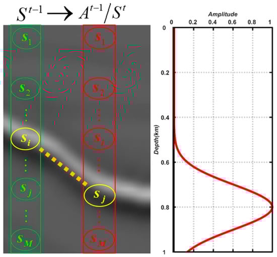
Figure 2.
The diagram of the mapping process of the state to action. The background profile in the left figure is a local seismic image. The right figure shows the probability distribution followed by the relationship between state and action where the position of the current state at the time is located at , and the state will move to next time . The yellow dashed line is the direction corresponding to the dip angle calculated at the position . The probability at is maximum. Away from , the probability is getting smaller.
(5) Transition probability
For state and action at time , the state at time is relatively independent. The transition probability is defined as
Therefore, the transition probability of the system from the state to the state is:
(6) Reward function
In the MDP, the optimal state is found according to the value function. However, the value function depends on the reward function. The reward function is the most important part of the MDP, which implicitly defines the learning objective [59]. In this paper, we use multiple seismic attributes of the seismic image to define the reward function.
Based on Formula (4) and (11), the relationship between the reward function and is as follows:
Therefore, the reward function is defined as
where is the distance between the state and for the attribute . The operator is a measure of attribute difference. is the maximum reward value, is the reward value, and is the weight coefficient of the attribute . The weighting coefficient is determined by the Fuzzy C-Means (FCM) clustering method, where the result is obtained by using the conventional horizon-picking method with a single attribute.
In this paper, the following attributes are selected to calculate the reward function:
(a) The waveform similarity for :
where is the size of the local space window, and is the similarity coefficient.
(b) The extremum attribute for :
where the attribute includes the waveform attribute, instantaneous phase attribute, and envelope attribute.
The instantaneous attributes of the seismic image can be obtained by applying a Hilbert transform to generate complex signals. For a 2-D seismic image , the is treated like a real part of the complex signals, and the imaginary part can be obtained after the Hilbert transformation. The complex signals are:
Then, the envelope and the instantaneous phase can be obtained by
However, the range of the instantaneous phase solved by Equation (20) has discontinuity. Based on the relationship between the seismic image and its transformation result:
The instantaneous phase can also be represented as
Furthermore, we use the least squares inverse division [63] to avoid the instability caused by zero division:
Finally, the instantaneous phase is calculated as
where is a threshold coefficient.
Then, we use the structure tensor method to calculate the dip attribute. Considering the waveform oscillation of seismic image, the structure tensor is obtained using the envelope attribute:
where represents the gradient of the envelope, and and are the directional derivatives in the direction and direction, respectively.
The eigenvalues and eigenvectors of the structure tensor matrix are obtained by eigenvalue decomposition of the structure tensor matrix:
where and are the eigenvalues, and and are the corresponding eigenvectors, respectively. represents the tensor energy of the first eigenvector, which is consistent with the direction of the gradient. The orientations of the eigenvector and are:
where is the gradient direction.
(7) Discount factor
Considering the impact on the subsequent limited-time steps, the discount factor is defined as
where is the maximum time step, and , is the current time. Figure 3 shows the discount factor for . As the time step gets further away, the discount factor gets smaller, and the subsequent value function becomes less influential on the decision.
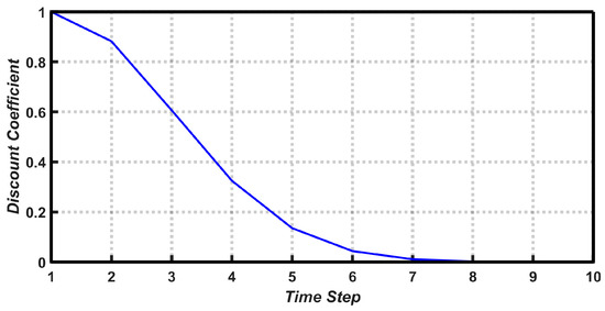
Figure 3.
The discount factor for the MDP model.
4. An Effective Scheme for Horizon Picking
We designed an effective implementation scheme for automatically picking multiple horizons using multiple seismic attributes and MDP, shown in Figure 4. The scheme mainly includes five parts as follows:
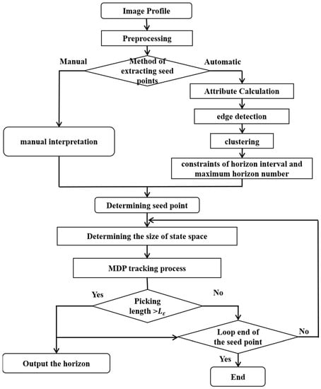
Figure 4.
The flowcharts for the horizon picking of the proposed method.
(1) Preprocessing the seismic image.
The seismic image contains not only multiple horizons but also various coherent and incoherent noises. The proper preprocessing method can highlight wavelet characteristics and suppress some noises. We use the structural smoothing filtering method to process the seismic image.
(2) Determining the position of the initial seed point
We proposed two methods to obtain the seed point to adapt the different applications. One method is to rely on manual interpretation, and the second method is to use edge detection and clustering to obtain seed points automatically. For the automated method, firstly, we use an edge detection method to calculate edge points with different seismic attributes, and then cluster these edge points together to obtain the corresponding center point location. Last, the initial seed points are determined by the constraints of horizon interval and maximum horizon number. The second method is mainly aimed at the process of automatically determining seed points, such as extracting structural information in inversion iteration. However, for complex imaging results, we prefer manual interpretation.
(3) Determining the size of state space
According to the position of seed points , we use the conventional method (waveform, phase, and extremum attributes) to pick up the horizon. Then, the location is determined by superimposing these conventional results to form the initial state.
where are the results of the waveform, phase, and extremum attributes, respectively.
(4) MDP tracking process
After defining the MDP model with multiple seismic attributes, the optimal state (horizon position) can be obtained by the state value function. When the following conditions are met during MDP, the tracking will stop:
(a) When the decision time reaches the end point (the boundary of the profile), it automatically turns to the termination state and records the length of the horizon.
(b) When the long-term value function is less than the given threshold (it means that this may encounter a fault), the system will turn to the termination state and record the length of the horizon.
(5) Output the tracking result
If the length of the horizon is less than the given threshold length, the horizon will be discarded, and the MDP tracking process will be started with the new seed point. On the contrary, we will output the horizon as the final result.
5. Numerical Examples
In this section, we illustrate the effectiveness of the proposed automatic horizon-picking method in both synthetic and field data examples.
5.1. A Local Layered Model
In the first example, we use the migration result of a synthetic model to demonstrate the validity of the proposed method. Figure 5a shows the local seismic image under the condition of inaccurate migration velocity. A large number of migration artifacts appear in the profile, and the waveforms change rapidly along the horizons. The attributes of the envelope, instantaneous phase, and dip are shown in Figure 5b–d. As can be seen, the different attributes can highlight the partial characteristics of the seismic image. For example, when the envelope attribute occurs discontinuously (as shown in the black box in Figure 5b), the phase attribute has good continuity (as shown in the black box in Figure 5c). Multiple attributes can be used to supplement each other’s defects. However, not all attributes may be good. At this time, if we take a conventional method such as single-trace-picking-based similarity, the reflection horizon cannot be traced accurately. Although all attributes are not good in local areas, they have certain similarities in the horizontal neighborhood of the area. This means that we can use the attributes of a neighborhood of the area to determine the horizon using a multi-step prediction method such as the MDP method. Figure 5e shows the results of the conventional single trace cross-correlation picking method and the proposed method using the multiple attributes with MDP. The sharp changes in the waveform in the horizontal direction and the attribute differences in the region lead to the inability of the conventional picking method to correctly pursue the horizon position. The Markov decision process method based on multi-attribute and multi-trace rewards can effectively avoid local noise interference and successfully track the correct reflection horizon.
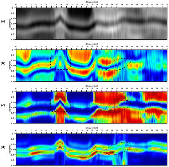

Figure 5.
(a) Local migration imaging results, (b) envelope, (c) instantaneous phase, (d) dip, and (e) tracked horizon (the blue curve is the result via conventional waveform similar method, and the red curve is the result via the proposed method) overlaid with seismic image.
5.2. The North Sea F3 Field Data
The second example illustrates the application of the proposed method to a real 3-D seismic survey F3 acquired over the North Sea. The extracted slice is shown in Figure 6a, and the instantaneous phase attribute is shown in Figure 6d. We observe that there is an obvious reflection horizon shown as the red arrow, and there is also a horizon with weak amplitude and less continuity, within the depth range of 0.8 km~0.9 km and the horizon position 0~1 km. Figure 6b,e show the troughs of the seismic data and the instantaneous phase attribute. Figure 6c,f show the peaks of the seismic data and the instantaneous phase attribute. Whatever a trough or a peak is shown the seismic data and the instantaneous phase attribute, the horizon shows poor continuity, which is marked by circles shown in Figure 6b,c,e,f. We cannot pick the correct reflection horizon according to any of these attributes. Figure 6g,h show the tracked horizon (red curve) using our proposed method on the image and waveform of seismic data, respectively. The blue cross symbols in Figure 6g,h are the seed points obtained via manual interpretation. Note that the waveform is similar and easy to track within the left portion and the right portion of the seismic slice. The waveform changes rapidly within the middle portion of the seismic slice, which makes it difficult to obtain the correct horizon position via the conventional method. However, the tracked horizon using the proposed method exactly follows the seismic reflection event.
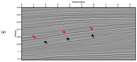
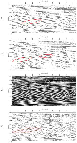

Figure 6.
The result for an extracted inline slice of F3 seismic data. (a) Seismic data, (b) troughs of seismic data, (c) peaks of seismic data, (d) instantaneous phase attribute, (e) troughs of instantaneous phase, (f) peaks of instantaneous phase, and tracked horizon (red curve) overlaid with (g) image and (h) waveform of seismic data.
5.3. The Overthrust Model for Picking Multiple Horizons
The third example illustrates the application to the overthrust model for picking multiple horizons. Figure 7a shows the migration imaging result with the background velocity model. In this example, we use the automated method to obtain seed points. The maximum number of seed points is set to eight, the minimum interval of the horizon is 0.1 km, and the minimum length is 1/10 of the number of lateral points. After the edge detection and clustering with the constraints of horizon interval and maximum horizon number, eight seed points are automatically obtained, which are marked by stars shown in Figure 7b. The tracked horizons with red curves using the proposed method overlaid on the seismic image are shown in Figure 7b. Because of the inaccurate migration velocity, the reflection horizon in the migration seismic image is not focused and discontinuous, shown as the black arrows, which makes it difficult to pick the correct reflection horizon information by using the conventional method. The reflection structure extracted using the proposed method is consistent with the real structure, which shows the effectiveness of this method. Therefore, the desired reflection horizons can be selected effectively and applied to the process of velocity modeling and the seismic interpretation process.
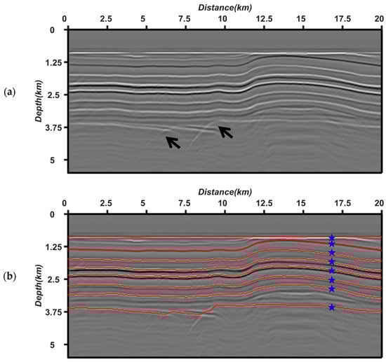
Figure 7.
The overthrust model result. (a) Seismic image and (b) tracked horizons (red curve) overlaid with the seismic image.
5.4. The Field Data for Picking Multiple Horizons
We further test the effectiveness of the proposed method by using the migration image from a field dataset acquired on land. The tracked horizons with red circles using the proposed method overlaid on the local migration image are shown in Figure 8. The horizons have a small interval, and multiple waveforms are stacked together. Therefore, we cannot extract the complete wavelet waveform. This is very common in sandstone thin interbed reservoirs and is exacerbated when the result is included in internal multiples. Given the seed points, we can trace the right horizons from the superimposed waveform. The position of the extracted horizons is consistent with the initial state positions.
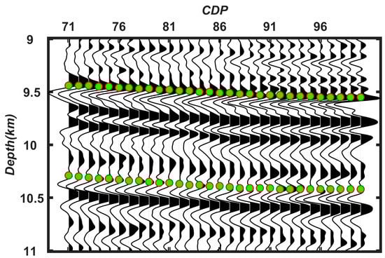
Figure 8.
The extracted horizons for land data.
Finally, we apply the proposed method to field offshore data. Figure 9a shows the migration imaging result in the background velocity model from the original observed seismic data. Figure 9b shows the tracked horizons with a red curve overlaid on the migration image. The blue stars in Figure 9b are the positions of the seed points obtained via manual interpretation. As can be seen, the picking result of the proposed method is still very good, even when dealing with an actual complex seismic image.
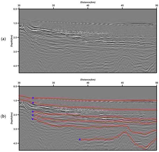
Figure 9.
The extracted horizons for real offshore data. (a) Seismic image and (b) tracked horizons (red curve) overlaid with the seismic image.
6. Discussion
An appropriate data preprocessing method can effectively improve the accuracy of horizon picking. A seismic image contains not only multiple horizons but also various coherent and incoherent noises. For example, due to inaccurate migration velocity, serious migration artifacts will interfere with the continuity of the waveform. The migration operator is not amplitude-preserving, resulting in a large amplitude difference in the transverse direction of horizons. Therefore, various methods (such as a amplitude-preserving migration algorithm, edge-preserving smoothing, and a denoising method) can be applied to improve the imaging quality. For the problem that the imaging result is not focused due to an inaccurate migration velocity model, we can extract the common-image gathers (CIGs), then the flattening and denoising operators can be applied to the CIGs, and the focused imaging result can be obtained by optimal stacking [64].
The imaging results cannot be directly mapped to horizons. It is necessary to extract some attributes of a seismic image and highlight the difference between the horizon and noise, so as to detect and extract the horizon. The purpose of attribute extraction is to highlight the feature information and eliminate redundant and irrelevant information in a seismic image. However, the waveform in the horizontal direction changes dramatically, and one single attribute often cannot trace to the correct horizon. Multiple attributes can highlight different aspects of seismic image properties. It is necessary to use multiple attributes to make up for the shortcomings of a single attribute. Therefore, the reward function is defined according to the similarity of multiple attributes for adjacent traces. The more attributes there are, the more information is available. However, it should be noted that the calculation of attributes must be accurate. Only correct attributes can contribute to picking. It is better to leave a deficiency uncovered than to have it covered without discretion. Attributes should be as independent as possible and highlight the structural features and similarities of the horizon.
Regarding horizon picking with the MDP, the key is to determine the state space, action space, and reward function. Considering the relationship between state and action at different times, and the similarity and continuity between the near horizons and inline or crossline slice, the association search constraint can be applied with the MDP. Through association search, we can transfer learning to the adjacent horizons or slices. Different MDP-solving methods can also be considered. Various kinds of reinforcement learning based on the MDP algorithm have been developed rapidly in recent years. For example, the Deep Q Network algorithm [65] can effectively search large-scale state space.
Moreover, when picking a horizon with faults, the MDP model needs to be optimized. The presence of a fault causes the low similarity of seismic attributes and low reward value. One solution is to place seed points on both sides of the fault. The position of the seed points will affect the picking result. The results are not the same for different positions of the seed points. The numbers and positions of seed points are also key factors. The method of obtaining seed points requires flexible selection through practical problems. The role of seed points is not only to provide the initial state but also to effectively select and extract the corresponding horizons.
In addition, for 2-D cases, we can regard the single horizon-picking problem as finding one optimal curve under the constraint of multiple seismic attributes. In the case of 3-D problems, the optimal curve will be replaced by the optimal surface. Tracing the optimal surface is a more complex problem. In this paper, we just explain how to track the horizon for a 2-D imaging section; extension to a 3-D problem with the MDP model is the next endeavor.
7. Conclusions
We propose a horizon-picking method based on multiple seismic attributes and the Markov decision process. We regard tracing reflection events on the seismic image as an intelligent decision problem. With the interaction process between the picking target and the environment, we can perceive the change of state and take some action to obtain reward value, where the reward function is defined by multiple seismic attributes. Multiple attributes can highlight different aspects of a seismic image and can make up for the shortcomings of a single attribute through the cross-constraint of multiple attributes. Then, the reward function will affect the state of the environment. Therefore, we can obtain the optimal picking horizon via the MDP model. Numerical examples on both synthetic and field data show that, by considering the optimal MDP with multiple attributes, we can avoid the influence caused by waveform changes in a single trace or a local area and pick up the desired reflection horizon robustly. The result of horizon picking can be used not only in velocity modeling but also in seismic interpretation.
Author Contributions
Conceptualization, C.W. and H.W.; methodology, C.W., B.F. and H.W.; writing—original draft and formal analysis, C.W. and X.S.; writing—review and editing, B.F., X.S., R.X. and S.S. All authors have read and agreed to the published version of the manuscript.
Funding
This research was funded by the National Natural Science Foundation of China ‘Research on Tomographic Inversion and Modeling Method of Characteristic Reflection Wave Theory’ (Grant No. 42174135), ‘Wave Equation Linearization and Velocity Inversion in Strong Scattering Media’ (Grant No. 42074143), the National Key R & D Program of China on Key Scientific Issues of Transformative Technologies ‘Multi-source information based joint seismic inversion’ (Grant No. 2018YFA0702503), and the SINOPEC Key Laboratory of Geophysics (33550006-20-ZC0699-0011; 33550006-22-FW0399-0019).
Data Availability Statement
Not applicable.
Acknowledgments
The author would like to thank China Petroleum Exploration and Development Research Institute and Northwest Branch, Sinopec Geophysical Exploration Technology Research Institute and Shengli Oilfield Branch, CNOOC Research Institute and Zhanjiang Branch for their funding and support for the research work of Wave Phenomenon and Intelligent Inversion Imaging Research Group (WPI).
Conflicts of Interest
The authors declare that they have no competing interest.
References
- Howard, R.E. Method for Attribute Tracking in Seismic Data. U.S. Patent No. 5,1991,056-066, 8 October 1991. [Google Scholar]
- Zeng, H.; Backus, M.M.; Barrow, K.T.; Tyler, N. Stratal slicing—Part 1: Realistic 3D seismic model. Geophysics 1998, 63, 502–513. [Google Scholar] [CrossRef]
- Stark, T.J. Unwrapping instantaneous phase to generate a relative geologic time volume. In 73rd Annual International Meeting, SEG, Expanded Abstracts; Society of Exploration Geophysicists: Tulsa, OK, USA, 2003; pp. 1707–1710. [Google Scholar] [CrossRef]
- Wu, X.; Zhong, G. Generating a relative geologic time volume by 3D graph-cut phase unwrapping method with horizon and unconformity constraints. Geophysics 2012, 77, O21–O34. [Google Scholar] [CrossRef]
- Dossi, M.; Forte, E.; Pipan, M. Automated reflection picking and polarity assessment through attribute analysis: Theory and application to synthetic and real ground-penetrating radar data. Geophysics 2015, 80, H23–H35. [Google Scholar] [CrossRef]
- Forte, E.; Dossi, M.; Pipan, M.; Ben, A.D. Automated phase attribute-based picking applied to reflection seismic. Geophysics 2016, 81, V141–V150. [Google Scholar] [CrossRef]
- Marfurt, K.; Kirlin, R.; Farmer, S.; Bahorich, M. 3-D seismic attributes using a semblance-based coherency algorithm. Geophysics 1998, 63, 1150–1165. [Google Scholar] [CrossRef]
- Lacaze, F.; Valding, T. Autopicking Velocity by Path-Integral Optimization and Surface Fairing. In 79th Annual International Meeting, SEG Expanded Abstracts; Society of Exploration Geophysicists: Tulsa, OK, USA, 2009; pp. 2592–2596. [Google Scholar] [CrossRef]
- Zou, G.; Ji, R.; Liu, W.; Zhang, J. Horizon auto-tracking technology based on the waveform similarity for the coalmining area seismic data. In Proceedings of the 2013 2nd International Symposium on Instrumentation and Measurement, Sensor Network and Automation (IMSNA), Toronto, ON, Canada, 23–24 December 2013; pp. 236–242. [Google Scholar]
- Gersztenkorn, A.; Marfurt, K.J. Eigenstructure-based coherence computations as an aid to 3-D structural and stratigraphic mapping. Geophysics 1999, 64, 1468–1479. [Google Scholar] [CrossRef]
- Bakker, P. Image Structure Analysis for Seismic Interpretation. Ph.D. Thesis, Delft University of Technology, Delft, The Netherlands, 2002. [Google Scholar]
- Lomask, J.; Guitton, A.; Fomel, S.; Claerbout, J.; Valenciano, A.A. Flattening without picking. Geophysics 2006, 71, P13–P20. [Google Scholar] [CrossRef]
- Lomask, J.; Guitton, A. Volumetric flattening: An interpretation tool. Lead. Edge 2007, 26, 888–897. [Google Scholar] [CrossRef]
- Parks, D. Seismic Image Flattening as a Linear Inverse Problem. Master’s Thesis, Colorado School of Mines, Golden, CO, USA, 2010. [Google Scholar]
- Wu, X. Directional structure-tensor-based coherence to detect seismic faults and channels. Geophysics 2017, 82, A13–A17. [Google Scholar] [CrossRef]
- Wu, X.; Fomel, S. Least-squares horizons with local slopes and multigrid correlations. Geophysics 2018, 83, IM29–IM40. [Google Scholar] [CrossRef]
- Di, H.; Gao, D.; AlRegib, G. 3D dip vector-guided auto-tracking for weak seismic reflections: A new tool for shale reservoir visualization and interpretation. Interpretation 2018, 6, SN47–SN56. [Google Scholar] [CrossRef]
- Lou, Y.; Zhang, B. Automatic horizon picking using multiple seismic attributes. In 88th Annual International Meeting, SEG Expanded Abstracts; Society of Exploration Geophysicists: Tulsa, OK, USA, 2018; pp. 1683–1688. [Google Scholar]
- Gogia, R.; Singh, R.; de Groot, P.; Gupta, H.; Srirangarajan, S.; Phirani, J.; Ranu, S. Tracking 3D seismic horizons with a new hybrid tracking algorithm. Interpretation 2020, 8, SQ39–SQ45. [Google Scholar] [CrossRef]
- Li, S.; Zhao, J.; Zhang, H.; Bi, Z.; Qu, S. A Novel Horizon Picking Method on Sub-Bottom Profiler Sonar Images. Remote Sens. 2020, 12, 3322. [Google Scholar] [CrossRef]
- Lou, Y.; Zhang, B.; Lin, T.; Cao, D. Seismic horizon picking by integrating reflector dip and instantaneous phase attributes. Geophysics 2020, 85, O37–O45. [Google Scholar] [CrossRef]
- Zhang, B.; Qi, J.; Lou, Y.; Fang, H.; Cao, D. Generating seismic horizon using multiple seismic attributes. IEEE Geosci. Remote Sens. Lett. 2020, 18, 979–983. [Google Scholar] [CrossRef]
- Zhao, J.; Li, S.; Zhao, X.; Feng, J. A Comprehensive Horizon-Picking Method on Subbottom Profiles by Combining Envelope, Phase Attributes, and Texture Analysis. Earth Space Sci. 2020, 7, e2019EA000680. [Google Scholar] [CrossRef]
- Admasu, F.; Tönnies, K.D. Model-based Approach to Automatic 3D Seismic Horizon Correlation across Faults. In Proceedings of the Simulation und Visualisierung 2004 (SimVis), Magdeburg, Germany, 4–5 March 2004; pp. 239–250. [Google Scholar]
- Bondár, I. Seismic horizon detection using image processing algorithms. Geophys. Prospect. 1992, 40, 785–800. [Google Scholar] [CrossRef]
- Aurnhammer, M.; Tonnies, K.D. A genetic algorithm for automated horizon correlation across faults in seismic images. IEEE Trans. Evol. Comput. 2005, 9, 201–210. [Google Scholar] [CrossRef]
- Pauget, F.; Lacaze, S.; Valding, T. A global approach in seismic interpretation based on cost function minimization. In 79th Annual International Meeting, SEG Expanded Abstracts; Society of Exploration Geophysicists: Tulsa, OK, USA, 2009; pp. 2592–2596. [Google Scholar]
- Hoyes, J.; Cheret, T. A review of global interpretation methods for automated 3D horizon picking. Lead. Edge 2011, 30, 38–47. [Google Scholar] [CrossRef]
- Hong, Z.; Su, M.; Qian, F.; Han, Q. Global seismic horizon interpretation based on data mining—A new tool for seismic geomorphologic study. Interpretation 2020, 8, T131–T140. [Google Scholar] [CrossRef]
- Wu, X.; Hale, D. Automatically interpreting all faults, unconformities, and horizons from 3D seismic images. Interpretation 2016, 4, T227–T237. [Google Scholar] [CrossRef]
- Jin, S.; Chen, S.; Wei, J.; Li, X. Automatic seismic event tracking using a dynamic time warping algorithm. J. Geophys. Eng. 2017, 14, 1138–1149. [Google Scholar] [CrossRef]
- Bugge, A.J.; Erik, L.J.; Evensen, A.K.; Faleide, J.I.; Clark, S. Automatic extraction of dislocated horizons from 3D seismic data using nonlocal trace matching. Geophysics 2019, 84, IM77–IM86. [Google Scholar] [CrossRef]
- Lou, Y.; Zhang, B.; Fang, H.; Cao, D.; Wang, K.; Huo, Z. Simulating the procedure of manual seismic horizon picking. Geophysics 2021, 86, O1–O12. [Google Scholar] [CrossRef]
- Yan, S.; Wu, X. Seismic horizon extraction with dynamic programming. Geophysics 2021, 86, 51–62. [Google Scholar] [CrossRef]
- Harrigan, E.; Kroh, J.R.; Sandham, W.A.; Durrani, T.S. Seismic horizon picking using an artificial neural network. In Proceedings of the IEEE International Conference on Acoustics, Speech, and Signal Processing, San Francisco, CA, USA, 23–26 March 1992; pp. 105–108. [Google Scholar]
- Huang, K. Hopfield neural network for seismic horizon picking. In 75th Annual International Meeting, SEG, Expanded Abstracts; Society of Exploration Geophysicists: Tulsa, OK, USA, 1997; pp. 562–565. [Google Scholar] [CrossRef]
- Huang, K. Neural network for seismic horizon picking. In IEEE International Joint Conference on Neural Networks Proceedings; IEEE World Congress on Computational Intelligence: Anchorage, AK, USA, 1998; Volume 3, pp. 1840–1844. [Google Scholar]
- Leggett, M.; Sandham, W.A.; Durrani, T.S. Automated 3-D Horizon Tracking and Seismic Classification Using Artificial Neural Networks; Springer: Cham, The Netherlands, 2003; pp. 31–44. [Google Scholar]
- Peters, B.; Granek, J.; Haber, E. Multi-resolution neural networks for tracking seismic horizons from few training images. Interpretation 2019, 7, SE201–SE213. [Google Scholar] [CrossRef]
- Waldeland, A.U.; Jensen, A.C.; Gelius, L.-J.; Solberg, A.H.S. Convolutional neural networks for automated seismic interpretation. Lead. Edge 2018, 37, 529–537. [Google Scholar] [CrossRef]
- Shi, Y.; Wu, X.; Fomel, S. SaltSeg: Automatic 3D salt segmentation using a deep convolutional neural network. Interpretation 2019, 7, SE113–SE122. [Google Scholar] [CrossRef]
- Wu, H.; Zhang, B.; Lin, T.; Cao, D.; Lou, Y. Semiautomated seismic horizon interpretation using the encoder-decoder convolutional neural network. Geophysics 2019, 84, B403–B417. [Google Scholar] [CrossRef]
- Yang, L.; Sun, Z. Seismic horizon tracking using a deep convolutional neural network. J. Pet. Sci. Eng. 2020, 187, 106709. [Google Scholar] [CrossRef]
- Tschannen, V.; Delescluse, M.; Ettrich, N.; Keuper, J. Extracting horizon surfaces from 3D seismic data using deep learning. Geophysics 2020, 85, N17–N26. [Google Scholar] [CrossRef]
- Zhang, K.; Lin, N.; Zhang, D.; Zhang, J.; Yang, J.; Tian, G. Automatic tracking for seismic horizons using convolution feature analysis and optimization algorithm. J. Pet. Sci. Eng. 2021, 208, 109441. [Google Scholar] [CrossRef]
- Huang, K.; Chang, W.; Lin, C. Self-organizing neural network for picking seismic horizons. In 60th Annual International Meeting, SEG Expanded Abstracts; Society of Exploration Geophysicists: Tulsa, OK, USA, 1990; pp. 313–316. [Google Scholar]
- Shi, Y.; Wu, X.; Fomel, S. Waveform embedding: Automatic horizon picking with unsupervised deep learning. Geophysics 2020, 85, WA67–WA76. [Google Scholar] [CrossRef]
- Wald, A. Foundations of a general theory of sequential decision functions. Econometrica. J. Econom. Soc. 1947, 15, 279–313. [Google Scholar] [CrossRef]
- Shapley, L.S. Stochastic games. Proc. Natl. Acad. Sci. USA 1953, 39, 1095–1100. [Google Scholar] [CrossRef]
- Bellman, R.A. Markovian decision process. J. Math. Mech. 1957, 6, 679–684. [Google Scholar] [CrossRef]
- Howard, R.A. Dynamic Programming and Markov Processes; John Wiley: Hoboken, NJ, USA, 1960. [Google Scholar]
- Blackwell, D. Discrete dynamic programming. Ann. Math. Stat. 1962, 33, 719–726. [Google Scholar] [CrossRef]
- Puterman, M.L. Markov Decision Processes: Discrete Stochastic Dynamic Programming; John Wiley & Sons: Hoboken, NJ, USA, 2014. [Google Scholar]
- Barto, A.G.; Sutton, R.S.; Watkins, C. Learning and Sequential Decision Making; University of Massachusetts: Amherst, MA, USA, 1989. [Google Scholar]
- Littman, M.L. Algorithms for Sequential Decision-Making; Brown University: Rhode Island, RI, USA, 1996. [Google Scholar]
- Read, P.; Lermit, J. Bio-energy with carbon storage (BECS): A sequential decision approach to the threat of abrupt climate change. Energy 2005, 30, 2654–2671. [Google Scholar] [CrossRef]
- Bertsekas, D. Dynamic Programming and Optimal Control: Volume I; Athena Scientific: Belmont, MA, USA, 2012. [Google Scholar]
- Watkins, C.J.C.H.; Dayan, P. Q-learning. Mach. Learn. 1992, 8, 279–292. [Google Scholar] [CrossRef]
- Sutton, R.S.; Barto, A.G. Reinforcement Learning; MIT Press: Cambridge, MA, USA, 1998. [Google Scholar]
- Ma, Y.; Fei, T.; Luo, Y. A new insight into automatic first-arrival picking based on reinforcement learning. In 81st EAGE Conference and Exhibition, Expanded Abstracts; European Association of Geoscientists and Engineers: Houten, The Netherlands, 2019; pp. 1–5. [Google Scholar]
- Luo, F.; Feng, B.; Wang, H. Automatic first-arrival picking method via intelligent Markov optimal decision processes. J. Geophys. Eng. 2021, 18, 406–417. [Google Scholar] [CrossRef]
- Sutton, R.S. Generalization in reinforcement learning: Successful examples using sparse coarse coding. In Advances in Neural Information Processing Systems; MIT Press: Denver, CO, USA, 1996; pp. 1038–1044. [Google Scholar]
- Wu, C.; Wang, H.; Feng, B.; Sheng, S. RTM angle gathers based on the Combining Local and Global (CLG) optical flow method and wavefield decomposition method. Chin. J. Geophys. 2021, 64, 1375–1388. (In Chinese) [Google Scholar] [CrossRef]
- Wu, C.; Wang, T.; Wang, H.; Luo, F.; Xu, P. Improving the quality of Common-Image Gathers using DTW and Local Similarity. In 89th SEG Annual International Meeting, Expanded Abstracts; Society of Exploration Geophysicists: Tulsa, OK, USA, 2019; pp. 4336–4340. [Google Scholar]
- Mnih, V.; Kavukcuoglu, K.; Silver, D.; Rusu, A.A.; Veness, J.; Bellemare, M.G.; Graves, A.; Riedmiller, M.; Fidjeland, A.K.; Ostrovski, G.; et al. Human-level control through deep reinforcement learning. Nature 2015, 518, 529–533. [Google Scholar] [CrossRef] [PubMed]


Disclaimer/Publisher’s Note: The statements, opinions and data contained in all publications are solely those of the individual author(s) and contributor(s) and not of MDPI and/or the editor(s). MDPI and/or the editor(s) disclaim responsibility for any injury to people or property resulting from any ideas, methods, instructions or products referred to in the content. |
© 2023 by the authors. Licensee MDPI, Basel, Switzerland. This article is an open access article distributed under the terms and conditions of the Creative Commons Attribution (CC BY) license (https://creativecommons.org/licenses/by/4.0/).