Article

Adaptive Feature Map-Guided Well-Log Interpolation

1
College of Science, China University of Petroleum, Changping, Beijing 102249, China
2
College of Geophysics, China University of Petroleum, Changping, Beijing 102249, China
*
Author to whom correspondence should be addressed.
Remote Sens. 2023, 15(2), 459; https://doi.org/10.3390/rs15020459
Submission received: 6 December 2022 / Revised: 9 January 2023 / Accepted: 9 January 2023 / Published: 12 January 2023
(This article belongs to the Special Issue Geophysical Data Processing in Remote Sensing Imagery)

Abstract

:
As an irreplaceable quantitative interpretation method, prestack seismic inversion enables the effective estimation of subsurface elastic parameters for reservoir prediction. However, for the model-driven prestack seismic inversion, the band-limited characteristics and noise interference of observed seismic data result in its high dependence on the initial models. This suggests that reasonable initial models act as a supplement to reliable variation trends in formation and can reduce the non-uniqueness of inversion results. In this article, we introduce a well-log interpolation method with a feature map-guided non-local means algorithm, which is for establishing high-fidelity initial models used for prestack seismic inversion. First, we briefly review the basic theory of general model-driven prestack seismic inversion. Then, we use dictionary learning to split the poststack seismic record into patches, and represent them with sparse vectors, instead of directly using seismic record. The advantage of dictionary learning is that it can adaptively extract useful signals from noisy observed data and provide fine structures by sparse reconstruction. Therefore, the proposed feature extraction method can improve the noise immunity and reliability of the well-log interpolation. More accurate initial models are pre-constructed efficiently by our feature extraction method, which improves the reliability of prestack seismic inversion results. Two kinds of observed seismic data are used, including the poststack seismic record for well-log interpolation and prestack seismic data used for inversion. Synthetic and field data tests both demonstrate the favorable performance of the proposed well-log interpolation method. In summary, a novel and convenient initial model building approach is provided, which contributes to seismic exploration and geologic modeling.

1. Introduction

Seismic inversion can interpret subsurface elastic parameters from observed seismic data; these include acoustic impedance, P-wave velocity (vp), S-wave velocity (vs), and density (ρ) [1,2,3,4,5]. The obtained subsurface elastic parameters are beneficial for reservoir prediction [6,7,8]. Poststack seismic data are self-simulation and self-received. Prestack seismic data reflect seismic amplitude variation with different incident angles. Compared with poststack seismic inversion, prestack inversion takes advantage of seismic amplitude versus offset (AVO) information, which can provide a wider range of elastic parameters for seismic interpretation.
The seismic amplitude can only depict the interface information of the horizons, e.g., the relative variation of elastic parameters [9]. Revealing subsurface quantitative elastic parameters is outside of the ability of seismic inversion relied on amplitude only. Initial models offer beginner value for seismic inversion, which is updated until the synthetic seismic data matches with observed data. The low-frequency initial model can reveal the variation trend of formation and provide an initial value for seismic inversion. However, if an initial model is deviated from the true situation, it will provide a biased inversion result, which leads to wrong interpretation results [10].
There are various initial model building methods, which can be divided into four categories [11,12,13,14]. First, velocity analysis picks the maximum energy of velocity spectra and interpolates the picked velocity points to obtain a low-frequency velocity model [15,16,17]. However, this method is dependent on the quality of seismic data and the accuracy of manual pickup. If the observed seismic record is of low quality, the energy of velocity spectra is unfocused, which makes it hard to determine the energy peaks. Second, travel time tomography takes into account that travel time is sensitive to low-frequency velocity, and utilizes travel time information to build an initial model [18,19,20]. It provides a velocity model by minimizing the misfit between the observed and forward modeling first arrivals. Generally, the travel time information for a given model is obtained by solving the eikonal equation. However, the tomography depends on the first break picking of the observed data. Third, the full-waveform inversion method uses the kinematic and dynamic information of the prestack seismic waves to recover the subsurface velocity structures [21,22,23]. However, its high computational cost, ill-posedness, and nonconvex nature of objective function limit its application and popularization. Fourth, the interpolation method guides the interpolation of filtered borehole curves depending on interpreted horizons. However, it requires a high amount of human intervention, which can easily introduce manual errors [24]. Moreover, horizon information is always limited, and geological details are hard to recover.
Recently, there has been increasing attention paid to seismic attributes-guided well-log interpolation [25,26,27,28,29], such as structure tensors [30,31], seismic slope [32], and prespecified filters [33]. Seismic attributes-guided well-log interpolation schemes can take advantage of seismic information rather than a few interpreted horizons with human intervention reduced. However, the interpolation results are sensitive to the reliability and accuracy of the extracted seismic attributes. Real seismic data are generally noisy and band-limited, so it is difficult to extract useful information based on manual specified attributes. The band-limited nature leads to smoother interpolated results when interpolated points are far away from wells. Additionally, the noise presented in observed data makes interpolation results biased from the true situation. In this paper, we utilize dictionary learning to sparsely code seismic sampling points, e.g., each seismic sampling point can be represented by a sparse vector under an adaptively learned dictionary. The successful application of dictionary learning in seismic processing indicates that these sparse vectors can efficiently represent useful information from the observed low-quality seismic record, and reduce the interference of band-limited nature and noise of seismic data as much as possible [34,35,36,37,38,39,40]. We apply the extracted feature maps in the non-local means algorithm (NLM) for well-log interpolation, which utilizes the similarity of feature maps to interpolate vp, vs, and ρ models between wells. Finally, we show the interpolated results for model-driven prestack seismic inversion to illustrate the proposed method’s performance.
The rest of this paper is organized as follows. First, we review the theory of general model-driven seismic inversion. Then, we introduce well-log interpolation by NLM, which utilizes the local seismic amplitude information. Additionally, we present the feature maps that are extracted from observed poststack seismic data based on dictionary learning. After that, to demonstrate the effectiveness of the proposed method, we apply the proposed interpolated methods on both synthetic and field data tests in view of interpolated results and model-driven prestack seismic inversion results.

2. Theory and Methods

2.1. General Model-Driven Prestack Seismic Inversion

Zoeppritz’s equation can describe the AVO phenomenon. However, it is a nonlinear equation for forward modeling and inversion [41]. In this paper, we conduct the prestack seismic inversion using one of its approximations, i.e., the Aki–Richards equation [42].
R ( θ ) 1 2 ( 1 4 v s 2 v p 2 sin 2 θ ) Δ ρ ρ + sec 2 θ 2 Δ v p v p 4 v s 2 v p 2 sin 2 θ Δ v s v s ,
where R(θ) represents the reflectivity at θ incident angle, vp, vs, and ρ represent P-wave velocity, S-wave velocity, and density, respectively, and Δvp, Δvs, and Δρ represent the difference of P-wave velocity, S-wave velocity, and density across an interface.
Based on the seismic convolution model, the prestack seismic data can be expressed by convolving seismic wavelets and reflectivities at different incident angles [43]:
d ( θ i a ) = W ( θ i a ) R ( θ i a ) , i a = 1 , 2 , , n a ,
where d(θia) denotes prestack seismic angle gathers, W(θia) represents the source wavelet corresponding to angle θia, denotes convolution operation, and na is the number of angle gathers. We assume that the wavelet is known, which can be obtained via wavelet extraction based on seismic data and well-log information or perhaps alternatively via the statistical methodology. Equation (2) can be represented in matrix form [44]:
d = WHm ,
where H denotes the product of coefficient matrix of (1) and the first-order difference matrix, m, represents the three parameters of vp, vs, and ρ to be inverted:
m = [ v p T v s T ρ T ] T .
The objective function for conventional model-driven prestack seismic inversion is constructed by seismic mismatch term and model constraint [45], which can be written as
min m d W H m 2 2 + λ m m 0 2 2 ,
where m0 represents the initial model by concatenating three elastic parameters, and λ is the regularization parameter controlling the contribution of the observed seismic data and the initial model to inversion results. The regularization term expects the inversion results approach to the initial model. In both synthetic and field data tests, we set λ based on the interpolated results compared with known borehole data. The initial model m0 is obtained by feature map-guided well-log interpolation, which will be illustrated in the following parts.

2.2. Well-Log Interpolation by Non-Local Means Algorithm

There are many studies indicating that the seismic-guided well-log interpolation can reduce manual interpretation errors, and adaptively interpolate borehole data along local seismic similarity or structure dip angles. However, these methods are usually time-consuming due to the inverse operation of the matrix.
To accelerate the interpolation’s computational efficiency, we utilize a non-local means (NLM) algorithm [46,47,48]. The surrounding Q known nodes are made with a weighted summation to calculate the value of one unknown node, which is expressed as
x i , j = q = 1 Q b i , j , q x i , j , q ,
where xi,j is the parameter at an objective point (i, j), j stands for the CDP number and i for the sampling point, xi,j,q is the number q well-log point to interpolate xi,j, and bi,j,q represents the weight coefficient, and Q stands for the number of samples of well log. To intuitively illustrate this workflow, we plot Figure 1 to show the schematic diagram for NLM, where CDP (common depth point) denotes the spatial location, and the time label represents the time duration of recorded data, which can reflect subsurface information at different depths. There are five reference points, e.g., Q = 5. The elastic parameter at one point is interpolated by weighted sum of five known reference points’ data, and the weight coefficients are calculated based on the similarity between seismic patches centered at the known reference and interpolated points. In each yellow box, the signals are weighted sum to get signal in green box. The weighted coefficients bi,j,q are used for interpolation in NLM algorithm. Based on the local seismic patches, the weight bi,j,q is given by
b i , j , q = 1 η exp ( R i , j s R i , j , q s 2 2 / h ) ,
where h is a prespecified hyper-parameter, Ri,j is an operator to extract the local seismic patch for which central point is located at number j CDP and number i sampling point, Ri,j,q is used to extract number q reference seismic patch, s denotes observed poststack seismic record, and η is defined as
η = q = 1 Q exp ( R i , j s R i , j , q s 2 2 / h ) ,
to ensure
q = 1 Q b i , j , q = 1 .
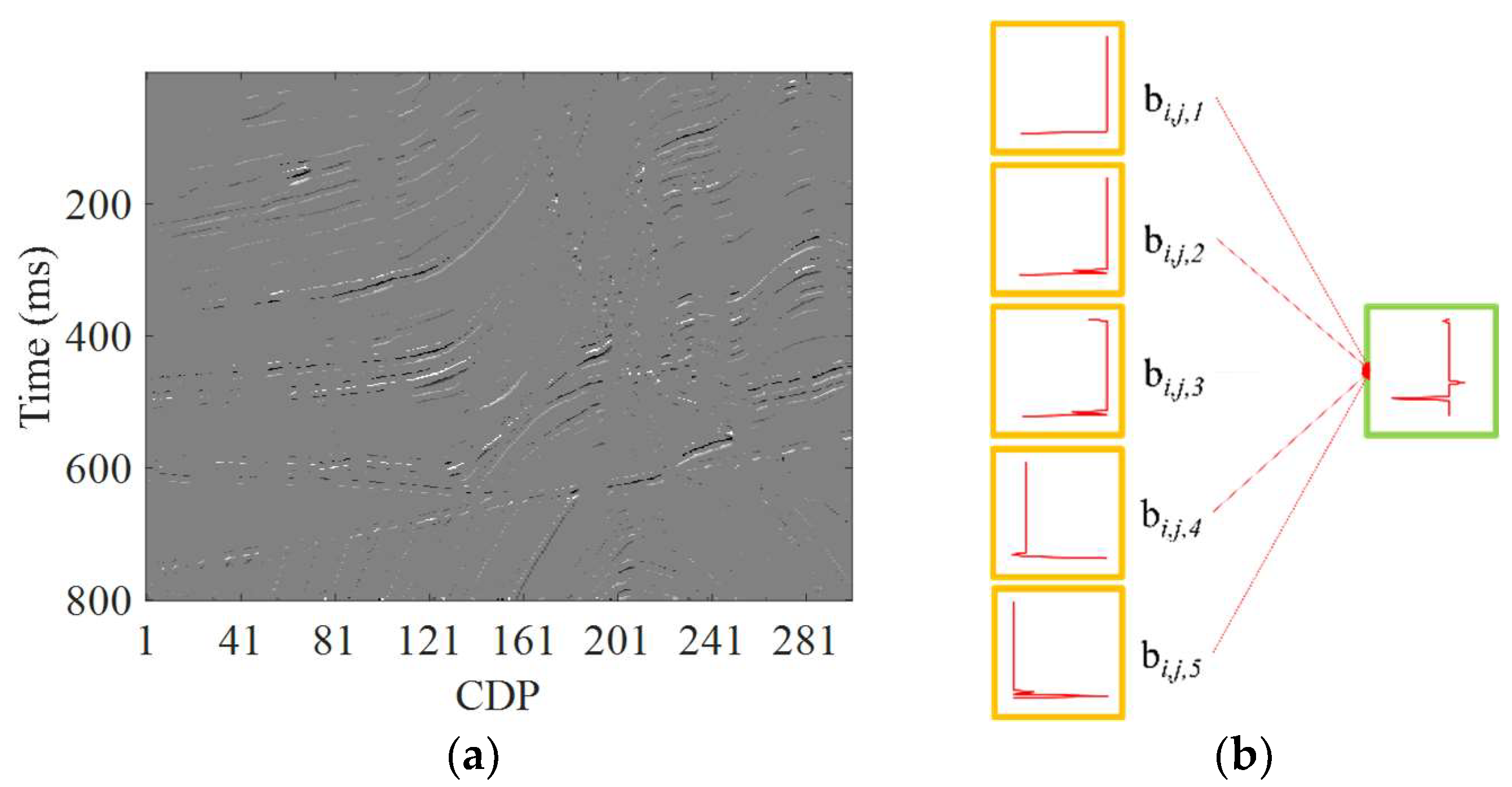
Seismic patches are extracted with a sliding window shown in Figure 2a. The red and yellow rectangles indicate the sliding window. The seismic profile is decomposed with the sliding window along vertical and horizontal directions. Each patch represents the local feature of the central sampling point. Therefore, we only show parts of seismic patches in Figure 2b.
Intrinsically, the well-log interpolation by NLM can be seen as the weighted summation of data at known nodes, and the weighting coefficients are calculated based on the local seismic similarity. However, the local seismic data may not reflect the accurate local subsurface structure features due to the noise interference and band-limited characteristics of seismic data. Although there are many attribute-guided approaches using multi-attribute regression to build a low-frequency model, it is also hard to select suitable attributes and extract useful signals due to the noise interference and bandlimited nature. The bandlimited nature always shows that one seismic event cannot describe a strata edge, which is an integrated response of multi-layers. Therefore, seismic data cannot directly reflect fine structures.

2.3. Feature Map Extraction from Observed Seismic Data

Accurate and antinoise features extracted from observed seismic data are beneficial to well-log interpolation, which can be used to determine the interpolation weight coefficients. Traditional interpolation methods only use the amplitude of observed seismic data or filtered seismic data by some prespecified filters. Here, we utilize dictionary learning to extract feature maps, and calculate the interpolation coefficients by replacing seismic patches in Equations (7) and (8) with sparse coefficients [49].
In the process of dictionary learning, the original seismic data are divided into seismic patches with a sliding window. This process is the same as Figure 2a. Each seismic patch is represented with the elastic parameter at the central sampling point. In dictionary learning, it is necessary to provide enough training samples, and seismic patch can effectively reduce computational cost. All seismic patches are used to train the dictionary and represented as sparse coefficients [50,51]. Each seismic patch Ri,js can be expressed as a linear combination of sparse coefficients αi,j and dictionary D, which are obtained by solving
min D , α i , j R i , j s D α i , j 2 2 s . t . α i , j 0 < T 0 ,
where         0 represents the l0 norm, which counts the number of nonzero elements, and T0 is the prespecified number of non-zero elements. In this paper, we update the dictionary by K-SVD (K-means singular value decomposition) algorithm and reconstruct sparse coefficients by OMP (orthogonal matching pursuit) algorithm [52]. K-SVD is used to update the dictionary to record seismic features. Under a known dictionary, OMP can transform seismic signal into sparse coefficients, which can be regarded as projection of the seismic record to dictionary atoms [53].
After dictionary learning, we can obtain the sparse vector αi,j at the number j CDP and i sampling point to describe the local feature. Intuitively, the sparse coding solver will first project the patch onto the dictionary, which can be seen as the filters applied in original observed data. Unlike the original filtered attributes, these sparse vectors perform better since the adaptivity of dictionary learning, which has been successfully applied in seismic data denoising and interpolation. Therefore, we replace the local seismic data with their sparse vectors. The interpolation weight coefficients are given as
b i , j , q = 1 η exp ( α i , j α i , j , q 2 2 / h ) ,
and η is rewritten as
η = q = 1 Q exp ( α i , j α i , j , q 2 2 / h ) ,
where h represents a hyper-parameter to control the contribution of seismic patches difference to interpolation coefficients. The interpolation scheme is conducted by CDP starting from well-log locations. Each seismic patch can be represented by a sparse vector αi,j, and the elements of the sparse vector at each seismic patch combine to form a new profile. The profile from different elements of sparse vector is defined as feature map. So the number of feature maps is equivalent to the length of the sparse vector. In NLM, we use these feature maps to determine the interpolation coefficients. To intuitively understand the feature-map guided NLM algorithm (FM-NLM), Figure 3a shows the fourth elements of each sparse coefficients, which can depict the high-resolution structural distribution. Different from Figure 1b, the interpolation weight coefficients are calculated by sparse coefficients as shown in Figure 3b. In each yellow box, a weighted sum of the signals is used to get the signal in the green box. The weighted coefficients bi,j,q are used for interpolation in the NLM algorithm. For dictionary learning, the sparse coefficients can provide clean and effective data from the noisy observed seismic record. Moreover, it does not show bandlimited nature, which can reveal finer structures. Therefore, the FM-NLM can alleviate the smooth effect away from wells and the noise interference for well-log interpolation.

3. Numerical Examples

In this section, we test the proposed method on both synthetic and field data to demonstrate its performance. All of the tests are carried out on a Dell laptop with 12th Intel Core i7-12700H and 32 GB random access memory. We use relative error (RE) to quantitatively evaluate the interpolated results. It is defined as
RE = 1 n t × n x i = 1 n x j = 1 n t ( | X i , j X i , j T r u e | / X i , j T r u e ) × 100 % ,
where Xi,j represents the estimated elastic parameters, and X i , j T r u e denotes the true model, nx is the number of CDPs, and nt is the number of time samples of each CDP. The workflow for the proposed methodology is as follows:
(a)
Input the observed poststack seismic record, and extract feature maps with dictionary learning.
(b)
Conduct the proposed FM-NLM interpolation method to construct the vp, vs, and ρ initial models.
(c)
Input the observed prestack seismic data and initial models, and apply model-based prestack inversion for elastic parameters vp, vs, and ρ.

3.1. Synthetic Salt Dome Model Data Example

The initial model building and prestack seismic inversion is conducted on the salt dome model [33]. The poststack seismogram shown in Figure 4a is obtained by convolving the 30 Hz Ricker wavelet with acoustic impedance reflectivities. Figure 4b shows the true P-wave velocity model. There are nx = 681 CDPs and nt = 321 sampling points with 1 ms sampling interval. Figure 5a–c show three noisy prestack angle gathers with snr = 6 (signal to noise ratio) for inversion.
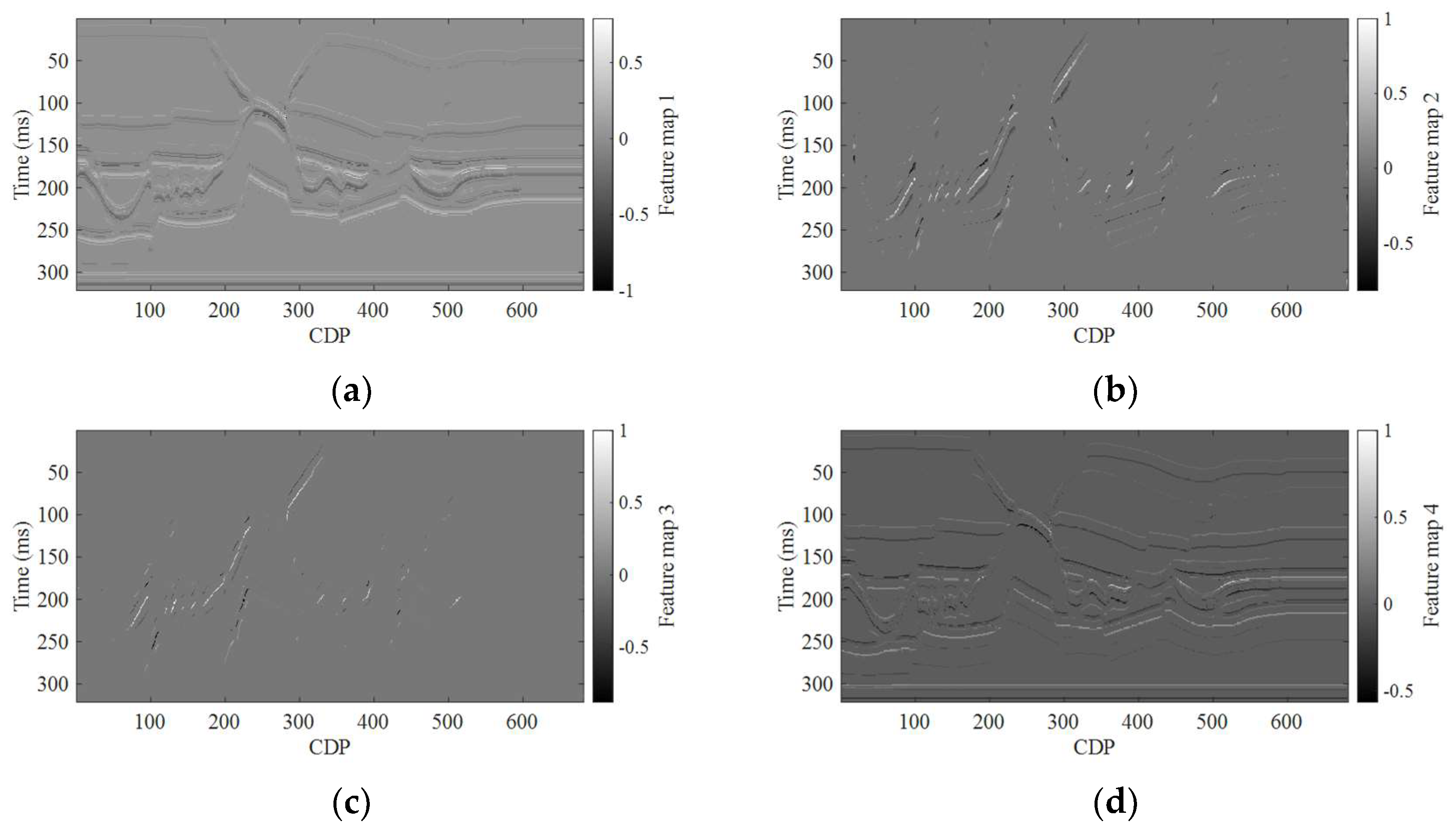
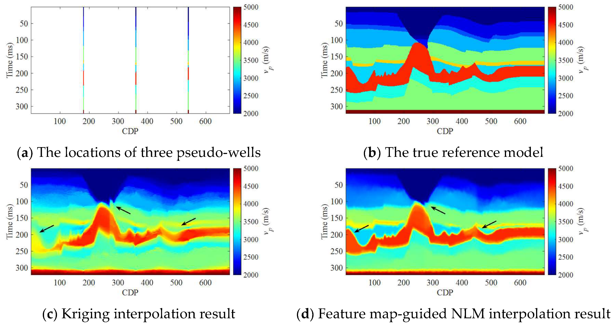
The clean poststack seismic record shown in Figure 4a is used for initial model building. The feature maps of different dictionary atoms can be obtained. We display four feature maps in Figure 6, which shows that each feature map can describe different subsurface structures. Compared with seismic data, there is no obvious bandlimited nature and noise interference. We use three pseudo-wells shown in Figure 7a and clean poststack seismic data for the initial model interpolation by FM-NLM as shown in Figure 7d. For comparison, we also display the interpolated results by kriging interpolation (KI) proposed by Yu et al. [33] shown in Figure 7c. Although KI can reveal weak variations in the shallow layers, it may introduce obvious abnormal values and structures which interferes seismic inversion and interpretation. In particular, at the edges of the high-velocity salt dome, there are finer contact relationships. Due to the direct use of band-limited seismic data, KI interpolation results always show biased model structures. FM-NLM utilizes the feature maps to construct the elastic parameter models, which can provide more accurate details. The interpolated result obtained by FM-NLM can reveal more accurate elastic parameter variations, and hold accurate amplitude even far away from the wells. We also list the REs and computational time for interpolations in Table 1. It can be seen that KI needs more computational time, which is hard to expand to 3D (three-dimensional) well-log interpolation.
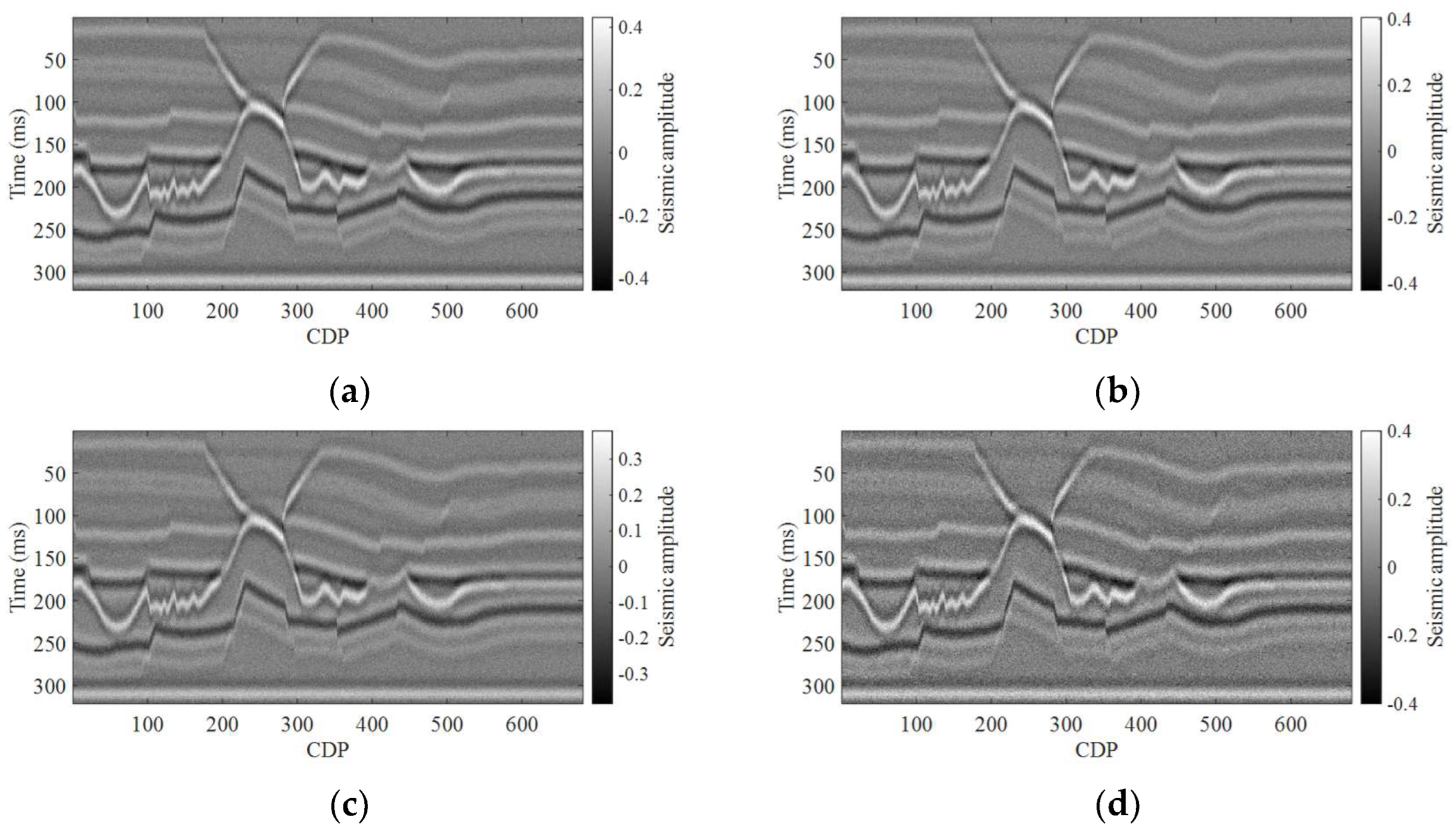
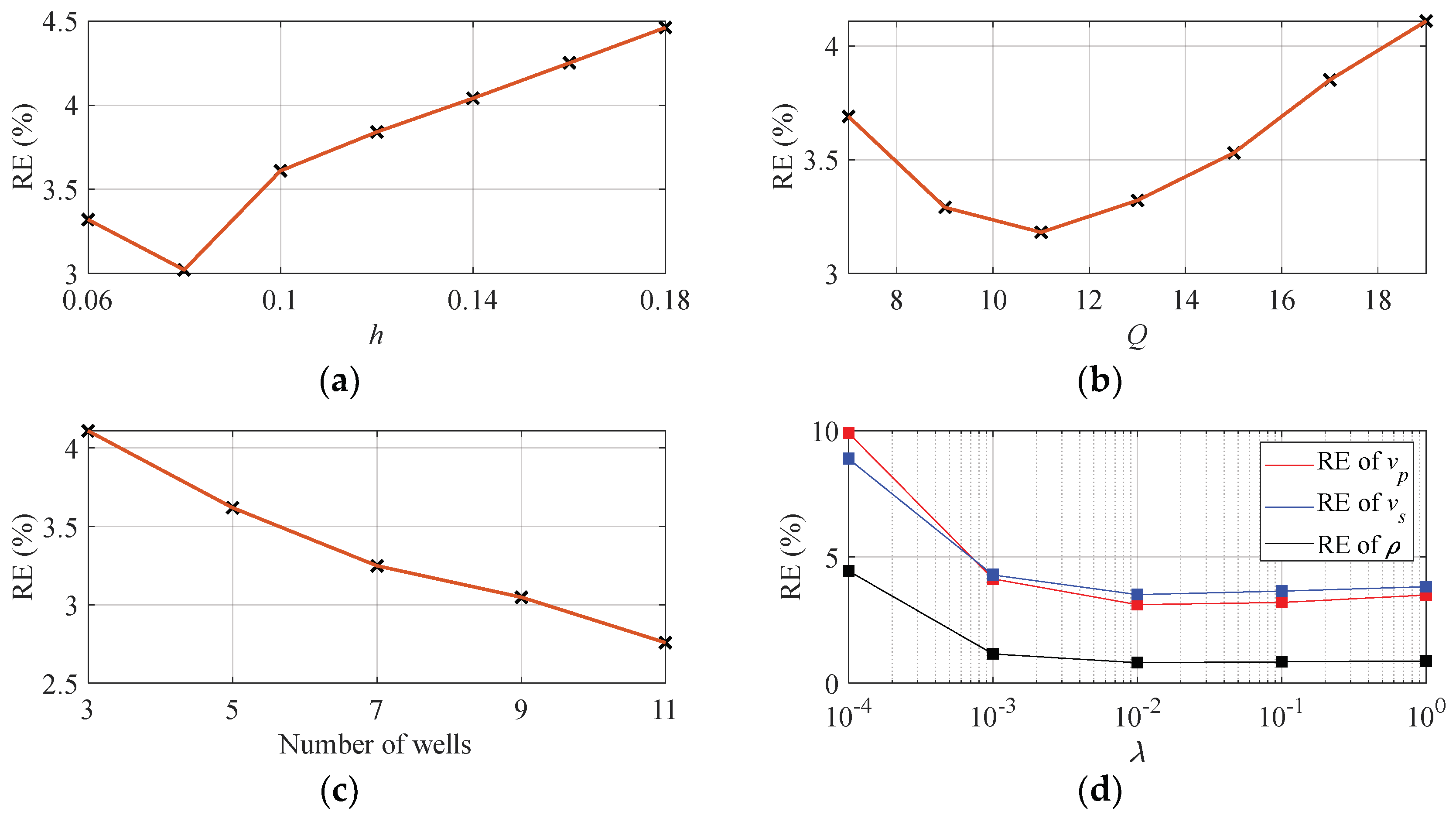
Then, the noisy poststack seismic records with snr = 2 shown in Figure 5d is used for initial model building. The interpolated results with three wells by KI and FM-NLM are shown in Figure 8c,d. Compared with the KI result, the FM-NLM interpolation result holds accurate amplitude variation, especially for the high-velocity salt dome, because KI interpolation is conducted based on the noisy observed seismic record. In contrast, FM-NLM utilizes the extracted feature maps from dictionary learning. Dictionary learning as an efficient denoising algorithm can preserve useful signal from noisy observed data. We test the influence of the number of wells and hyper-parameters for interpolation. Figure 9 shows the RE of interpolated results variation with hyper-parameter h, the numbers of reference points Q and wells, and inversion hyper-parameter λ. We can observe that RE becomes larger with the increase in h, since larger h makes interpolation weight coefficients similar contribution to the interpolated points. The interpolated result becomes smoother and obscure. In Figure 9b, smaller or larger Q leads to larger RE, since larger Q implies more reference points taken into interpolation and smaller Q cannot describe high-steep structures. As we know, more wells imply more known points for interpolation. Therefore, the interpolation accuracy increases with an increase in the number of known wells. We also test the accuracy of inversion results variation with λ. In Figure 9d, the red line, blue line, and black line represent REs of P-wave velocity, S-wave velocity, and density inversion results, respectively. When λ is smaller, the inversion results are sensitive to the noise presented in the observed seismic record. Conversely, the inversion results converge towards the initial model, which cannot depict subsurface details.
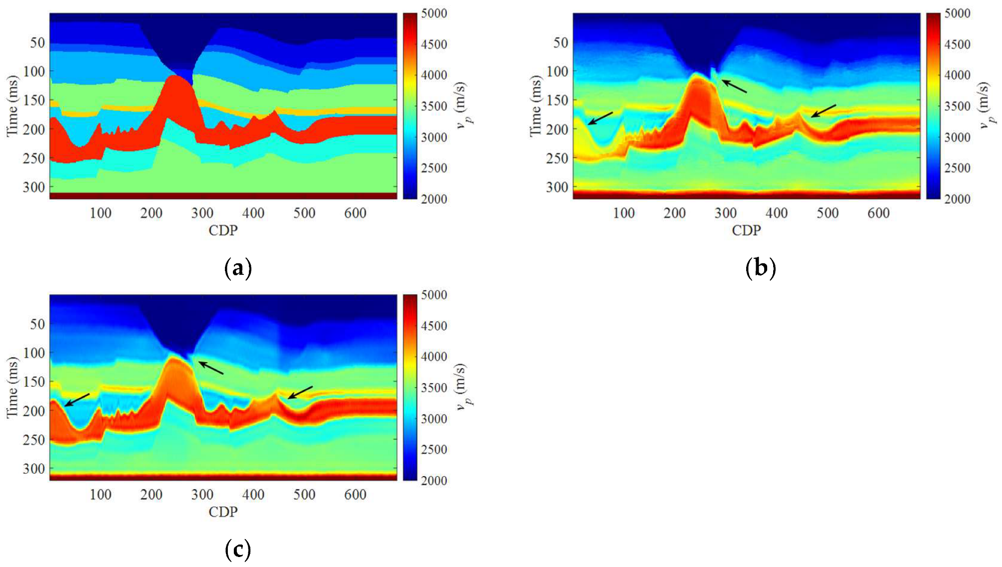
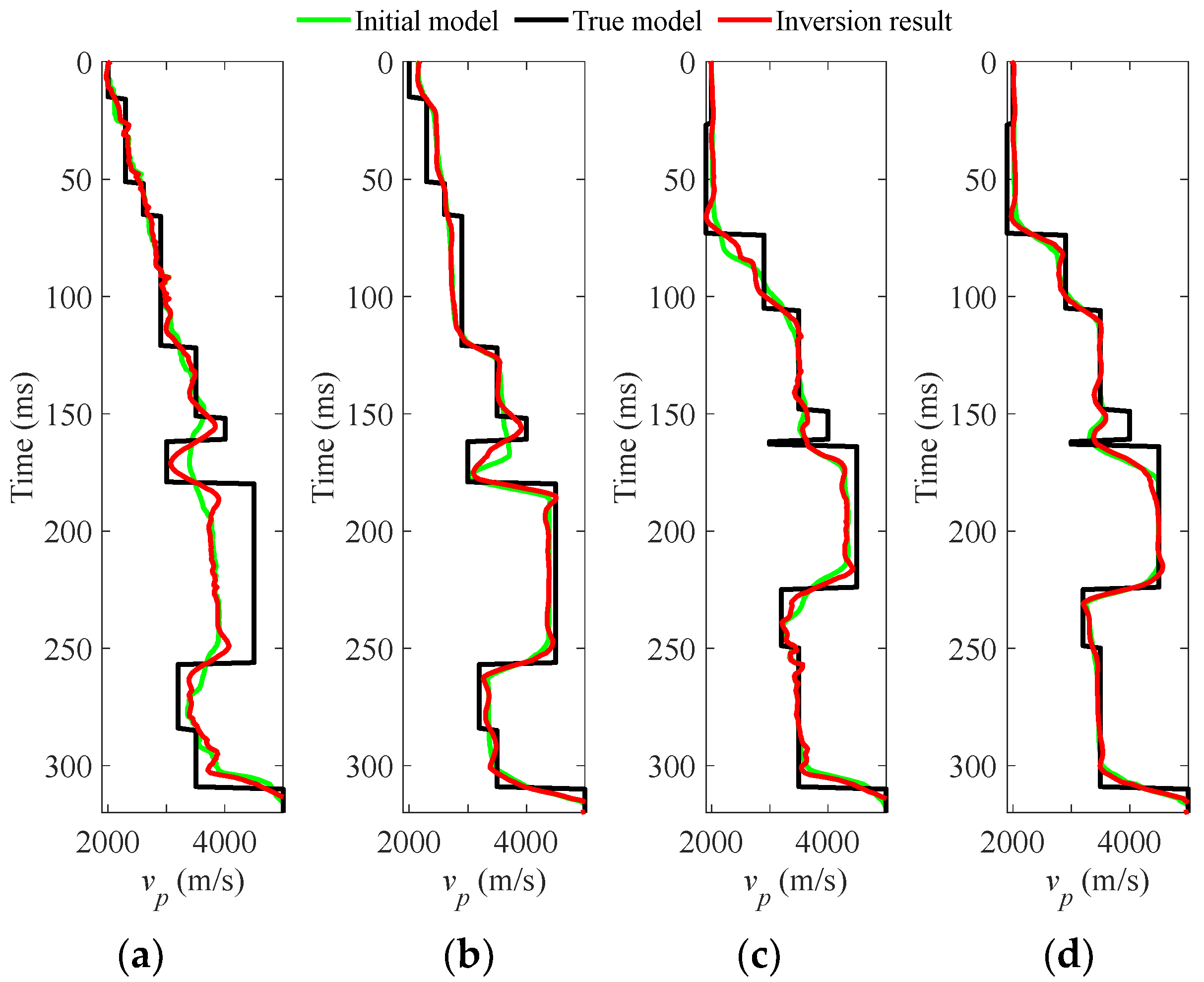
The prestack seismic inversion results are shown in Figure 10 by KI and FM-NLM interpolation results. In the KI-based inversion results, there are obvious amplitude deviation when CDPs are far away from the well locations, which indicates that model-driven inversion results are dependent on the initial model. In contrast, prestack inversion results using the initial model from FM-NLM can accurately depict the structure extension. To quantitatively evaluate the inversion results, we list REs of inversion results in Table 2. The inversion results by using the initial models from FM-NLM possess higher accuracy. We also plot P-wave velocity inversion results at CDPs 10 and 295 in Figure 11. The green, black, and red lines denote the initial model, the true model, and inversion results, respectively. At CDP 10, there are large deviations of inversion results using initial model by KI between 180 and 260 ms, with which it is hard to describe the accurate lateral variation of elastic parameters. Moreover, there are small jitters at shallow strata, which are caused by the noise presented in the observed seismic record. At CDP 295, it is also hard for KI-based inversion results to describe the amplitude of the high-velocity salt dome. In contrast, FM-NLM based inversion results can reveal accurate velocity variation at one stratum.

3.2. Field Data Example

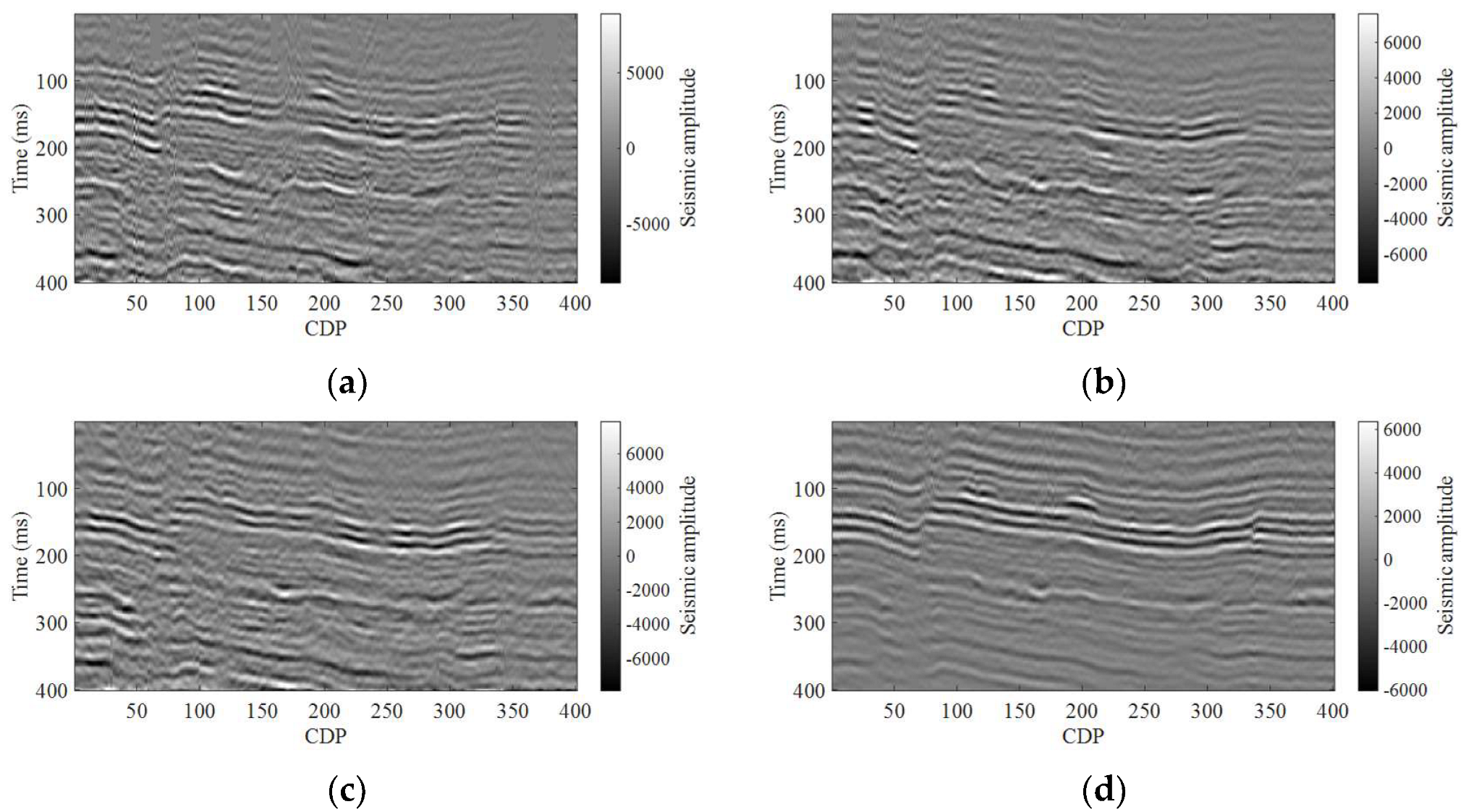
We also test the proposed method on a field data set. There are 401 CDPs and 401 sampling points at each CDP. The observed angle gathers of 0°, 15°, and 30° are shown in Figure 12a–c. The poststack seismic record is displayed in Figure 12d. There are three wells on this seismic profile, which are located at CDP 36, CDP 161, and CDP 304.
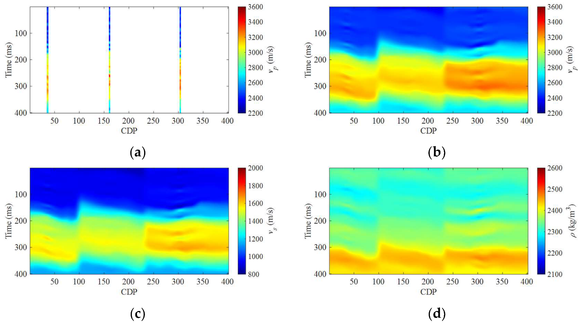
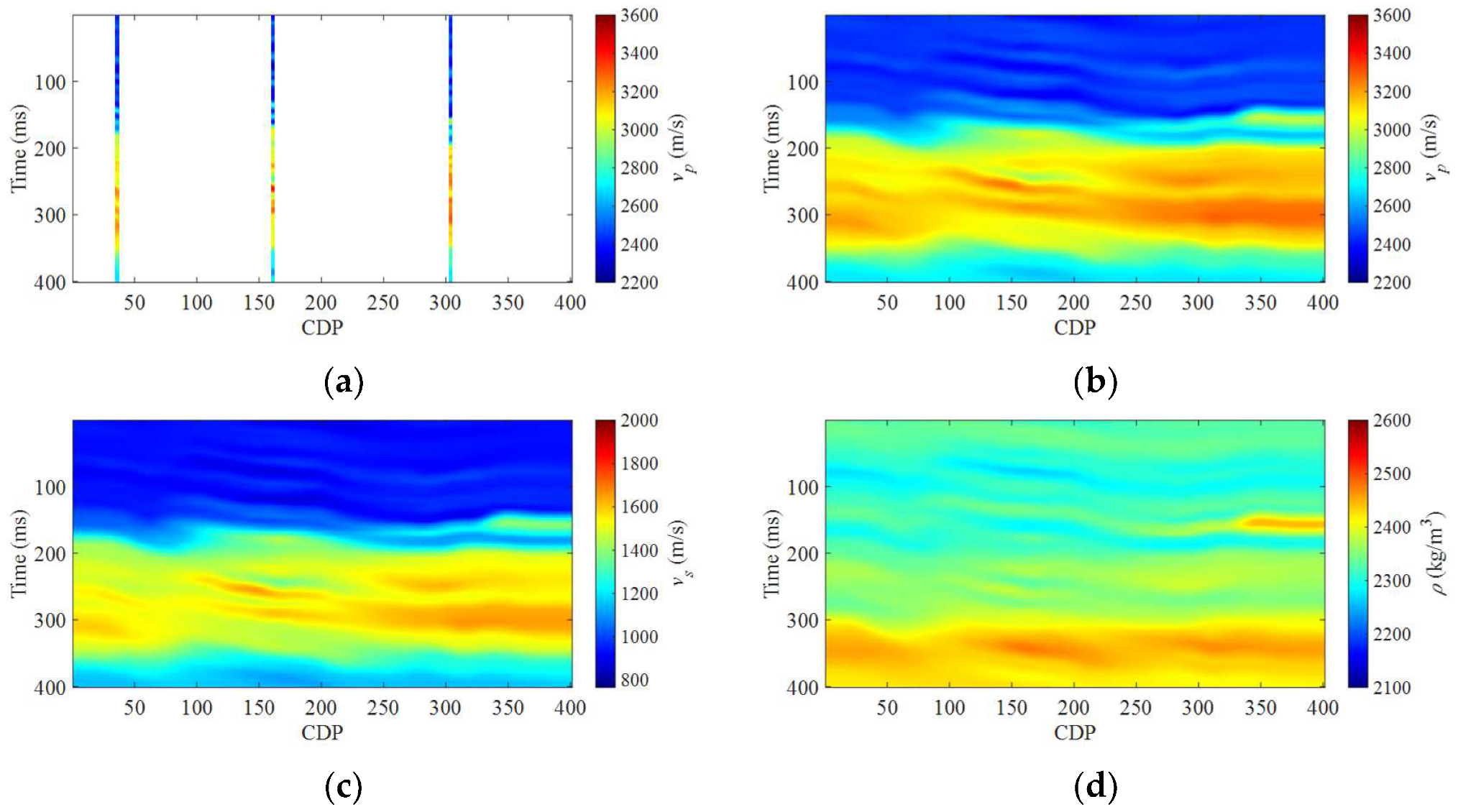
We use two wells at CDPs 36 and 304 for elastic parameters interpolation and show the interpolation results by KI and FM-NLM in Figure 13 and Figure 14, respectively. FM-NLM interpolation results show that there is a large fault located between CDP 50 and 100, which accurately matches the intuitive structure in the recorded poststack seismic record (Figure 12d). However, there are obvious two large faults and three block structure in traditional KI interpolation results. Between CDP 100 and 250, there are obvious resolution difference, which is caused by the smoother model far away from known wells by KI interpolation method. At locations of wells, the model variation is relatively dramatic compared with interpolated results far away from the wells.
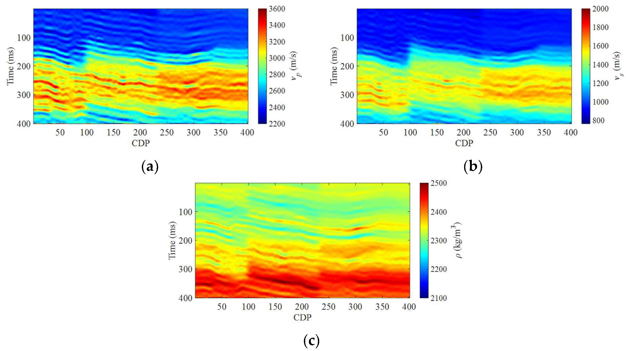
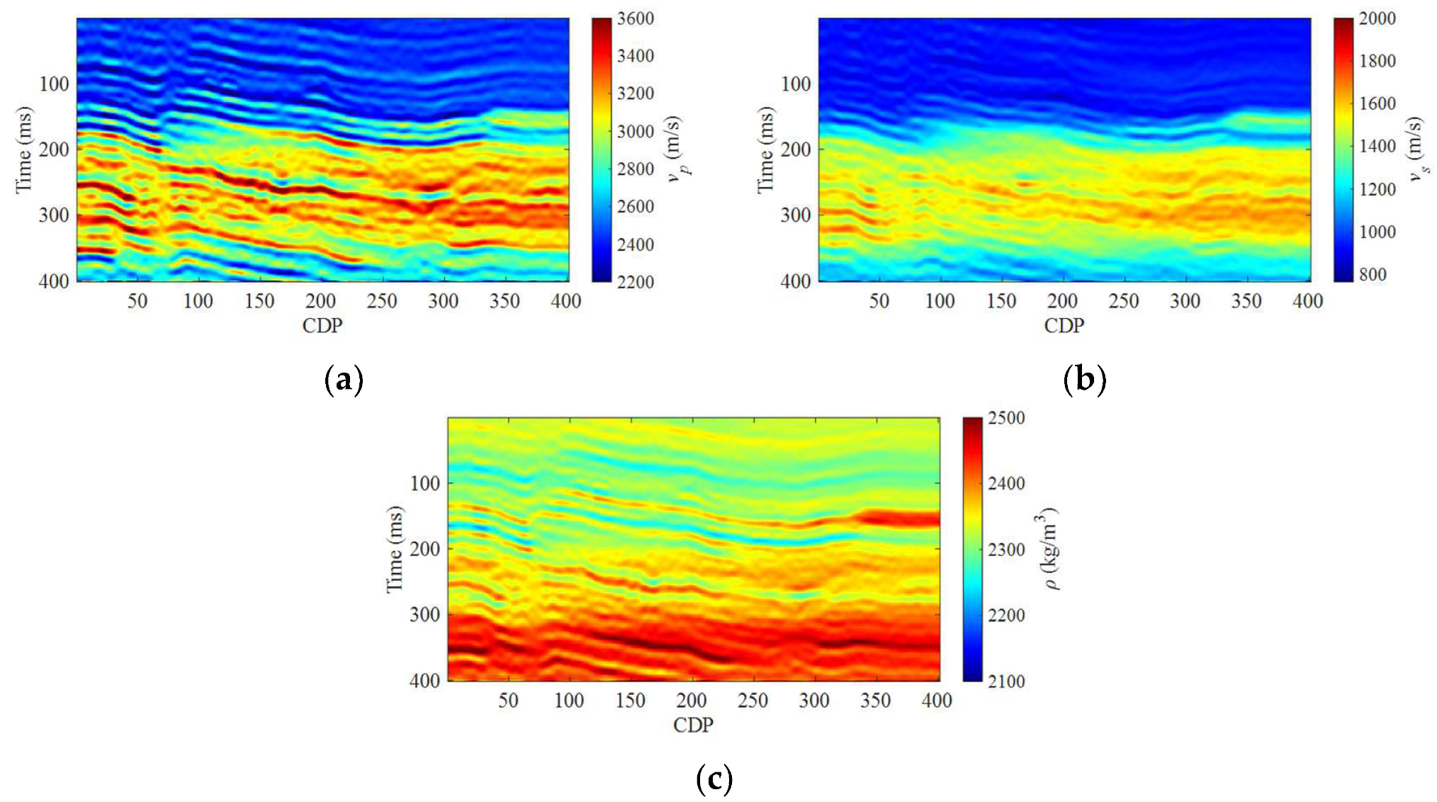
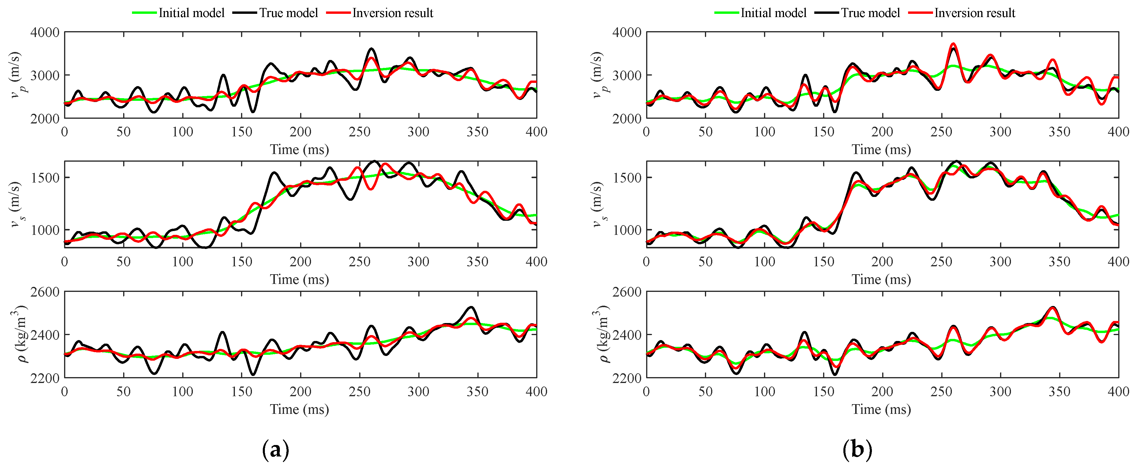
Then, these interpolated results are applied in model-driven prestack seismic inversion. The inversion results are shown in Figure 15 and Figure 16. The spatial extension of inversion results from different initial models is different. The inversion results from FM-NLM models hold better spatial continuity, and the spatial extension complies to the constructed initial model. Compared with the structure variation shown in poststack seismic record (Figure 12d), inversion results from FM-NLM models comfort to the geological situations. To evaluate the accuracy of the inversion results, we display the inversion results with the borehole data at CDP 161 in Figure 17. The original borehole data are processed by a 70–80 Hz low-pass filter. In Figure 17, the red, green, and black lines denote the inversion result, initial model, and borehole data, respectively. The REs of inversion results by KI models are 4.16%, 5.83%, and 0.96%. The REs of inversion results by FM-NLM models are 2.73%, 2.50%, and 0.37%. We can observe that the initial model and inversion results hold well variation tendency with the borehole data. There are more obvious mismatches for S-wave velocity, which may be caused by an inaccurate ratio between P- and S-wave velocities for prestack inversion [54].

4. Conclusions

In this paper, we have proposed an efficient adaptive well-log interpolation method for prestack seismic inversion. The proposed interpolation scheme includes feature map extraction and non-local means interpolation. Feature maps are extracted from the observed seismic profile with dictionary learning, which projects observed seismic data into dictionary atoms to record local features. The subsurface features are recorded in the form of dictionary atoms, and each sampling point can be represented as a sparse vector, which is defined as a feature map. Unlike conventional seismic-guided well-log interpolation, the proposed method adaptively selects feature maps from observed seismic data. The reliability of these feature maps can be demonstrated by the popularization of dictionary learning denoising. We use the sparse coefficients from dictionary learning as feature map, which can provide finer structure and possess clean information. Then, these features are used for non-local means interpolation to calculate interpolated weight coefficients. More similar feature maps imply the elastic parameters’ extension direction. To illustrate the necessity and practicability of initial model building, the interpolation results are used for model-driven prestack seismic inversion. To illustrate the performance of the proposed method, the conventional kriging interpolation method is used for comparison. In the synthetic test, the feature map guided interpolation and inversion results show more accuracy and efficiency compared with kriging interpolation based on relative error and computational time. In the field data test, the sparse borehole data are used for interpolation and prestack seismic inversion. Conventional kriging interpolation cannot describe model variation for interpolated points far away from wells, which always show smoother results. The inversion results are compared with known borehole data to evaluate the accuracy of inversion results. The field data test shows that compared with traditional kriging interpolation, inversion results from feature map-guided interpolation match better with borehole data. In future work, it is expected to extend the proposed method to a three-dimensional initial model building for fine characterization of underground structures.

Author Contributions

Conceptualization, L.W. and H.Z.; formal analysis, H.C.; investigation, H.C.; methodology, L.W.; resources, H.Z.; software, L.W.; supervision, H.Z. and H.C.; writing—original draft L.W.; writing—review and editing, H.Z. All authors have read and agreed to the published version of the manuscript.

Funding

This research was partly supported by National Key R&D Program of China (2018YFA0702502), R&D Department of CNPC (2022DQ0604-03), and the 14th 5-Year Prospective and Basic Research Program of CNPC (2021DJ3506).

Data Availability Statement

The data used in this study are available by contacting the corresponding author.

Conflicts of Interest

The authors declare no conflict of interest.

References

  1. Wang, L.; Zhou, H.; Wang, Y.; Yu, B.; Zhang, Y.; Liu, W.; Chen, Y. Three-parameter prestack seismic inversion based on L1-2 minimization. Geophysics 2019, 84, R753–R766. [Google Scholar] [CrossRef]
  2. Huang, G.; Chen, X.; Qu, S.; Bai, M.; Chen, Y. Directional Total Variation Regularized High-Resolution Prestack AVA Inversion. IEEE Trans. Geosci. Remote Sens. 2021, 60, 4502511. [Google Scholar] [CrossRef]
  3. Huang, G.; Chen, X.; Luo, C.; Chen, Y. Dynamic Characterization of Reservoirs Constrained by Time-Lapse Prestack Seismic Inversion. IEEE Trans. Geosci. Remote Sens. 2020, 59, 5549–5562. [Google Scholar] [CrossRef]
  4. Luo, C.; Ba, J.; Carcione, J. A Hierarchical Prestack Seismic Inversion Scheme for VTI Media Based on the Exact Reflection Coefficient. IEEE Trans. Geosci. Remote Sens. 2022, 60, 4507416. [Google Scholar] [CrossRef]
  5. Hamid, H.; Pidlisecky, A.; Lines, L. Prestack structurally constrained impedance inversion. Geophysics 2018, 83, R89–R103. [Google Scholar] [CrossRef]
  6. Karimi, O.; Omre, H.; Mohammadzadeh, M. Bayesian closed-skew Gaussian inversion of seismic AVO data for elastic material properties. Geophysics 2010, 75, R1–R11. [Google Scholar] [CrossRef] [Green Version]
  7. Pan, X.; Lu, C.; Zhang, G.; Wang, P.; Liu, J. Seismic Characterization of Naturally Fractured Reservoirs with Monoclinic Symmetry Induced by Horizontal and Tilted Fractures from Amplitude Variation with Offset and Azimuth. Surv. Geophys. 2022, 43, 815–851. [Google Scholar] [CrossRef]
  8. Buland, A.; Omre, H. Bayesian linearized AVO inversion. Geophysics 2003, 68, 185–198. [Google Scholar] [CrossRef] [Green Version]
  9. Buland, A.; Omre, H. Bayesian wavelet estimation from seismic and well data. Geophysics 2003, 68, 2000–2009. [Google Scholar] [CrossRef] [Green Version]
  10. Ahmed, N.; Weibull, W.; Grana, D. Constrained non-linear AVO inversion based on the adjoint-state optimization. Comput. Geosci. 2022, 16, 105214. [Google Scholar] [CrossRef]
  11. Zong, Z.; Wang, Y.; Li, K.; Yin, X. Broadband seismic inversion for low-frequency component of the model parameter. IEEE Trans. Geosci. Remote Sens. 2018, 56, 5177–5184. [Google Scholar] [CrossRef]
  12. Yuan, S.; Jiao, X.; Luo, Y.; Sang, W.; Wang, S. Double-scale supervised inversion with a data-driven forward model for low-frequency impedance recovery. Geophysics 2022, 87, R165–R181. [Google Scholar] [CrossRef]
  13. Yao, G.; Silva, N.; Warner, M.; Wu, D.; Yang, C. Tackling cycle skipping in full-waveform inversion with intermediate data. Geophysics 2019, 84, R411–R427. [Google Scholar] [CrossRef]
  14. Fang, J.; Zhou, H.; Li, Y.; Zhang, Q.; Wang, L.; Sun, P.; Zhang, J. Data-driven low-frequency signal recovery using deep-learning predictions in full-waveform inversion. Geophysics 2020, 85, A37–A43. [Google Scholar] [CrossRef]
  15. Gan, S.; Wang, S.; Chen, Y.; Qu, S.; Zu, S. Velocity analysis of simultaneous-source data using high-resolution semblance-Coping with the strong noise. Geophys. J. Int. 2016, 204, 768–779. [Google Scholar] [CrossRef] [Green Version]
  16. Taner, M.T.; Koehler, F. Velocity spectra-digital computer derivation applications of velocity functions. Geophysics 1969, 34, 859–881. [Google Scholar] [CrossRef]
  17. Fomel, S. Velocity analysis using ab semblance. Geophys. Prospect. 2009, 57, 311–321. [Google Scholar] [CrossRef] [Green Version]
  18. Zelt, C.A.; Barton, P.J. Three-dimensional seismic refraction tomography: A comparison of two methods applied to data from the Faeroe Basin. J. Geophys. Res. Solid Earth 1998, 103, 7187–7210. [Google Scholar] [CrossRef]
  19. Korenaga, J.; Holbrook, W.S.; Kent, G.M.; Kelemen, P.B.; Detrick, R.S.; Larsen, H.C.; Hopper, J.R.; Dahl-Jensen, T. Crustal structure of the southeast Greenland margin from joint refraction and reflection seismic tomography. J. Geophys. Res. Solid Earth 2000, 105, 21591–21614. [Google Scholar] [CrossRef]
  20. Noble, M.; Thierry, P.; Taillandier, C.; Calandra, H. High-performance 3D first-arrival traveltime tomography. Lead. Edge 2010, 29, 86–93. [Google Scholar] [CrossRef]
  21. Yuan, S.; Wang, S.; Luo, Y.; Wei, W.; Wang, G. Impedance inversion by using the low-frequency full-waveform inversion result as an a priori model. Geophysics 2019, 84, R149–R164. [Google Scholar] [CrossRef]
  22. Mallick, S.; Adhikari, S. Amplitude-variation-with-offset and prestack-waveform inversion: A direct comparison using a real data example from Rock Springs Uplift, Wyoming, USA. Geophysics 2015, 80, B45–B59. [Google Scholar] [CrossRef]
  23. Yao, G.; Silva, N.V.; Wu, D. Sensitivity analysis of acoustic impedance inversion with full-waveform inversion. J. Geophys. Eng. 2018, 15, 461–477. [Google Scholar] [CrossRef] [Green Version]
  24. Huang, G.; Chen, X.; Luo, C.; Chen, Y. Geological structure-guided initial model building for prestack AVO/AVA inversion. IEEE Trans. Geosci. Remote Sens. 2021, 59, 1784–1793. [Google Scholar] [CrossRef]
  25. Hampson, D.P.; Schuelke, J.S.; Quirein, J.A. Use of multiattribute transforms to predict log properties from seismic data. Geophysics 2001, 66, 220–236. [Google Scholar] [CrossRef]
  26. Nivlet, P. Low-Frequency Constrain in a Priori Model Building for Stratigraphic Inversion; SEG Technical Program Expanded Abstracts; Society of Exploration Geophysicists: Houston, TX, USA, 2004; pp. 1802–1805. [Google Scholar]
  27. Hansen, T.K.; Mosegaard, K.; Pedersentatalovic, R.; Uldall, A.; Jacobsen, N.L. Attribute-guided well-log interpolation applied to low-frequency impedance estimation. Geophysics 2008, 73, R83–R95. [Google Scholar] [CrossRef] [Green Version]
  28. Ray, A.K.; Chopra, S. Building more robust low-frequency models for seismic impedance inversion. First Break 2016, 34, 47–52. [Google Scholar]
  29. Chen, Y.; Chen, X.; Wang, Y.; Zu, S. The interpolation of sparse geophysical data. Surv. Geophys. 2019, 40, 73–105. [Google Scholar] [CrossRef]
  30. Naeini, E.Z.; Hale, D. Image- and horizon-guided interpolation. Geophysics 2014, 80, V47–V56. [Google Scholar] [CrossRef] [Green Version]
  31. Wu, X. Building 3D subsurface models conforming to seismic structural and stratigraphic features. Geophysics 2017, 82, IM21–IM30. [Google Scholar] [CrossRef] [Green Version]
  32. Chen, Y.; Chen, H.; Xiang, K.; Chen, X. Geological structure guided well log interpolation for high-fidelity full waveform inversion. Geophys. J. Int. 2016, 207, 1313–1331. [Google Scholar] [CrossRef]
  33. Yu, B.; Zhou, H.; Liu, W.; Wang, L.; Chen, H. Interpolation method based on pattern-feature correlation. Geophysics 2021, 86, R253–R264. [Google Scholar] [CrossRef]
  34. Wang, X.; Ma, J. Adaptive dictionary learning for blind seismic data denoising. IEEE Geosci. Remote Sens. Lett. 2020, 17, 1273–1277. [Google Scholar] [CrossRef]
  35. Kuruguntia, L.; Dodda, V.C.; Elumalai, K. Study of parameters in dictionary learning method for seismic denoising. IEEE Trans. Geosci. Remote Sens. 2022, 60, 5906213. [Google Scholar]
  36. Liu, L.; Ma, J. Structure graph dictionary learning and application on the seismic denoising. IEEE Trans. Geosci. Remote Sens. 2019, 57, 1883–1893. [Google Scholar] [CrossRef]
  37. Chen, Y. Fast dictionary learning for noise attenuation of multidimensional seismic data. Geophys. J. Int. 2020, 222, 1717–1727. [Google Scholar] [CrossRef]
  38. Zu, S.; Zhou, H.; Wu, R.; Jiang, M.; Chen, Y. Dictionary learning based on dip patch selection training for random noise attenuation. Geophysics 2019, 84, V169–V183. [Google Scholar] [CrossRef]
  39. Zu, S.; Zhou, H.; Wu, R.; Mao, W.; Chen, Y. Hybrid-sparsity constrained dictionary learning for iterative deblending of extremely noise simultaneous-source data. IEEE Trans. Geosci. Remote Sens. 2019, 57, 2249–2262. [Google Scholar] [CrossRef]
  40. Yu, S.; Ma, J.; Zhang, X.; Sacchi, M. Interpolation and denoising of high-dimensional seismic data by learning a tight frame. Geophysics 2015, 80, V119–V132. [Google Scholar] [CrossRef]
  41. Zhi, L.; Chen, S.; Li, X. Amplitude variation with angle inversion using the exact Zoeppritz equations-theory and methodology. Geophysics 2016, 81, N1–N15. [Google Scholar] [CrossRef]
  42. Aki, K.; Richards, P.G. Quantitative Seismology: Theory and Methods; W. H. Freeman: San Francisco, CA, USA, 1980. [Google Scholar]
  43. Yilmaz, O. Seismic Data Analysis: Processing, Inversion, and Interpretation of Seismic Data; SEG: Tulsa, OK, USA, 2001; Volume 1. [Google Scholar]
  44. Stolt, R.H.; Weglein, A.B. Migration and inversion of seismic data. Geophysics 1985, 50, 2458–2472. [Google Scholar] [CrossRef] [Green Version]
  45. Russell, B.; Hampson, D. Comparison of Post-Stack Seismic Inversion Methods; SEG Technical Program Expanded Abstracts; Society of Exploration Geophysicists: Houston, TX, USA, 1991; pp. 876–878. [Google Scholar]
  46. Huang, J.B.; Singh, A.; Ahuja, N. Single image super-resolution from transformed self-exemplars. In Proceedings of the 2015 IEEE Conference on Computer Vision and Pattern Recognition (CVPR), Boston, MA, USA, 7–12 June 2015; pp. 5197–5206. [Google Scholar]
  47. Jiang, J.; Ma, X.; Chen, C.; Lu, T.; Wang, Z.; Ma, J. Single image super-resolution via locally regularized anchored neighborhood regression and nonlocal means. IEEE Trans. Multimed. 2017, 19, 15–26. [Google Scholar] [CrossRef]
  48. She, B.; Wang, Y.; Liu, Z.; Cai, H.; Liu, W.; Hu, G. Seismic impedance inversion using dictionary learning-based sparse representation and nonlocal similarity. Interpretation 2019, 7, SE51–SE67. [Google Scholar] [CrossRef]
  49. Dong, W.; Zhang, L.; Shi, G.; Li, X. Nonlocally centralized sparse representation for image restoration. IEEE Trans. Image Process. 2013, 22, 1620–1630. [Google Scholar] [CrossRef] [PubMed] [Green Version]
  50. Rubinstein, R.; Zibulevsky, M.; Elad, M. Efficient implementation of the K-SVD algorithm using batch orthogonal matching pursuit. Technion 2008, 40, 1–15. [Google Scholar]
  51. Rubinstein, R.; Zibulevsky, M.; Elad, M. Double sparsity: Learning sparse dictionaries for sparse signal approximation. IEEE Trans. Signal Process. 2010, 58, 1553–1564. [Google Scholar] [CrossRef]
  52. Aharon, M.; Elad, M.; Bruckstein, A. K-SVD: An algorithm for designing overcomplete dictionaries for sparse representation. IEEE Trans. Signal Process. 2006, 54, 4311–4322. [Google Scholar] [CrossRef]
  53. Elad, M.; Aharon, M. Image denoising via sparse and redundant representations over learned dictionaries. IEEE Trans. Image Process. 2006, 15, 3736–3745. [Google Scholar] [CrossRef]
  54. Wang, L.; Zhou, H.; Yu, B.; Chen, H.; An, Y.; Huang, W. The Analysis of the Influence of Vs/Vp on the Elastic Impedance Inversion. In Proceedings of the 81st EAGE Conference and Exhibition, London, UK, 3–6 June 2019; pp. 1–5. [Google Scholar]
Figure 1. The schematic diagram for obtaining NLM interpolation coefficients based on the observed poststack seismic record. (a) The elastic parameters for interpolation (green circle) and the known points (yellow circle) at well location (blue line), and (b) seismic patches centered at borehole points (yellow rectangle) and interpolated point (green rectangle) are used to calculate the interpolation weight coefficients bi,j,q.
Remotesensing 15 00459 g001
Figure 2. (a) Synthetic poststack seismic data and (b) some seismic patches decomposed from the seismic profile with a sliding window.
Remotesensing 15 00459 g002
Figure 3. The schematic diagram for obtaining NLM interpolation coefficients based on feature map. (a) The feature map from the fourth element in sparse vector, (b) feature maps of borehole points (yellow rectangle) and interpolated point (green rectangle) are used to calculate the interpolation weight coefficients bi,j,q.
Remotesensing 15 00459 g003
Figure 4. (a) The synthetic clean observed poststack seismic record, (b) true P-wave velocity of the salt dome intrusion model.
Remotesensing 15 00459 g004
Figure 5. The observed noisy prestack angle gathers of (a) 0°, (b) 15°, and (c) 30° for seismic inversion. (d) The noisy poststack seismic record used for initial model building.
Remotesensing 15 00459 g005
Figure 6. The feature maps from the (a) fifth, (b) tenth, (c) fifteenth, and (d) twentieth elements in sparse vector used for interpolation.
Remotesensing 15 00459 g006
Figure 7. The interpolation results from clean seismic record.
Remotesensing 15 00459 g007aRemotesensing 15 00459 g007b
Figure 8. The interpolation results from noisy seismic records.
Remotesensing 15 00459 g008
Figure 9. RE variation with (a) interpolation hyper-parameter h, (b) the number of reference points Q, (c) the number of wells, and (d) inversion hyper-parameter λ.
Remotesensing 15 00459 g009
Figure 10. Prestack seismic inversion results of vp, (a) reference model, (b) inversion result by KI model, (c) inversion result by FM-NLM.
Remotesensing 15 00459 g010
Figure 11. Prestack seismic inversion results of P-wave velocity at CDP 10 by (a) KI model and (b) FM-NLM, and inversion results at CDP 295 by (c) KI model and (d) FM-NLM.
Remotesensing 15 00459 g011
Figure 12. The observed prestack angle gathers of (a) 0°, (b) 15°, and (c) 30° for seismic inversion. (d) The poststack seismic record used for interpolation.
Remotesensing 15 00459 g012
Figure 13. (a) The locations of three wells and interpolation results of (b) vp, (c) vs, and (d) ρ by KI.
Remotesensing 15 00459 g013
Figure 14. (a) The locations of three pseudo-wells and interpolation results of (b) vp, (c) vs, and (d) ρ by FM-NLM.
Remotesensing 15 00459 g014
Figure 15. Prestack seismic inversion results of (a) vp, (b) vs, and (c) ρ by using the initial models shown in Figure 13 from KI.
Remotesensing 15 00459 g015
Figure 16. Prestack seismic inversion results of (a) vp, (b) vs, and (c) ρ by using the initial models shown in Figure 14 from FM-NLM.
Remotesensing 15 00459 g016
Figure 17. The comparison between the borehole data and the inversion results of vp, vs, and ρ by (a) KI models and (b) FM-NLM models.
Remotesensing 15 00459 g017
Table 1. The computational time and REs for interpolations.
KIFM-NLM
Time (s)1048205
RE3.93%1.75%
Table 2. The REs of prestack seismic inversion results.
vpvsρ
KI-based inversion3.93%4.72%1.01%
FM-NLM based inversion3.41%3.79%0.86%
Disclaimer/Publisher’s Note: The statements, opinions and data contained in all publications are solely those of the individual author(s) and contributor(s) and not of MDPI and/or the editor(s). MDPI and/or the editor(s) disclaim responsibility for any injury to people or property resulting from any ideas, methods, instructions or products referred to in the content.