Guidance-Aided Triple-Adaptive Frost Filter for Speckle Suppression in the Synthetic Aperture Radar Image

Abstract

Speckle noise exists inherently in the synthetic aperture radar (SAR) image. Its multiplicative property leads to lots of difficulties in SAR image processing. A novel guidance-aided triple-adaptive Frost filter is proposed in this paper, which has potential for real-time processing platforms. Firstly, a scale-adaptive sliding window sizing method is adopted to determine the neighborhood ranges for every point in the image. All the subsequent processing is based on it. Then, an adaptive calculation for the tuning factor in the Frost filter is embedded into the proposed method. Lastly, the feature information apertured from the original image is used to provide guidance for edge recovery automatically, which guarantees the satisfactory ability for feature preservation. Thus, a novel improved Frost filter is proposed with triple adaptabilities. Both the positioning accuracy and response sensitivity of the scale-adaptive sliding window sizing method are verified first. The superiority of the adaptive tuning factor combined with the scale-adaptive sliding window is confirmed by two comparison experiments. At last, the results of speckle suppression experiments on the synthetic images and two natural airborne SAR images present a better performance than other methods.

1. Introduction

Synthetic aperture radar (SAR) is well known as an active coherent imaging system, which works at all times and in all weather [1,2]. However, the SAR image seriously suffers from the multiplicative speckle noise, which is multiplicative and locally correlated. Therefore, the fluctuations of pixel intensity caused by the speckle are larger in the region where reflection intensity is higher, and vice versa [3]. For example, there is a speckled synthetic image and two natural Ku-band airborne SAR images (acquired in October 2020), presented in Figure 1. It can be noticed in Figure 1a that many dark pixels are interspersed in the center square region irregularly, where mean intensity is high, while no distribution of high-intensity pixels is present in the dark region. The reason for this phenomenon is the special multiplicative property of speckle, i.e., for a noiseless image $I$, the speckle noise $\xi$ acts on it in the manner $I_0=\xi \cdot I$, where $I_0$ is the captured original image. Consequently, for the SAR image, the stronger the reflection, the more fluctuating the pixel intensity is. The gradient, as the significant evidence for denoising and detection, bears the brunt of the impact from speckle. This means that larger gradients in the SAR image would appear not only at the edge (such as the situation in the optical image), but also in the regions with high reflection, which can be corroborated by Figure 1b,c.

There are a large number of speckle suppression methods that were proposed in past decades [4,5,6,7,8,9,10,11,12,13]. A case for classifying de-speckling methods according to the processing domain can be found in [4], in which they are categorized into spatial domain ones and transform domain ones. The huge amount of operations caused by transform and anti-transform operations constrains the applications of these transform domain methods in real-time. On the other hand, due to extensive research, the spatial domain ones developed into many well-established branches, such as the de-speckling methods, which are based on the non-local mean [5,6], total variation model [7], diffusion model [8,9,10,13], low-rank matrix approximation [11], etc. In addition, the advancement of machine learning (ML) techniques provided new ways to perform the above types of methods [12,14,15]. Regretfully, the ML-based methods are not interpretable mathematically; meanwhile, they are very sample-dependent, leading to their non-applicability for real-time applications. Although there are many reports about accelerating ML methods via some hardware processers, most of them just utilize the processers to speed a segment of the ML method (especially the training sessions) [16]. There are still little examples of applications that can be implemented entirely based on the hardware platforms. Therefore, in the rest of this paper, we mainly consider the speckle suppression methods in the spatial domain.

Frost filter, as one of the representative and classical speckle suppression methods, is proposed to enhance the coherent radar image, due to the standard image processing techniques being only applicable to noncoherent optically produced images [17]. By using locally estimated parameter values, the filter is made adaptive so that it provides minimum mean square error estimates inside homogeneous areas of an image while preserving the edge structure. However, the original Frost filter takes no consideration of parameter estimation with the scale space theory that provides guidance for parameter estimation or feature detection applications [18,19,20,21]. It would lead to the non-optimal smoothness controlled with the parameter values estimated in the fixed-size neighborhood centered at the current point. Nonetheless, there is still no authoritative way to determine the scale parameters for the space theory. The traditional scale space method is very computationally intensive, which does not facilitate its use in rudimentary or real-time requirements [8,18]. Therefore, the determination of scale parameters by a method other than image scale space is of great significance for effective computing. On the other hand, besides the guidance for filter parameter determination from scale parameter, the guidance for feature preservation is meaningful as well. The rolling guidance filter (RGF) method offers an approach to take feature information to keep edges sharpened in the image, which is called edge recovery in [22]. The RGF obtains edge information in the Gaussian difference scale space with the difference-based calculation method, which causes a high false alarm in the SAR image.

In this paper, an improved Frost filter is proposed. First, two guidance methods are adopted to achieve the parameter optimization for the proposed filter. One is the scale guidance for a size-adaptive neighborhood (i.e., sliding window) with the low memory footprint method, and the other is the edge guidance for accurate feature preservation. On the one hand, the more reliable filtering parameter is auto-calculated in the aforementioned size-adaptive neighborhood. On the other hand, we add an edge-guided feature-preserving term into the original filtering parameter. Both of the guidance improves the adaptability of the Frost filter. Lastly, an adaptive tuning factor method is adopted in our method. Since the proposed method is easy to implement, it has the potential to be applied to real-time processing platforms. We named the proposed method as a guidance-aided triple-adaptive Frost filter.

The remainder of this paper is organized as follows: Section 2 firstly introduces some related works with adaptive technology for speckle suppression. Later, the proposed guidance-aided size-adaptive Frost filter is described in detail. Section 3 presents the assignments of experiments, so that the considerations on the function validation of the proposed method and the de-speckling performance are more easily understood. The corresponding experimental results are shown in Section 3. Section 4 discusses the performance of our method. Finally, the conclusion is drawn in Section 5.

2. Backgrounds, Related Works, and Methods

2.1. Backgrounds and Related Works

All of the speckle suppression methods aim to smooth out the fluctuations of pixels caused by noise while maintaining sharp edges in the image. There are many methods proposed for speckle filtering along with feature protection. Roughly classified, two kinds of mainstream methods are used for spatial domain de-speckling, i.e., the anisotropic diffusion model-based ones and the feature detection-based ones. Three parts are included in this Section, such as an introduction to the anisotropic diffusion model-based method, the framework of RGF, and the scale space theory. On the one hand, the anisotropic diffusion model can be used as a reference to contrast with the subsequent methods in this paper. On the other hand, the RGF and scale space theory are the backgrounds of the proposed method with which it is possible to understand our method more clearly. More details are shown as follows.

2.1.1. Anisotropic Diffusion Model-Based Method

Perona and Malik [8,13] proposed the following nonlinear partial differential equation for smoothing images on the continuous domain:

$$\{\begin{array}{l}\frac{\partial I}{\partial t}=div\left[c\left(\left|\nabla I\right|\right)\cdot \nabla I\right]\\ I_0=I\end{array}$$

(1)

where $\nabla$ is the gradient operator, $div$ the divergence operator, $|\cdot |$ denotes the magnitude, $c(\cdot )$ the diffusion coefficient, and $I$ the initial image. There are two diffusion coefficients suggested,

$$c(x)=\frac{1}{1+{(x/k)}^2}$$

(2)

and

$$c(x)=\exp \left[-{(x/k)}^2\right]$$

(3)

where $k$ is an edge magnitude parameter. According to (2) and (3), it can be found that the diffusion coefficient value is determined by the relative magnitude of $x$ and $k$. For the anisotropic diffusion method, it turns to be an all-pass filter while $\left|\nabla I\right|\gg k$, and a mean filter while $\left|\nabla I\right|\ll k$. In other words, it only filters in uniform regions and does nothing at the edge. As Figure 2 shows, taking the region in the red box in Figure 1a as an example, anisotropic diffusion would only occur inside region 1 and region 2.

There is an iterative solution for (1) with the gradient descent method, which can be expressed as

$$\{\begin{array}{l}{I}_{n+1}=I_n+\Delta t\cdot div\left\{\left|\nabla I\right|/\left[1+\left(\left|\nabla I\right|/c(|\nabla I|)\right)\right]\right\}\\ I_0=I\end{array}$$

(4)

where $\Delta t$ represents the step size. However, the step size in anisotropic diffusion model-based method cannot be too large, which is usually set to 0.01~0.03 [9,10]. There are many variants based on the anisotropic diffusion model, such as the speckle reduction anisotropic diffusion (SRAD) [10] and quantitative anisotropic diffusion filter [4].

2.1.2. Framework of the Rolling Guidance Filter

With the advent of the RGF, it attracts lots of attention by its novel guidance-based framework for image denoising. Although the initial RGF only takes the additive noise model into consideration, the algorithm structure of RGF is very promising for improvement [22].

There are two main steps in the RGF method; that is, small structure removal and edge recovery. The Gaussian filter is related to determining the structure scale, which can be expressed as a weighted average form, i.e.,

$$G(p)=\frac{1}{W_p}{\displaystyle \sum _{q\in \mathbb{N}(p)}I(q)\cdot \exp \left(-{\Vert p-q\Vert }^2/2{\sigma }_s^2\right)}$$

(5)

where $q$ is the point in neighborhood $N(p)$ centered at $p$, ${\sigma }_s$ is the parameter of the Gaussian filter, $G$ is the output image, and $W_p={\displaystyle {\sum }_{q\in N(p)}\exp \left(-{\Vert p-q\Vert }^2/{\sigma }_s^2\right)}$ is the normalization coefficient. After removing small structures as well as noise in the image, the edge recovery is conducted by introducing a feedback factor into (5) in an iterative joint bilateral filtering form, which is given by

$$\{\begin{array}{l}{I}_{n+1}(p)=\frac{1}{K_p}{\displaystyle \sum _{q\in \mathbb{N}(p)}{I}_n(q)\cdot \exp \left[-{\Vert p-q\Vert }^2/2{\sigma }_s^2-{\Vert I_n(q)-I_n(p)\Vert }^2/2{\sigma }_r^2\right]}\\ I_0=I\end{array}$$

(6)

where

$$K_p={\displaystyle \sum _{q\in \mathbb{N}(p)}\exp \left[-{\Vert p-q\Vert }^2/2{\sigma }_s^2-{\Vert I_n(q)-I_n(p)\Vert }^2/2{\sigma }_r^2\right]}$$

is for normalization, and ${\sigma }_r$ controls the range weight. It can be found that the feedback factor is calculated in a difference-based way. As mentioned above, for SAR image processing, where the multiplicative noise is inevitable, there is a high false alarm rate in the difference-based result. Consequently, many variants based on the framework of RGF are designed, such as the edge-aware superpixel generation method [23] and the improved RGF for SAR image (SAR-IRGF) [24].

2.1.3. Overview of the Scale Space Theory

The scale space theory is proposed to solve the problem of extracting image features at various scales in the field of image processing [20], and was widely applied to image registration [2,25], target detection [26,27], and so on. The Gaussian scale space is one of the most commonly used scale spaces, which is obtained by successive convolution of the image via Gaussian functions with various scale parameters. A simple example of Gaussian scale space built based on the subregion in Figure 1b is shown in Figure 3, from which it can be seen that the noise and detailed features of the image gradually disappear as the scale parameter increases. Accordingly, ones could know intuitively that the scale space theory aims to obtain the mapping between various features and scale parameters.

However, the authoritative method for determining the scale is not confirmed yet. Furthermore, applications of scale space theory are computationally expensive, resulting in the limitation of some real-time processing tasks. Therefore, there is a demand for scale determination methods other than scale space theory-based methods.

Markdown: The anisotropic diffusion model-based methods present a de-speckling view different from the proposed method, and SRAD as a representative of them will be selected as the comparison method in Section 3. With the introduction of RGF and scale space theory, their core ideas will both be integrated into the proposed method, as will be shown later.

2.2. Guidance-Aided Triple-Adaptive Frost Filter

Based on the framework of RGF, a triple-adaptive Frost filter is proposed for de-speckling. Firstly, the determination of scale parameters independent of the scale space theory-based methods is adopted for the scale-adaptability in this paper. This scale-adaptive method can produce a suitable size for the neighborhood centered at each pixel, which makes the filtering parameters obtained in a proper range. Next, the tuning factor, which is important but not easy to predefine in the Frost filter, is computed adaptively using the regional characteristics and the values of region pixels simultaneously. Lastly, referring to the idea of edge recovery in RGF, we design an edge guidance factor that is applicable to SAR images for adaptive feature preservation. More details about the proposed method are as follows.

2.2.1. Traditional Frost Filter

The Frost filter is first proposed in [17], which is based on the minimum mean square error criterion. There are two preconditions for the designing of the Frost filter, i.e., the speckle noise is multiplicative, and the SAR image is stationary [17,28,29]. In particular, the Frost filter does not own a simple linear weighted form of the real image and the observed image. The original Frost filter can be expressed as

$$I^{\mathrm{Frost}}(p)=\frac{1}{M_p}{\displaystyle \sum _{q\in \mathbb{N}(p)}I(q)\cdot \exp \left(-\kappa {\Vert p-q\Vert }^2{C}_q^2\right)}$$

(7)

in which $I^{\mathrm{Frost}}$ is the output of the Frost filter, $\kappa (\kappa >0)$ denotes the tuning factor, $C_q$ represents the coefficient of the variation at $q$ that is defined by the ratio of the sample standard deviation to the average of the sample, and $M_p={\displaystyle {\sum }_{q\in \mathbb{N}(p)}\exp \left(-\kappa {\Vert p-q\Vert }^2{C}_q^2\right)}$ is the normalization coefficient. The coefficient of variation is related to the extent to which the image is affected by noise. Consequently, it can be found from (7) that Frost reduces speckle noise more thoroughly in the homogeneous regions where values of $C_q$ are smaller, and vice versa.

2.2.2. Scale-Adaptive Size for the Neighborhood

Due to high memory usage for building image scale space, another way to determine the neighborhood size is adopted in this paper. We noticed that the coefficient of variation mentioned in the Frost filter is not bound by measurement scale and dimension to describe the dispersion degree of various data. Accordingly, it is possible to estimate whether any point is near the edge.

Supposing there is a square neighborhood, centered at $(x,y)$, with width $d_{(x,y)}$, then one can utilize the coefficient of variation that is gathered using pixels at the boundary $\mathbb{B}$ of the current range as the evidence to decide the neighborhood size at the next position. It can be mathematically formulated as

$$d_{(x+1,y)}=\{\begin{array}{l}\min \left[d_{(x,y)}+2,d_{\max }\right], \mathrm{if} C_{(x,y)}^{\mathbb{B}}\le T_{(x,y)}\\ \max \left[d_{(x,y)}-2,d_{\min }\right], \mathrm{if} C_{(x,y)}^{\mathbb{B}}>T_{(x,y)}\end{array}$$

(8)

where $d_{\min }$ and $d_{\max }$ are the size limit for neighborhoods in the image and $T_{(x,y)}$ represents a threshold obtained by

$$T_{(x,y)}=\left(1+\sqrt{\frac{1+2{\sigma }^2}{〚\mathbb{B}〛-1}}\right)\cdot \sigma$$

(9)

where $〚\mathbb{B}〛$ denotes the total number of points in $\mathbb{B}$ and $\sigma$ is the noise parameter. Incidentally, the feature identifying results by (8), in terms of geometry, are worth explaining. The edge is the boundary between two different homogeneous regions in the image. As shown in Figure 4, the pixels with the same intensity constitute uniform regions in images, and the aforementioned boundary corresponds exactly to the gap between these pixels. However, non-integer positioning parameters are not permitted for the discrete digital image consisting of pixels. Hence, in our method, we regard the pixels on both sides of the gap as edges.

According to (8) and (9), a simulated performance of the scale-adaptive neighborhood is illustrated in Figure 5. One can notice that there are two edges marked with yellow dotted lines, noised regions on both sides of which can be considered uniform. When processing on a row in Figure 5, the neighborhood size gradually increases as the center point moves away from the left edge; while its size turns to be smaller as the point moves closer to the right edge. Hence, the scale-adaptive neighborhood sizing method, without establishing a scale space, is realized. It guides one to determine the sliding window size for our method. For better readability, note that the scale-adaptive neighborhood (as well as the sliding window) is denoted by ${\mathbb{N}}_{\mathrm{sa}}$ next.

2.2.3. Adaptive Tuning Factor

For the modified Frost filter in this paper, on the one hand, the adaptive tuning factor should change itself as both of the neighborhood property and pixels in the sliding window change. Thus, if the damage of speckle in the sliding window range varies, then the contribution to filter from the pixels there will also be different. On the other hand, the extent to which the central pixel is affected by speckle is significant for the tuning factor. One can measure the representation of the central pixel using t statistics, which can be estimated with the mean and variance in the sliding window. The t statistics for the central pixel are defined as $T(p)=\left[I(p)-{\mu }_{\mathbb{N}(p)}\right]/{\sigma }_{\mathbb{N}(p)}$, where $T(p)$ is the t statistics at $p$, ${\mu }_{\mathbb{N}(p)}$, and ${\sigma }_{\mathbb{N}(p)}$ represent the mean and variance gathered in $\mathbb{N}(p)$. The smaller $T(p)$, the less it is affected by speckle.

Furthermore, the original Frost takes only position information of the central pixel into consideration, ignoring its grayscale value. The characteristic of a pixel can be evaluated quantitatively as the ratio of the grayscale difference between every pixel and the central to the mean of them [28], and it can be written as

$$Q(q)=\frac{\left|I(q)-I(p)\right|}{\frac{1}{\mathbb{N}(p)-1}{\displaystyle \sum _{q\in \mathbb{N}(p)}\left|I(q)-I(p)\right|}}.$$

(10)

Combining with the t statistics and (10), the final adaptive tuning factor ${\kappa }_{\mathrm{ad}}$ is constructed as follows:

$${\kappa }_{\mathrm{ad}}(q)=T(p)\cdot Q(q)$$

(11)

Obviously, ${\kappa }_{\mathrm{ad}}$ can adjust itself adaptively by regional characteristics, resulting in better performance.

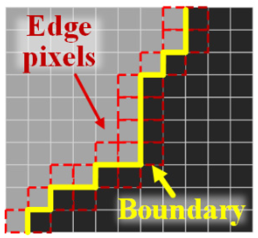
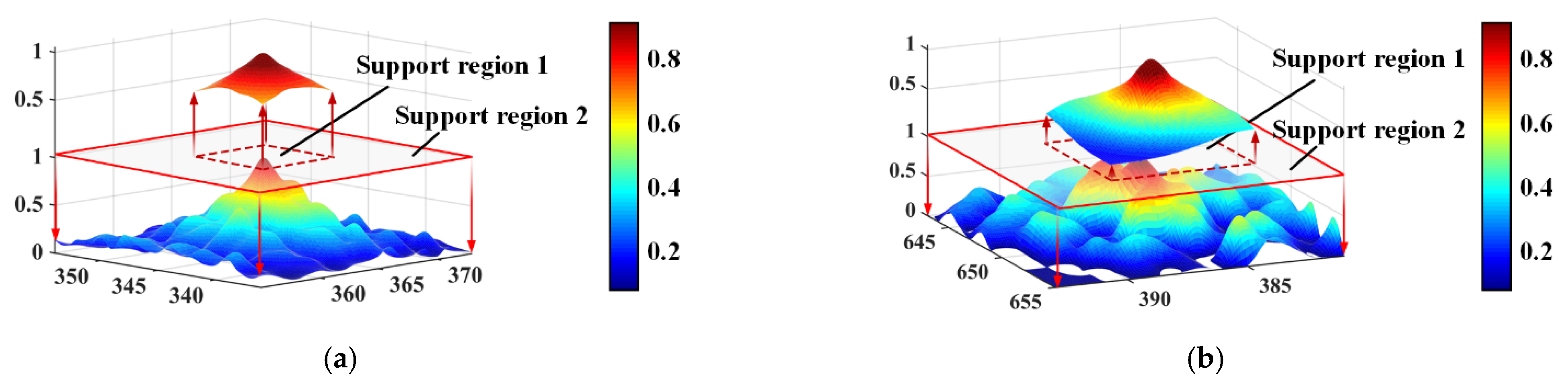
2.2.4. Guidance-Aided Edge Recovery Method

It was introduced in Section 2 that RGF’s framework provides a feature preservation method in the form of feedback. Nevertheless, the difference-based edge response in the RGF method leads to the high false alarm rate in SAR images. In this paper, the ratio of the exponentially weighted averages (ROEWA) method [30] is utilized to produce the guidance factor for edge recovery in a ratio-based way. It is worth mentioning that ROEWA is an optimal detector in the minimum mean square error sense, as is the Frost filter. The edge strength of ROEWA is

$$E^{\mathrm{ROEWA}}(p)=\sqrt{r_{X,\max }^2(p)+r_{Y,\max }^2(p)}$$

(12)

where $r_{X,\max }(p)$ and $r_{Y,\max }(p)$ are the horizontal and vertical edge strength components at $p$, respectively, and are defined as

$$\{\begin{array}{l}{r}_{X,\max }(p)=\max \left[{\mu }_{\mathbb{N}(p)}^{X-}/{\mu }_{\mathbb{N}(p)}^{X+},{\mu }_{\mathbb{N}(p)}^{X+}/{\mu }_{\mathbb{N}(p)}^{X-}\right]\\ r_{Y,\max }(p)=\max \left[{\mu }_{\mathbb{N}(p)}^{Y-}/{\mu }_{\mathbb{N}(p)}^{Y+},{\mu }_{\mathbb{N}(p)}^{Y+}/{\mu }_{\mathbb{N}(p)}^{Y-}\right]\end{array}$$

where ${\mu }_{region}^{direction}$ represents the exponential weighted average in the sub-region along the positive (+) or negative (−) direction of X- or Y-axis. For example, ${\mu }_{\mathbb{N}(p)}^{Y-}$ denotes the exponentially weighted average of the subregion along the negative direction of the Y-axis near $p$. The other parameters can be expressed in the same way.

Consequently, the guidance-aided Frost filter for SAR images is realized by introducing ratio-based edge response into original Frost, which can be expressed as

$$I^{\mathrm{GF}}(p)=\frac{1}{M_p^{\mathrm{G}}}{\displaystyle \sum _{q\in \mathbb{N}(p)}I(q)\cdot \exp \left(-\frac{\kappa {\Vert p-q\Vert }^2{C}_q^2}{2{\sigma }_s^2}-\frac{{\Vert E^{\mathrm{ROEWA}}(p)-E^{\mathrm{ROEWA}}(q)\Vert }^2}{2{\sigma }_r^2}\right)}$$

(13)

where $I^{\mathrm{GF}}$ represents the output of the guidance-aided Frost filter, and

$$M_p^{\mathrm{G}}={\displaystyle \sum _{q\in \mathbb{N}(p)}\exp \left(-\frac{\kappa {\Vert p-q\Vert }^2{C}_q^2}{2{\sigma }_s^2}-\frac{{\Vert E^{\mathrm{ROEWA}}(p)-E^{\mathrm{ROEWA}}(q)\Vert }^2}{2{\sigma }_r^2}\right)}.$$

It can be seen that the added factor, i.e., ${\Vert E^{\mathrm{ROEWA}}(p)-E^{\mathrm{ROEWA}}(q)\Vert }^2/2{\sigma }_r^2$, could reduce the filtering effect at the edges; the greater the edge strength, the greater the negative feedback to filtering.

2.2.5. Combination Version for All the Adaptiveness

Up to this point, the scale-adaptive neighborhood, the adaptive tuning factor, and the guidance-aided edge adaptive recovery were demonstrated. Therefore, the final proposed method is represented as follows:

$$I^{\mathrm{GTF}}(p)=\frac{1}{M_p^{\mathrm{TG}}}{\displaystyle \sum _{q\in {\mathbb{N}}_{\mathrm{sa}}(p)}I(q)\cdot \exp \left(-\frac{{\kappa }_{\mathrm{ad}}(q)\cdot {\Vert p-q\Vert }^2{C}_q^2}{2{\sigma }_s^2}-\frac{{\Vert E_{\mathrm{sa}}^{\mathrm{ROEWA}}(p)-E_{\mathrm{sa}}^{\mathrm{ROEWA}}(q)\Vert }^2}{2{\sigma }_r^2}\right)}$$

(14)

where

$$M_p^{\mathrm{TG}}={\displaystyle \sum _{q\in {\mathbb{N}}_{\mathrm{sa}}(p)}\exp \left(-\frac{{\kappa }_{\mathrm{ad}}(q)\cdot {\Vert p-q\Vert }^2{C}_q^2}{2{\sigma }_s^2}-\frac{{\Vert E_{\mathrm{sa}}^{\mathrm{ROEWA}}(p)-E_{\mathrm{sa}}^{\mathrm{ROEWA}}(q)\Vert }^2}{2{\sigma }_r^2}\right)}$$

(15)

$E_{\mathrm{sa}}^{\mathrm{ROEWA}}(p)$ denotes the edge response of ROEWA calculated in ${\mathbb{N}}_{\mathrm{sa}}(p)$. It is worth emphasizing that (14) also can be modified into an iterative version such as (6) if necessary. Although (14) seems a little complex, a simple implementation is shown in the pseudocode way, which is illustrated in Algorithm 1. According to the pseudocode, ones could find that the proposed guidance-aided triple-adaptive Frost filter requires no complex nesting or looping, but only needs to calculate the sliding window size map, edge response map, and adaptive tuning factor matrix sequentially and takes them into (14).

Algorithm 1 Guidance-aided triple-adaptive Frost filter.

Input: The original SAR image $I$, iteration times $n$, ${\sigma }_s$, ${\sigma }_r$, $d_{\min }$, $d_{\max }$. Output: The filtered image $I_{\mathrm{out}}$ Initialize: $i=1$. Begin 1: $I_0=I$ 2:   for $i\le n$ do 3:      Obtain the scale-adaptive sliding window size map $S(I_0)$ of image $I_i$; 4:      Obtain the edge response map ${\mathit{E}}_{\mathrm{sa}}^{\mathrm{ROEWA}}$ of image $I_i$ referring to $S\left(I_0\right)$; 5:      Calculate the adaptive tuning factor matrix ${\kappa }_{\mathrm{ad}}$; 6:      Generate the filtered image $I_{i+1}$ by taking $S\left(I_0\right)$, ${\mathit{E}}_{\mathrm{sa}}^{\mathrm{ROEWA}}$, and ${\kappa }_{\mathrm{ad}}$ into (14); 7:     $i=i+1$; 8:   end; 9:   The output image $I_{\mathrm{out}}=I_n$; End.

3. Experiments

3.1. Experimental Design

In this paper, the scale-adaptive sliding window sizing method, adaptive tuning factor, and guidance-aided adaptive edge recovery method are introduced for the final proposed filter. Therefore, it is necessary to verify their performances in the proper ways, which are detailed in this Section.

For the scale-adaptive sliding window sizing method, the accuracy of edge positioning and the responsiveness of the sizing algorithm are significant. Both of them are influenced by the distance between two adjacent edges, i.e., the width of homogeneous region and the contrast at the edge. Therefore, we manually draw two simulated textured images, as Figure 6 shows, to test the performance of the scale-adaptive sliding window sizing method. There are 40 uniform stripes contained in Figure 6a, whose widths gradually and uniformly decrease from 100 pixels to 5 pixels. The pixel intensity in light regions is set as 150, and that of the dark regions is 50. It can be seen that the narrower the width of the stripes, the stricter the requirements for our sliding window sizing method. Similarly, there are 40 stripes in Figure 6b. Nevertheless, all their widths are fixed as 52 pixels, but the intensity differences between two adjacent stripes change from 160 to 8 diminishingly. It can be used to effectively verify the responsiveness of the method. Both images in Figure 6 are polluted by speckle noise with a standard deviation of 0.05.

For the guidance-aided edge recovery factor and adaptive tuning factor combined with the scale-adaptive neighborhood, their performance can be verified by comparing the local weight template $W$ based on a fixed tuning factor (as the way in original Frost method) and the locally weighted template $W^{\mathrm{TG}}$ based on (11) and (8), which can be written as

$$W(q)=\frac{1}{M_p}\cdot \exp \left(-\kappa {\Vert p-q\Vert }^2{C}_q^2\right), \mathrm{s}.\mathrm{t}. q\in \mathbb{N}(p)$$

and

$$\{\begin{array}{l}{W}^{\mathrm{TG}}(q)=\frac{1}{M_p^{\mathrm{TG}}}\cdot \exp \left(-\frac{{\kappa }_{\mathrm{ad}}(q)\cdot {\Vert p-q\Vert }^2{C}_q^2}{2{\sigma }_s^2}-\frac{{\Vert E_{\mathrm{sa}}^{\mathrm{ROEWA}}(p)-E_{\mathrm{sa}}^{\mathrm{ROEWA}}(q)\Vert }^2}{2{\sigma }_r^2}\right), \mathrm{s}.\mathrm{t}. q\in {\mathbb{N}}_{\mathrm{sa}}(p)\\ {\kappa }_{\mathrm{ad}}(q)=T(p)\cdot Q(q)\\ Q(q)=\frac{\left|I(q)-I(p)\right|}{\frac{1}{{\mathbb{N}}_{\mathrm{sa}}(p)-1}{\displaystyle \sum _{q\in {\mathbb{N}}_{\mathrm{sa}}(p)}\left|I(q)-I(p)\right|}}\end{array}$$

Furthermore, verification of the filtering performance of the proposed is essential. We gather both the synthetic images and natural single-polarization airborne SAR images, as Figure 7 shows, in order to test the effect of our method. All the natural SAR images are supported by the Aerospace Information Research Institute, Chinese Academy of Sciences. The parameter settings of the proposed guidance-aided triple-adaptive Frost filter are illustrated in

Table 1. Sizes and parameter sets of the proposed method for images.

Image	Size	$\mathbf{Parameter} \mathbf{Set} (\mathit{n}, {\mathit{\sigma }}_{\mathit{s}}, {\mathit{\sigma }}_{\mathit{r}}, {\mathit{d}}_{\mathbf{min}}, {\mathit{d}}_{\mathbf{max}})$
Synthetic image	880 × 880	(1, 10, 0.05, 7, 19)
Plant	300 × 300	(1, 50, 0.05, 5, 13)
Clamps	300 × 300	(1, 3, 0.05, 5, 13)
Keyboard	300 × 300	(1, 50, 0.05, 5, 13)
apple	300 × 300	(1, 80, 0.05, 5, 13)
Ku-band SAR image	2224 × 1668	(1, 50, 0.1, 9, 25)
S-band SAR image	5460 × 3580	(1, 50, 0.1, 11, 31)

.

3.2. Experimental Results

In this section, the experiment results for the performance of the scale-adaptive sliding window sizing method and guidance-aided adaptive weight template in (14) are demonstrated first, and then we discuss the speckle suppression experimental results on three images in Figure 7, in terms of multiple metrics of the filtered images in different methods.

3.2.1. The Performance of Scale-Adaptive Sliding Window Sizing Method

As aforementioned, there are two synthetic textured and speckled images illustrated in Figure 6. We set $(d_{\min },d_{\max })=(7,19)$ arbitrarily for all the tests in this part. The positioning accuracy of the scale-adaptive sliding window sizing method can be verified with the first image, in which the stripe widths are gradually narrowing, resulting in the difficulty of the edge positioning increasing. Thus, its response result is demonstrated in Figure 8, where the curve in lavender represents pixel intensity and the pink curve is the size of the sliding window. It can be found that the size of the adaptive sliding window is able to decrease near the edges and increase away from them, even though the speckle noise causes drastic pixel intensity fluctuations in the uniform regions. As the reason that the widths of the stripes at the right in Figure 8 are too narrow to make sliding window size increase to the maximum, the pink curve for window size seems to be unstable, but in fact it is reasonable.

The sensitivity of the response refers to the accuracy of the size-adaptive sliding window method in detecting edges with different contrasts. There are stripes with decreasing intensity differences shown in Figure 6b, which can be used to test the sensitivity of the response. Accordingly, the experimental result is shown in Figure 9. Different from the result in Figure 8, the scale-adaptive sliding window sizing method fails to distinguish the edges at the right. That is because the pixel intensity fluctuations, resulting from speckle noise, lead to stripes mixing together. Thus, the scale-adaptive sliding window sizing method regards these regions as homogeneous. Although it is explainable, the finite response sensitivity is still confirmed.

3.2.2. The Performance of Guidance-Aided Adaptive Weighting Template

Traditional Frost filter uses the fixed tuning factor for speckle suppression, which means that it is difficult to take into account the specific situation for various regions in the image. Therefore, the adaptive tuning factor as (11) makes it is possible to adjust itself in a fixed neighborhood range. However, the size of the support region affects the samples to gather statistical data, which is important for (11). As mentioned in Section 3, different kinds of tuning factor influence the weighting template of the Frost filter. We select two points randomly in Figure 1a to demonstrate the weighting template intuitively, and the results are presented in Figure 10. The coordinates of the two selected points are (364, 345), which is in the uniform region, and (387, 649) at the edge. The traditional weighting templates are placed on top, and the novel weighting templates of our method are placed on the bottom. The squares boxed in a red line represent the scale-adaptive support regions, while the squares dotted in red indicate the original support regions. In Figure 10, to make the templates smooth enough, all of them are interpolated by bicubic interpolation processing.

According to Figure 10, the support regions (i.e., support region 2) resulting from our method are different for two points. While it is in the homogeneous region, the guidance-aided adaptive weighting template, which is Gaussian-like, covers a large range, and the template assigns more weight to the regions near the center. As for the traditional weighting template in Figure 10a, whose support region (i.e., support region 1) is fixed as 7 × 7, all pixels in it are assigned larger weights. When the central point is at the edge, the traditional weighting template only makes pixels near the center gain more weight, but it does not seem to reflect any consideration on the edge location in the support region. On the contrary, our method not only shrinks the support region compared to Figure 10a, but also distributes the weights strategically at different locations within the support region.

In general, the weighting template in our method can dynamically adjust the weight template according to the position where it is and assign the weights more reasonably.

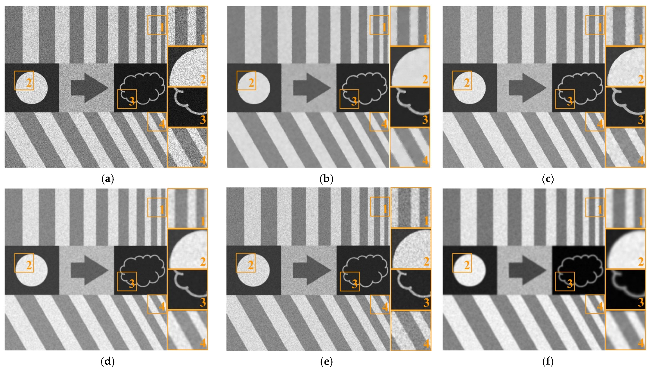
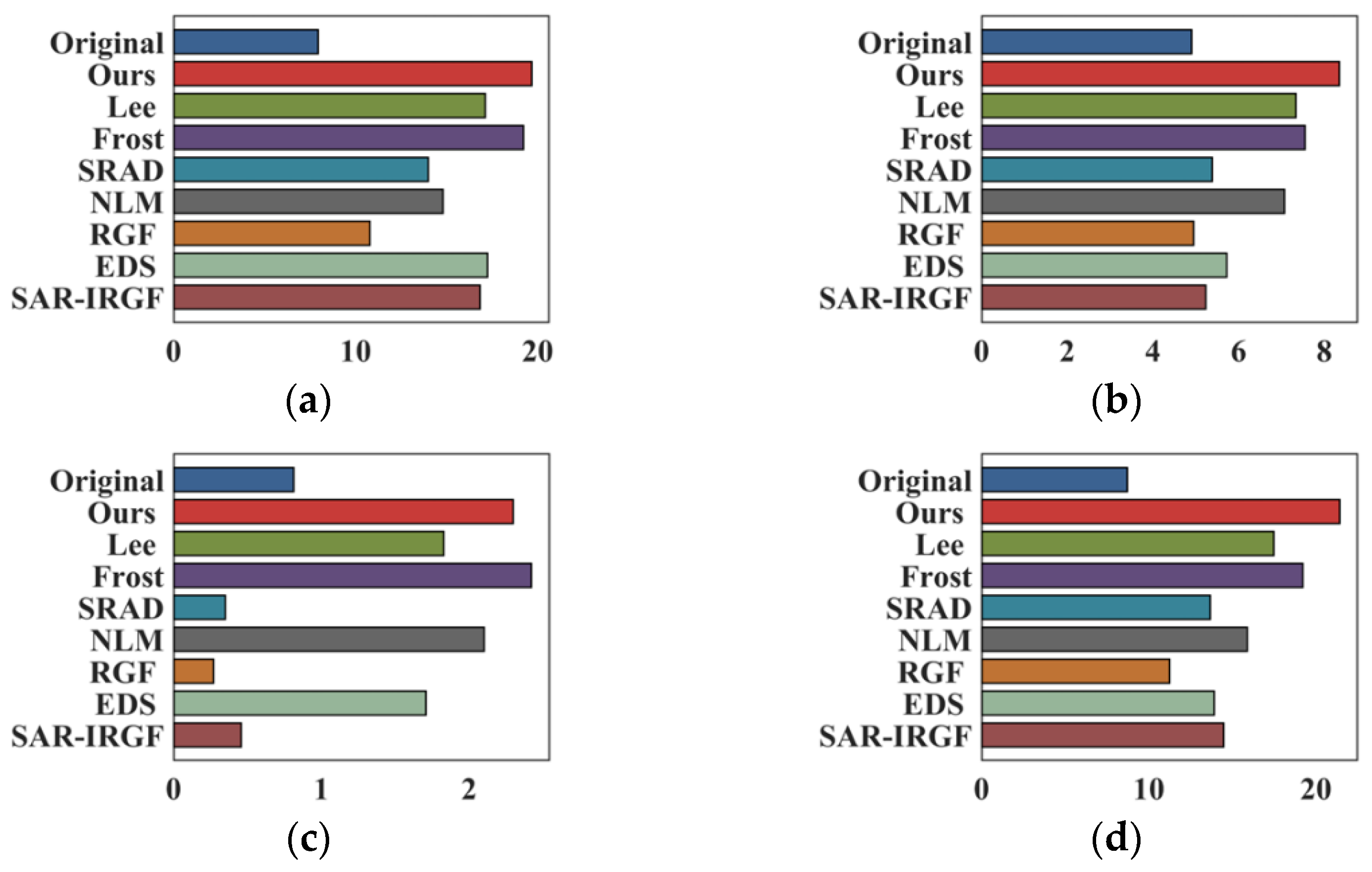
3.2.3. Experimental Results for Speckle Suppression on the Synthetic Images

Firstly, on the one hand, the speckle noise with a standard deviation 0.05 is added to the synthetic image, which is shown in Figure 7a. On the other hand, as comparison methods, Lee filter, traditional Frost filter, SRAD method, NLM method, RGF method, enhanced directional smoothing (EDS) [31], and SAR-IRGF are used to denoise this image with the proposed method in this paper. The detailed parameter setting for our method is recorded in Table 1, and the parameter settings for other methods are determined according to the recommendations of their respective authors. Then, the speckle suppression results are illustrated in Figure 11. Moreover, four different kinds of regional parts in the synthetic image are boxed in orange. There are vertical stripes, dividing lines between homogeneous regions, narrow edges, and angled stripes in them, respectively.

It can be found that most speckle suppression methods blur edges except for ours, the Lee filter, NLM filter, and RGF method. There are still obvious residual flare-like things left in the uniform regions in Figure 11c,f, due to the incomplete smoothing. The NLM method produces many regular, fine textures, which is attributed to its patch-based mechanism. Objectively, we utilize the equivalent number of looks (ENL) [32], edge preservation index (EPI) [33], and structural similarity index measure (SSIM) [34] to evaluate the speckle suppression performance of each method. These indicators are recorded in Figure 12, Figure 13 and Figure 14. Based on these indicators, ones can find that the proposed method is the most thorough in speckle suppression, and keeps the most similar structure to the original image.

Next, four optical images are utilized to test the performance of our method in real-world scenes. Note that, due to many features existing in the plant, the clamps, and the keyboard, we add less speckle with a standard deviation of 0.03 on them. The speckle with a standard deviation 0.06 pollutes the Apple, in order to verify the methods’ filtering ability. The filtering results are presented in Figure 15. According to Figure 15, one could easily find that our method protects features better visually while speckle is removed, especially the preserved letters on the keyboard for example. Furthermore, the comparisons of ENL, EPI, and SSIM for all the results in Figure 15 are illustrated in Figure 16. Based on Figure 16, one could find that the proposed method performs best speckle suppression in most cases with satisfying feature preservation.

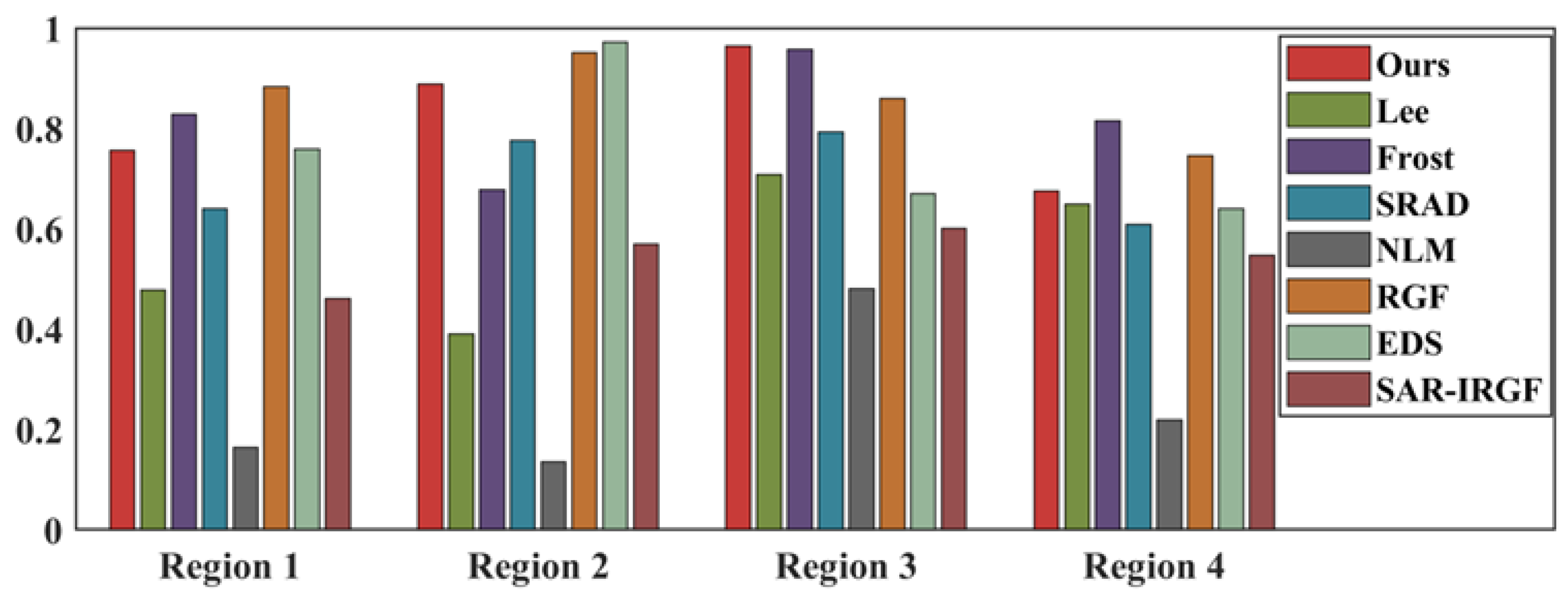
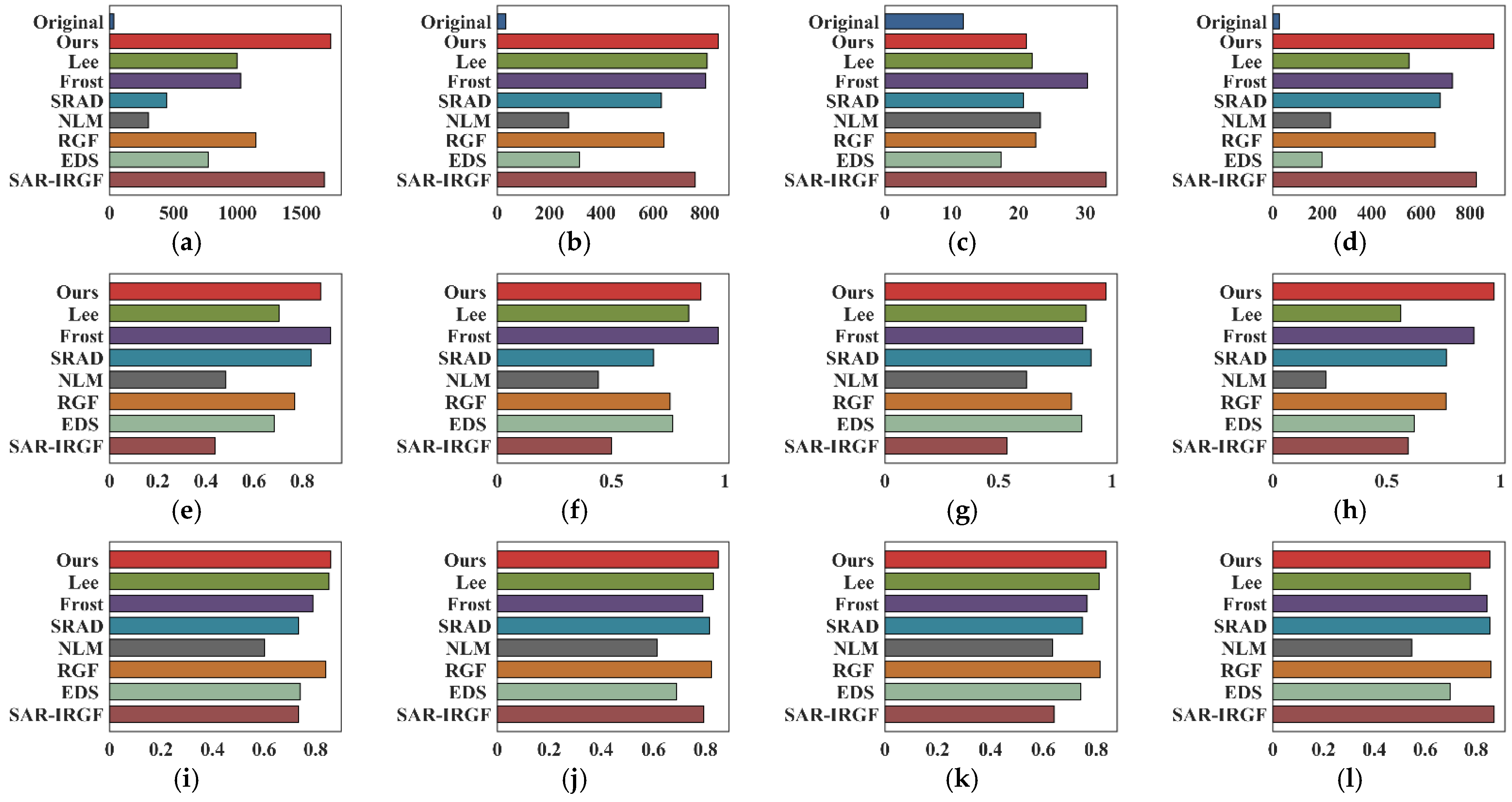
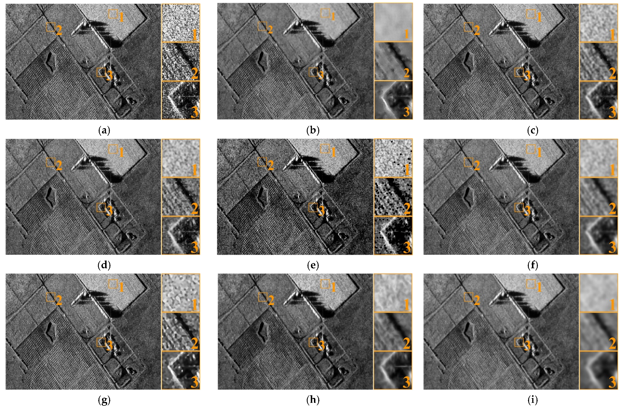
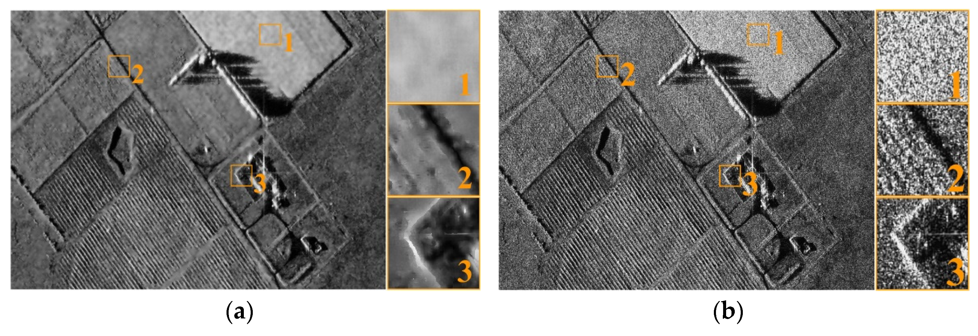
3.2.4. Experimental Results for Speckle Suppression on the Airborne SAR Images

There are two natural airborne SAR images to test the filtering performance of different methods. The first one is Ku-band, and contains a lot of crops arranged in a regular pattern in the farmland, which can be found on the bottom of the image, and a little building is located near subregion 3. Therefore, it is naturally desirable for the speckle suppression methods to smooth out as much as possible the noise in uniform regions in the farmland and to preserve the feature of aforementioned crops, while retaining the sharp boundaries of farmlands and the building. According to the filtered results in Figure 17, the Lee filter, Frost filter, RGF method, and EDS method fail to blur the homogeneous regions, such as subregion 1. There is new noise mixed into the filtering result of the patch-based method, whose reason is its poor scale adaptivity during the patch search. Our method seems to perform best. However, it is not objective to make the conclusion visually only according to the image results. Hence, we calculate the ENL of three subregions in Figure 17, and place the comparison of ENL values in Figure 18. Note that the EPI and SSIM are reference-based indicators, which means they cannot be obtained for the experimental results on a natural SAR image due to the lack of noiseless original image for reference. It can be seen that our method makes ideal ENL results in the uniform regions, and filters less in the region where edges are located.

As for the S-band airborne SAR image as Figure 7c, it corresponds to a very large area in the ground, from which many agricultural fields can be seen neatly arranged. There are also many houses distributed among farmlands. It is challenging for the de-speckling methods to preserve the clear farmland boundaries in this image. Correspondingly, the filtering results of all methods are shown in Figure 19. In fact, the aforementioned newly introduced noise is still present in Figure 19f, which is filtered by the NLM method. However, it is difficult to see this phenomenon in the image because of the large size of the S-band SAR image. The ENL value comparison results calculated from four selected regions are illustrated in Figure 20. It can be found that the proposed method performs well in subregion 1, subregion 2, and subregion 4, benefiting from the boundaries with large contrast there. Nevertheless, there are tiny edges in subregion 3, which are almost filtered out by our method and SAR-IRGF method. That is owed to the insensitivity of our method to the weak contrast edges, as demonstrated by the result in Figure 9. On the other hand, the proposed guidance-aided triple-adaptive Frost filter achieves best ENL results, according to Figure 20.

4. Discussion

The speckle is a multiplicative noise existing in SAR images and medical ultrasound images. Its destructiveness is reflected in the different noise fluctuations caused to regions with various scattering intensities, which leads to the demand for spatial domain speckle suppression algorithms to have the distinguishability between categories of regions. In this paper, triple adaptiveness is bestowed on the traditional Frost filter, i.e., the adaptabilities for neighborhood sizing, tuning factor, and feature preservation. The improved Frost filter is as (14), in which ${\mathbb{N}}_{\mathrm{sa}}$ denotes the scale-adaptive neighborhood, ${\kappa }_{\mathrm{ad}}$ is adaptive tuning factor according to (11), and ${\Vert E^{\mathrm{ROEWA}}(p)-E^{\mathrm{ROEWA}}(q)\Vert }^2/2{\sigma }_r^2$ represents the adaptive feature recovery factor. Referring to Figure 8 and Figure 9, the positioning accuracy and contrast sensitivity of ${\mathbb{N}}_{\mathrm{sa}}$ can be verified. The comparisons between the performances of novel filtering weight template and the original are demonstrated in Figure 10, from which it can be found both the sizes of templates and weight values change with position. In particular, the sliding window size is 18 × 18, as Figure 10a shows, while it is in the uniform region, and its size shrinks to 12 × 12, while the central pixel is near the edge. Furthermore, the weight assignment also behaves differently. The filtering results of experiments on images in Figure 7 show the superiority of our methods. The most obvious one is the good protection for sharp edges. It is important to know that the traditional Frost filter was criticized for its unsatisfactory edge protection before this. Although all the iteration numbers for our method are set as 1, it supports to be implemented in an iterative way, which can be referred to (6), and in our previous work [24], there is evidence that the ROEWA-guided RGF filtering method has better convergence.

From Algorithm 1, one can realize that the proposed method is very easy to implement. Therefore, it is feasible to apply our method to some real-time processing platform, such as the field programmable gate array, the digital signal processor, etc. Although it was previously mentioned that ML-based denoising methods are not suitable for real-time applications and they are not the focus of this paper for comparison. We still illustrate the de-speckling performance of the denoising convolutional neural network (DnCNN) [12], which is well trained. The filtered result of the aforementioned Ku-band SAR image by DnCNN is presented in Figure 21b. As a contrast, the suppression result of our method is placed next to it. Obviously, DnCNN fails to remove the speckle noise effectively from the SAR image. The ENLs of the three subregions in the filtering result of the DnCNN method are 7.602, 2.264, and 1.469, respectively. In contrast, those of the corresponding regions from the proposed method reach 549.524, 9.527, and 3.196.

5. Conclusions

In this paper, a novel guidance-aided triple-adaptive Frost filter is proposed for speckle suppression in the SAR image. The scale-adaptive sliding window sizing method, which can resize a neighborhood for various points, is used to determine the support region for subsequent image processing. Next, the adaptive tuning factor and the guidance information for edge recovery are adopted in our method. Although multiple adaptive technologies are applied into our method, it is still easy to implement, even for the real-time processing platform. Both the positioning accuracy and response sensitivity are verified by experimental results. Speckle suppression experiment results on the synthetic image and two natural airborne SAR images verify the superiority of the proposed method in comparison with other de-speckling methods.

Further, on the one hand, we will test the performance of the proposed method on a larger dataset and apply it into other remote sensing applications. On the other hand, scale-adaptive technology will be further explored.

References

1. Liang, J.; Liu, X.; Huang, K.; Li, X.; Wang, D.; Wang, X. Automatic Registration of Multisensor Images Using an Integrated Spatial and Mutual Information (SMI) Metric. IEEE Trans. Geosci. Remote Sens. 2014, 52, 603–615. [Google Scholar] [CrossRef]
2. Chang, H.H.; Chan, W.C. Automatic Registration of Remote Sensing Images Based on Revised SIFT With Trilateral Computation and Homogeneity Enforcement. IEEE Trans. Geosci. Remote Sens. 2021, 59, 7635–7650. [Google Scholar] [CrossRef]
3. Zhang, J.; Wu, L.; Lin, G.; Cheng, Y. An Integrated De-Speckling Approach for Medical Ultrasound Images Based on Wavelet and Trilateral Filter. Circuits Syst. Signal Process. 2016, 36, 297–314. [Google Scholar] [CrossRef]
4. Li, J.; Wang, Z.; Yu, W.; Luo, Y.; Yu, Z. A Novel Speckle Suppression Method with Quantitative Combination of Total Variation and Anisotropic Diffusion PDE Model. Remote Sens. 2022, 14, 796. [Google Scholar] [CrossRef]
5. May, V.; Keller, Y.; Sharon, N.; Shkolnisky, Y. An Algorithm for Improving Non-Local Means Operators via Low-Rank Approximation. IEEE Trans. Image Process. 2016, 25, 1340–1353. [Google Scholar] [CrossRef] [Green Version]
6. Deledalle, C.A.; Denis, L.; Tupin, F. Iterative Weighted Maximum Likelihood Denoising with Probabilistic Patch-Based Weights. IEEE Trans. Image Process. 2009, 18, 2661–2672. [Google Scholar] [CrossRef] [Green Version]
7. Rudin, L.I.; Osher, S.; Fatemi, E. Nonlinear Total Variation Based Noise Removal Algorithms. Phys. D 1992, 60, 259–268. [Google Scholar] [CrossRef]
8. Perona, P.; Malik, J. Scale-Space and Edge Detection Using Anisotropic Diffusion. IEEE Trans. Pattern Anal. Mach. Intell. 1990, 12, 629–639. [Google Scholar] [CrossRef] [Green Version]
9. Yu, Y.; Acton, S.T. Edge Detection in Ultrasound Imagery Using the Instantaneous Coefficient of Variation. IEEE Trans. Image Process. 2004, 13, 1640–1655. [Google Scholar] [CrossRef]
10. Yu, Y.; Acton, S.T. Speckle Reducing Anisotropic Diffusion. IEEE Trans. Image Process. 2002, 11, 1260–1270. [Google Scholar] [CrossRef]
11. Gu, S.; Zhang, L.; Zuo, W.; Feng, X. Weighted Nuclear Norm Minimization with Application to Image Denoising. In Proceedings of the IEEE Computer Society Conference on Computer Vision and Pattern Recognition, Columbus, OH, USA, 23–28 June 2014; pp. 2862–2869. [Google Scholar] [CrossRef] [Green Version]
12. Simonyan, K.; Zisserman, A. Very Deep Convolutional Networks for Large-Scale Image Recognition. arXiv 2014, arXiv:1409.1556. [Google Scholar]
13. Chen, Q.; Montesinos, P.; Sen, Q.; Xia, D.S. Ramp Preserving Perona—Malik Model. Signal Process. 2010, 90, 1963–1975. [Google Scholar] [CrossRef]
14. Lin, H.; Zhuang, Y.; Huang, Y.; Ding, X. Self-Supervised SAR Despeckling Powered by Implicit Deep Denoiser Prior. IEEE Geosci. Remote Sens. Lett. 2022, 19, 3212078. [Google Scholar] [CrossRef]
15. Dalsasso, E.; Denis, L.; Tupin, F. SAR2SAR: A Semi-Supervised Despeckling Algorithm for SAR Images. IEEE J. Sel. Top. Appl. Earth Obs. Remote Sens. 2021, 14, 4321–4329. [Google Scholar] [CrossRef]
16. Ma, Y.; Suda, N.; Cao, Y.; Vrudhula, S.; Seo, J. sun ALAMO: FPGA Acceleration of Deep Learning Algorithms with a Modularized RTL Compiler. Integration 2018, 62, 14–23. [Google Scholar] [CrossRef]
17. Frost, V.S.; Abbott Stiles, J.; Shanmugan, K.S.; Holtzman, J.C. A Model for Radar Images and Its Application to Adaptive Digital Filtering of Multiplicative Noise. IEEE Trans. Pattern Anal. Mach. Intell. 1982, PAMI-4, 157–166. [Google Scholar] [CrossRef]
18. Lindeberg, T. Scale-Space: A Framework for Handling Image Structures at Multiple Scales. In Proceedings of the CERN School of Computing, Egmond aan Zee, The Netherlands, 8–21 September 1996. [Google Scholar]
19. Koenderink, J.J. The Structure of Images. Biol. Cybern. 1984, 50, 363–370. [Google Scholar] [CrossRef]
20. Lindeberg, T. Scale-Space Theory: A Basic Tool for Analysing Structures at Different Scales. J. Appl. Stat. 1994, 21, 224–270. [Google Scholar] [CrossRef] [Green Version]
21. Lindeberg, T. Scale-Space Theory in Computer Vision; Springer: New York, NY, USA, 1994. [Google Scholar]
22. Zhang, Q.; Shen, X.; Xu, L.; Jia, J. Rolling Guidance Filter. In Proceedings of the European Conference on Computer Vision 2014, Zurich, Switzerland, 6–12 September 2014; Springer: Cham, Switzerland, 2014. [Google Scholar]
23. Jing, W.-B.; Jin, T.; Xiang, D.-L. Edge-Aware Superpixel Generation for SAR Imagery With One Iteration Merging. IEEE Geosci. Remote Sens. Lett. 2021, 18, 1600–1604. [Google Scholar] [CrossRef]
24. Li, J.; Wang, Z.; Yu, W.; Yu, Z. SAR-IRGF: A Novel Improved Rolling Guidance Filter for the Synthetic Aperture Radar Image. Electron. Lett. 2022, 58, 828–830. [Google Scholar] [CrossRef]
25. Chen, J.; Chen, S.; Liu, Y.; Chen, X.; Yang, Y.; Zhang, Y. Robust Local Structure Visualization for Remote Sensing Image Registration. IEEE J. Sel. Top. Appl. Earth Obs. Remote Sens. 2021, 14, 1895–1908. [Google Scholar] [CrossRef]
26. Guo, Q.; Wang, H.; Member, S.; Kang, L.; Li, Z.; Xu, F. Aircraft Target Detection from Spaceborne SAR Image. In Proceedings of the IGARSS 2019—2019 IEEE International Geoscience and Remote Sensing Symposium, Yokohama, Japan, 28 July–2 August 2019; IEEE: Piscataway, NJ, USA, 2019; pp. 1168–1171. [Google Scholar]
27. Chen, L.; Jiang, X.; Li, Z.; Liu, X.; Zhou, Z. Feature-Enhanced Speckle Reduction via Low-Rank and Space-Angle Continuity for Circular SAR Target Recognition. IEEE Trans. Geosci. Remote Sens. 2020, 58, 7734–7752. [Google Scholar] [CrossRef]
28. Hui-Zhen, J.; Wang, T.-H. Modified Frost Filtering Based on Adaptive Parameter. Comput. Eng. Des. 2011, 32, 3793–3843. [Google Scholar] [CrossRef]
29. Sun, Z.; Zhang, Z.; Chen, Y.; Liu, S.; Song, Y. Frost Filtering Algorithm of SAR Images with Adaptive Windowing and Adaptive Tuning Factor. IEEE Geosci. Remote Sens. Lett. 2020, 17, 1097–1101. [Google Scholar] [CrossRef]
30. Fjørtoft, R.; Lopes, A.; Cubero-Castan, E. An Optimal Multiedge Detector for SAR Image Segmentation. IEEE Trans. Geosci. Remote Sens. 1998, 36, 793–802. [Google Scholar] [CrossRef] [Green Version]
31. Mastriani, M.; Giraldez, A.E. Enhanced Directional Smoothing Algorithm for Edge-Preserving Smoothing of Synthetic-Aperture Radar Images. Meas. Sci. Rev. 2014, 4, 1–11. [Google Scholar] [CrossRef]
32. Anfinsen, S.N.; Doulgeris, A.P.; Eltoft, T. Estimation of the Equivalent Number of Looks in Polarimetric Sar Imagery. In Proceedings of the International Geoscience and Remote Sensing Symposium (IGARSS), Boston, MA, USA, 7–11 July 2008; IEEE: Piscataway, NJ, USA, 2008; Volume 4, pp. 487–490. [Google Scholar]
33. Kuppusamy, P.G.; Joseph, J.; Sivaraman, J. A Full Reference Morphological Edge Similarity Index to Account Processing Induced Edge Artefacts in Magnetic Resonance Images. Biocybern. Biomed. Eng. 2017, 37, 159–166. [Google Scholar] [CrossRef]
34. Huang, Y.; Xia, W.; Lu, Z.; Liu, Y.; Chen, H.; Zhou, J.; Fang, L.; Zhang, Y. Noise-Powered Disentangled Representation for Unsupervised Speckle Reduction of Optical Coherence Tomography Images. IEEE Trans. Med. Imaging 2021, 40, 2600–2614. [Google Scholar] [CrossRef]
Figure 1. Three examples for presentation of the speckle noise; (a) is a synthetic speckled image; and (b,c) are two Ku-band airborne SAR images containing various targets.
Remotesensing 15 00551 g001
Figure 2. Schematic diagram for the anisotropic diffusion.
Remotesensing 15 00551 g002
Figure 3. Gaussian scale space.
Remotesensing 15 00551 g003
Figure 4. Schematic for the edge in the discrete image.
Remotesensing 15 00551 g004
Figure 5. The simulated performance of the scale-adaptive neighborhood.
Remotesensing 15 00551 g005
Figure 6. The synthetic images for verifying the performance of the scale-adaptive sliding window sizing method; (a) is a synthetic textured image for the positioning accuracy experiment; and (b) is a synthetic textured image for the response sensitivity experiment.
Remotesensing 15 00551 g006
Figure 7. The images for speckle suppression experiments: (a) is a computer-generated synthetic image; (be) are camera pictures for a plant, five clamps, a keyboard, and an apple, respectively; (f) is an original single-look Ku band airborne SAR image captured in October 2020; and (g) is another original single-look S-band airborne SAR image captured in April 2022.
Remotesensing 15 00551 g007
Figure 8. The experimental result for edge positioning accuracy.
Remotesensing 15 00551 g008
Figure 9. The experimental result for response sensitivity.
Remotesensing 15 00551 g009
Figure 10. Comparison for the traditional weighting template and the guidance-aided adaptive weighting factor in the Frost filter: (a) is the comparison for the weight template in uniform region; (b) is the comparison for the weight template near the edge. The dotted squares represent the support regions of the traditional Frost filter, and the red squares are support regions of the proposed method.
Remotesensing 15 00551 g010
Figure 11. Experimental results on the synthetic image: (a) is the original image, and (bi) are filtered results of our method, Lee filter, traditional Frost filter, SRAD, NLM, RGF, EDS, and SAR-IRGF.
Remotesensing 15 00551 g011aRemotesensing 15 00551 g011b
Figure 12. ENL results for the regional parts of speckle suppression images: (ad) are the ENL results of subregion 1, subregion 2, subregion 3, and subregion 4, respectively, in the synthetic image.
Remotesensing 15 00551 g012
Figure 13. EPI results for the speckle suppression on synthetic image.
Remotesensing 15 00551 g013
Figure 14. SSIM results for the speckle suppression on synthetic image.
Remotesensing 15 00551 g014
Figure 15. Experimental results of four optical images: (a18) are the denoising results for the Plant of our method, Lee filter, traditional Frost filter, SRAD, NLM, RGF, EDS, and SAR-IRGF, respectively. (b18) are the denoising results for the Clamps of our method, Lee filter, traditional Frost filter, SRAD, NLM, RGF, EDS, and SAR-IRGF, respectively. (c18) are the denoising results for the Keyboard of our method, Lee filter, traditional Frost filter, SRAD, NLM, RGF, EDS, and SAR-IRGF, respectively. (d18) are the denoising results for the Apple of our method, Lee filter, traditional Frost filter, SRAD, NLM, RGF, EDS, and SAR-IRGF, respectively.
Remotesensing 15 00551 g015
Figure 16. ENL, EPI, and SSIM results for the speckle suppression on four optical images: (ad) are the ENL comparison results for the plant, clamps, the keyboard, and the apple, respectively. Similarly, (eh) are their corresponding EPI results, while (il) are their SSIM results.
Remotesensing 15 00551 g016
Figure 17. Experimental results on the Ku-band SAR image: (a) is the original image, and (bi) are filtered results of our method, Lee filter, traditional Frost filter, SRAD, NLM, RGF, EDS, and SAR-IRGF, respectively.
Remotesensing 15 00551 g017
Figure 18. ENL results for the speckle suppression on Ku-band SAR image: (ac) are the ENL results corresponding to subregion 1 to 3, respectively.
Remotesensing 15 00551 g018
Figure 19. Experimental results on the S-band SAR image: (a) is the original image, and (bi) are filtered results of our method, Lee filter, traditional Frost filter, SRAD, NLM, RGF, EDS, and SAR-IRGF, respectively.
Remotesensing 15 00551 g019
Figure 20. ENL results for the regional parts of speckle suppression images: (ad) are the ENL results corresponding to subregion 1 to 4, respectively.
Remotesensing 15 00551 g020
Figure 21. Comparison of the de-speckling results between the proposed method and the DnCNN method: (a,b) are filtering results of our method and the DnCNN method, respectively.
Remotesensing 15 00551 g021