Abstract
Understanding the hydrological surface condition changes, climate change and their combined impacts on flood runoff are critical for comprehending the hydrology under environmental changes and for solving future flood management challenges. This study was designed to examine the relative contributions of the hydrological surface condition changes and climate change in the flood runoff of a 45,421-km2 watershed in the Loess Plateau region. Statistical analytical methods, including Kendall’s trend test, the Theisen median trend analysis, and cumulative anomaly method, were used to detect trends in the relationship between the climatic variables, the normalized difference vegetation index (NDVI), land use/cover change (LUCC) data, and observed flood runoff. A grid-cell distributed rainfall–runoff model was used to detect the quantitative hydrologic responses to the climatic variability and land-use change. We found that climatic variables were not statistically significantly different (p > 0.05) over the study period. From 1985 to 2013, the cropland area continued to decrease, while the forest land, pastures, and residential areas increased in the Jinghe River Basin. Affected by LUCC and climate change, the peak discharges and flood volumes decreased by 8–22% and 5–67%, respectively. This study can provide a reference for future land-use planning and flood runoff control policy formulation and for revision in the study area.
1. Introduction
In recent years, the global water cycle system has undergone tremendous changes due to the comprehensive action of the external environment (such as climate change and human activity interference) [1,2]. The hydrological system is affected by changes in the external environment, resulting in significant changes in water resources’ spatial and temporal distribution. More countries and regions face many water problems [3,4,5]. Runoff, an essential link in the hydrological cycle and the primary source of floods, is closely related to climate change and human activity interference [6,7,8]. Human activity interference is an important cause of land use/cover change (LUCC), which is one of the important indicators of hydrological surface condition changes [9,10,11]. LUCC is an important factor affecting regional hydrological characteristics [12,13]. LUCC can lead to changes in the hydrological processes and water distribution patterns, such as runoff, infiltration, and lateral flow [14,15].
The Loess Plateau is in the dryland region of Northwest China. It has an altitude of 800–3000 m and an area of 620,000 km2. It is one of the most water-scarce regions in China [16,17,18]. It also has thousands of gullies and ravines, that are more than 80% dry, yet frequently troubled by flash floods and mountain torrents during rainstorms [19]. Due to its unique geographical environment, insufficient natural water resources, and fragile ecological environment, the hydrology and ecosystem of the Loess Plateau are sensitive to climate change, hydrological surface condition changes, and other external environmental changes [20]. LUCC has a significant impact on environmental sustainability [21]. The evolution of the hydrology and ecosystem has a strong uncertainty and complexity [22]. The mechanism of watershed runoff evolution, driven by external environmental changes in the Loess Plateau has become a challenging issue for global scholars [23].
Many scholars have adopted hydrological model methods to study the mechanism of runoff evolution under changing environments [24,25,26,27,28,29,30]. For instance, Wang et al. [31] established a distributed time-varying gain model in the Chaobai River, that simulated and analyzed the monthly runoff changes. They deduced that climate change and human activity interference contributed 32% and 68% to runoff change, respectively. Hu et al. [32] used the climate elasticity and the M–K trend test method to quantitatively analyze the runoff response of the Gushanchuan watershed under a changing environment. Their results showed 12.9–15.1% and 84.9–87.1% climate change and LUCC contributions, respectively. Elsewhere, Guo et al. [33] used the hydrological statistical model and the distributed hydrological model (GBHM) to simulate and analyze the response variation status of the hydrological variables in the Chabagou watershed of the Loess Plateau in Northern Shaanxi, and attributed them to climate change, as well as to soil and water conservation. They thought that the hydrological process of the Loess Plateau watershed was mainly affected by human activities, and the attribution analysis results were relatively uncertain. Guo et al. [34] established the SWAT model for the Chaohe River Basin. They analyzed the impact of climate change and LUCC on runoff in the Basin, and quantified the runoff response of the Chaohe River Basin under a changing environment. Wu et al. [35] used the Budyko hypothesis to analyze the attribution of the runoff changes in the Loess Plateau. They found that the main factor of runoff change in the high water season is LUCC, while climate change has a more pronounced influence on the runoff change in the low water season. Chen et al. [36] analyzed the runoff changes of 25 different watersheds in the Loess Plateau and found that the runoff in the Loess Plateau showed a decreasing trend, in which the contribution rates of LUCC and climate change to the runoff changes were 63.52% and 36.48%, respectively. The researchers quantitatively analyzed the impact of climate change and LUCC on watershed runoff. Consequently, the current research pays more attention to the daily, monthly, and annual runoff response mechanism under the changing environment on the less-researched evolution mechanism of flood events in the Loess Plateau region.
The Jinghe River Basin (JRB) is situated in the Loess Plateau of Shaanxi Province, China. Driven by regional unique climate change and high human activity interference, the mechanism of flood runoff evolution in the Basin is complex. Based on the hydrometeorological data of 44 years of rainstorms and floods, 27 periods of high precision remote sensing data of the LUCC data, and 21 periods of the NDVI data, this study involved the construction of a distributed rainstorm runoff model suitable for the JRB and the model simulated the flood under various LUCCs and meteorological conditions. Furthermore, this paper includes a discussion of the evolving mechanism of external environmental changes on the floods in different historical periods and a quantitative analysis of the response characteristics of flood runoff under the changing environment.
2. General Situation of the Study Area
The JRB (34–37°N, 105–109°E) is situated in the Loess Plateau region of China, stretching over Shaanxi, Gansu, and Ningxia provinces (Figure 1). Jinghe River is a secondary tributary of the Yellow River. The total length of Jinghe River is 445.1 km, and the drainage area is 45,421 km2 [37]. The Basin belongs to a temperate continental monsoon climate, with an annual average temperature of about 8 °C and an annual average evaporation of 859.4–1565.8 mm. The average yearly precipitation is 350–600 mm with 73.4% rainfall in the flood season (May–September) [38,39]. The precipitation rises sharply and falls abruptly. It is easy to produce heavy rain with a short duration and significant intensity, forming a disastrous flood process with a considerable peak height [40]. The unique characteristics of rainstorms and flood events have resulted in water disasters that greatly influence productivity and human life. Moreover, floods have also aggravated soil erosion and environmental degradation [41].
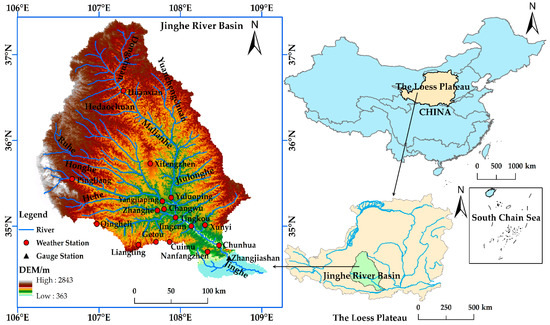
Figure 1.
Geographic location of the JRB and its weather and gauge stations.
The main soil types in the Basin are loessal soil and dark loessal soil, which are thick soil layers (50–80 m), loose in structure, collapse easily, and are eroded [42]. Farm land, forest land, and grassland are three dominant land covers. With the preferential policy of reforestation and revegetation in the late 1990s, the area of cropland in the JRB was gradually reduced and the area of grassland was recovering gradually [43,44].
3. Materials and Methods
3.1. Data Used
The NDVI data for this study, from 1998 to 2018 (1 km spatial resolution), come from the Resources and Environmental Science and Data Center of the Chinese Academy of Sciences (https://www.resdc.cn/ (accessed on 22 November 2022)) [45]. The land use remote sensing data comes from the research results of Yang et al. (https://doi.org/10.5281/zenodo.4417810 (accessed on 22 November 2022)) [46]. The spatial resolution is 30 m. The digital elevation model (DEM) data come from the SRTM (https://earthexplorer.usgs.gov/ (accessed on 22 November 2022)) [47] with a 90 m spatial resolution. The hydrometeorological data, i.e., precipitation, flood runoff, etc., were obtained from the hydrological yearbook and the China Meteorological Data Network (http://data.cma.cn (accessed on 22 November 2022)) [48], which include the measured hydrometeorological data of one controlled hydrological station, and 16 weather stations in the Basin, from 1970 to 2013. The data were used to analyze the changes in the hydrometeorological conditions. The spatial precipitation distribution in the Basin was calculated by inverse distance weighted interpolation (IDW) [49]. The rainstorm and flood data of large, medium, and small typical flood events with good rain–flood relationships were selected for the simulation and statistical analysis.
3.2. Research Content and Technical Route
Based on the long-term NDVI and LUCC time series data, this paper analyzed the time series and spatial distribution change characteristics of the vegetation cover in the JRB. It explored the changing trend of vegetation cover and land use in the Basin, from 1998 to 2018, using the Theil–Sen median trend analysis and Mann–Kendall test (M-K). The time series was separated into the natural and human activity interference periods according to the trend of hydrological and meteorological elements and the inspection and identification characteristics of abrupt change points in the watershed. Finally, a grid-based distributed rainstorm-flood hydrological model simulated and calculated the flooding process in the JRB in different periods. It also studied the flood response characteristics in the Basin under the joint action of long-term climate change and land use/cover change (LUCC). The technological route and research method are shown in Figure 2.
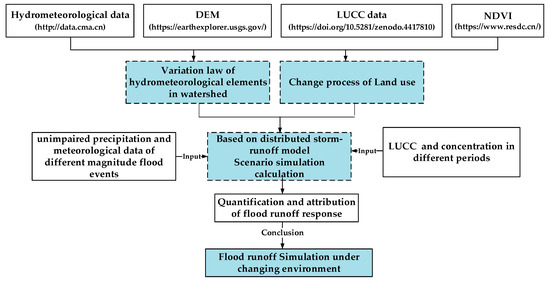
Figure 2.
The technological route and research method employed in the current study.
3.3. Analysis of the Mateo-Hydrological Elements and Underlying Surface Conditions
Combining the Theil–Sen median trend analysis with the M–K test method can allow for judging the long-time series trend of the NDVI [50]. With a strong resistance to data errors, this method does not need time data to obey a specific distribution [51,52].
- (1)
- Theil–Sen median trend analysis with the Mann–Kendall test (M-K)
The Theil–Sen median trend analysis is a non-parametric statistical trend analysis method that can avoid a few outlier influences [53]. For time series , the formula of Sen trend degree β in the Theil–Sen median trend analysis is as follows [54]:
The median is a median function, and when β < 0, it shows a downward trend. When β > 0, it offers an upward trend.
The M–K is a non-parametric statistical test method that can judge the significance of trends [55,56]. This method is widely used to test the trend and mutagenicity of the hydrological series [57]. In this paper, the significance of time series at a 0.05 confidence level is judged by taking the significance level α = 0.05 [58,59].
- (2)
- Cumulative Anomaly Method (CAM)
The CAM can also examine the change points of the hydrological time series [60]. This method is widely used in hydrological research. For the sequence , the cumulative anomaly at time t is expressed as [61]:
where is the value of the hydrological series, m is the time series length, and is the cumulative anomaly at time t. is the mean of the sequence. Drawing curve, the corresponding maximum and the minimum point is the abrupt change point.
3.4. Grid-based Distributed Rainstorm and Flood Model
The modified grid-cell distributed rainfall–runoff (MCDRM) model is a unit distributed rainstorm–runoff model that was developed by the Institute of Disaster Prevention, Kyoto University, Japan, in 2003 [62,63,64]. The Monte Carlo method (MC) was used to obtain the automatic optimization of model parameters in the Basin with the change of underlying surface conditions to reduce the uncertainty of the simulation and calculation of the flooding process [65]. The input data of the model included the topography, hourly precipitation data, land use, etc. The basic principle of the model, considering the human activity interference, is shown in Figure 3.
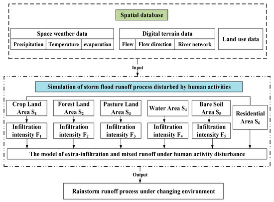
Figure 3.
MCDRM model structure and schematic diagram.
The Basin terrain data of the MCDRM model was represented by the digital elevation model (DEM). Each square grid in the terrain data was a grid cell, and the motion wave equation solved the runoff of the corresponding grid on each grid cell. The model could simulate three lateral flow mechanisms: capillary hole underground flow, non-capillary hole underground flow, and soil surface flow. Darcy’s law was used to simulate the unsaturated seepage in each grid cell. Figure 4 showed the mechanism of the slope runoff generation [66].
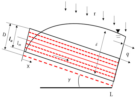
Figure 4.
The diagram of the mechanism of surface–subsurface slope runoff generation.
The average velocity in the direction of the capillary pore gradient was estimated as follows:
where x is the horizontal distance of the grid, m; h is the water head, m; k is unsaturated hydraulic conductivity, m/s. According to the formula of unsaturated hydraulic conductivity [67]: ,i.e., Formula (3) can be rewritten as:
where is the saturated hydraulic conductivity of capillary water, is the saturation, , θ is the water content, is the maximum water content of capillary water, i is the hillside gradient, d is the water level, β is the unsaturated flow constant, is the capillary soil depth, , (D is the soil depth).
When unsaturated , the lateral flow per unit width q of the grid cell:
When saturated, the total flow per unit width q of the grid is calculated from the sum of the capillary flow and gravity flow:
When , to maintain the discharge flux, if the of Formula (5) is equal to that of Formula (6), there are:
When , , is effective porosity, the water flows as surface runoff. Its surface flow average velocity is calculated using the Manning formula:
where n is the Manning roughness coefficient related to the land-use type, and the total flow q is the sum of the surface and groundwater volume:
These three processes can be represented as follows:
The following equation reflects the continuity of the flow of each grid cell:
where T is the time, is the inclination angle, and r is the net rain intensity. The Lax–Wendroff difference scheme solves the 1-D motion wave equation of each node in the grid cell. Figure 5 shows the relationship between the water depth and the unit width discharge (q-d) in each grid [63].
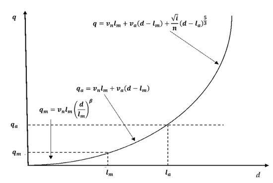
Figure 5.
The relationship between the water depth and the unit width discharge (q-d) in each grid.
3.5. Quantitative Separation of Runoff Response
3.5.1. Unimpaired Precipitation Calculations
The precipitation series with no trend change, compared with the natural period, were obtained by the unimpaired calculation of the flood season precipitation (Pflood season) in the human activity interference period (1979–2013) [68]. In the unimpaired precipitation calculation, first, the linear change ratio of the series was analyzed by the long series annual average data. The linear change ratio was the change quantity of the series. Secondly, the linear change of the series was calculated yearly according to the linear change range of the annual average series. Then, the monthly distribution ratio change was calculated in the natural period. Using the distribution ratio of each month, the distribution and superposition of the annual average change in each month was calculated. Furthermore, the proportion coefficient between the superposition of each month and the actual value was derived. Finally, the scale coefficient of each month in the year was used to scale the actual precipitation amount and precipitation data of the corresponding year and month to obtain the unimpaired Pflood season data.
3.5.2. Quantitative Separation Method of the Hydrological Response
Using the calibrated and validated model, the contribution rate of climate change and human activity interference to the flood change was quantified by inputting the unimpaired precipitation data, the measured precipitation, and the land use data. To clearly describe the separation and quantification process of climate change and human activity interference, the relationship between the variables could be expressed as follows:
where W represents the measured flood volume, W1 represents the flood volume calculated by the measured precipitation and land use data of the corresponding years, W2 represents the flood volume calculated by the unimpaired precipitation and land use data of the corresponding years, W3 represents the flood volume calculated by the unimpaired precipitation and land use data of the natural period, unaffected by climate change and human activity interference, Sseasonal is the high and low change quantity of precipitation, Cclimate is the amount of climate change influence, Hhuman is the amount of human activity interference influence; α is the impact ratio of climate change; β is the influence ratio of human activity interference.
4. Results
4.1. Analysis of the Hydrometeorological Changes
4.1.1. Time Series Variation Characteristics of Precipitation
According to the area average precipitation data for the Basin, from 1970 to 2013, and combining the results of the mutation test by the M–K method and cumulative anomaly method, 1979, 1991, and 1999 were determined as mutation years. The precipitation series in the Basin was divided into natural and human activity interference periods. It was considered that human activity interference in the natural period had relatively little influence on the water cycle and that runoff change was mainly caused by the evolution law of climate change itself. The hydrological process in the human activity interference period was affected by the combined action of climate change and human activity interference. Similarly, the precipitation series in the Basin was divided into natural and anthropogenic periods. Here, the natural period was 1970–1978, while the human activity interference period (I) was 1979–1990, the human activity interference period (II) was 1991–1998, and the human activity interference period (III) was 1999–2013.
4.1.2. Spatial Temporal Variations of Precipitation
The precipitation ratio for the flood season to the annual precipitation in the Basin, from 1970 to 2013, was calculated. From Figure 6, the change in the precipitation proportion for the flood season to the annual precipitation, exhibited stage change characteristics. From 1970 to 1978, the average precipitation growth rate for the flood season to the annual precipitation was 0.1 mm/year. In 1990, the precipitation proportion for the flood season to the annual precipitation decreased by 25.21%, compared to 1979. The proportion of Pflood season to the annual precipitation from 1991 to 1998 and 1999 to 2013, showed an increasing trend. Compared with 1999, the proportion of Pflood season to the annual precipitation in 2013, increased by 29.29%. In 1970–1978, 1979–1990, 1991–1998, and 1999–2013, the average proportion of Pflood season to the annual precipitation was 67.19%, 68.51%, 63.47%, and 68.91%, respectively. Overall, the proportion of Pflood season to the annual precipitation increased, easily leading to rainstorms and flood events.
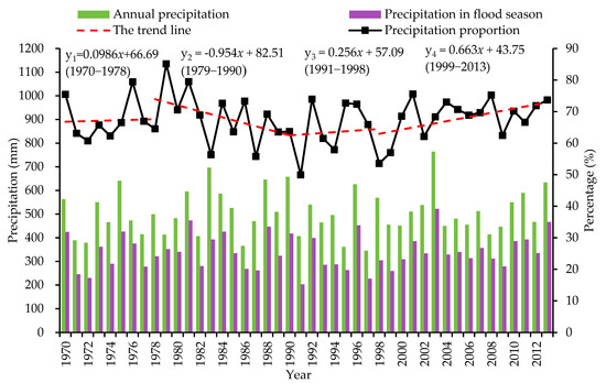
Figure 6.
Trend chart of Pflood season to the annual precipitation in the JRB, from 1970 to 2015; y1: the trend line of the proportion of Pflood season to the annual precipitation in the natural period 1970–1978; y2: the trend line of the proportion of Pflood season to the annual precipitation in the human activity interference period (I) 1979–1990; y3: the trend line of the proportion of Pflood season to the annual precipitation in the human activity interference period (II) 1991–1998; y4: the trend line of the proportion of Pflood season to the annual precipitation in the human activity interference period (III) 1999–2013.
Figure 7 shows the spatial distribution of the precipitation in the Basin. From 1979 to 2013, the Pflood season in the JRB was concentrated in the middle and lower reaches of the Basin, and its spatial distribution was characterized by dynamic stage changes. By comparison, the spatial distribution of Pflood season, in the natural period (1970–1978), was more uniform, and the spatial deviation of precipitation was the historical maximum Cv = 0.11. Compared with the natural period, the spatial precipitation distribution in the human activity interference period is more concentrated, and the spatial deviations of Pflood season in the human activity interference periods (I), (II), and (III) were Cv = 0.09, Cv = 0.04, and Cv = 0.09, respectively. Moreover, the proportion of Pflood season to the annual rainfall in the human activity interference period increased continuously, and precipitation was concentrated within the year. The concentrated spatial distribution of precipitation easily increased the frequency of rainstorms and flood events.
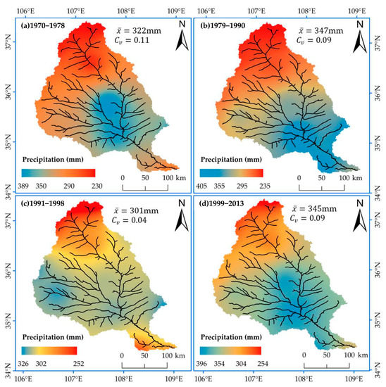
Figure 7.
Spatial distribution map of the precipitation in flood season; (a) natural period 1970–1978; (b) human activity interference period (I) 1979–1990; (c) human activity interference period (II) 1991–1998; (d) human activity interference period (III) 1999–2013.
4.2. Characteristics of the LUCC and NDVI
4.2.1. Analysis Variation of the LUCC
Figure 8 shows LUCC in the human activity interference periods and Figure 9 shows the changes in land types and their area proportions in the study area, from 1985 and 1990–2013. Croplands and pastures predominated the Basin, accounting for 86% of the total basin area. The relationship of the land use types followed the trend: pasture > cropland > forest land > residential area > water area > bare soil. The water and soil conservation and management work in the JRB began in the early 1950s. From 1985 to 2013, the cropland area in the JRB continued to decrease, while the forest land, pastures, and residential areas increased. The environmental improvement effect of reforestation and revegetation in the Basin was pronounced.
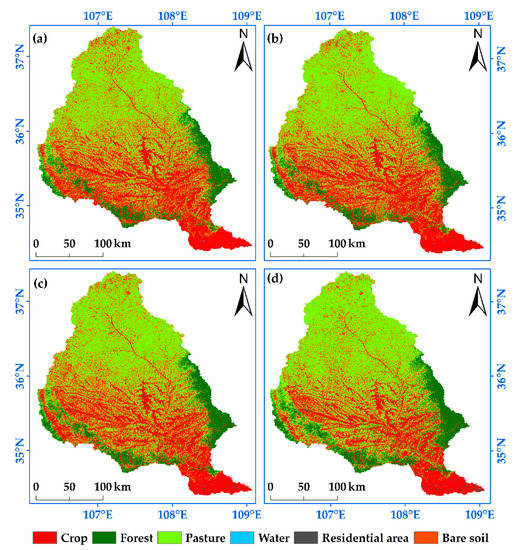
Figure 8.
Land use in the human activity interference periods of the study; (a) land use in 1985; (b) land use in 1991; (c) land use in 1999; (d) land use in 2013.
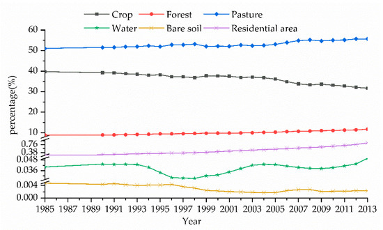
Figure 9.
Change in the proportion of the six land use types, from 1985 to 2013.
Figure 9 and Table 1 illustrate that from 1985 to 2013, the cropland area in the JRB decreased, while forest land, pastures, and residential land increased notably; all changes peaked in 2013. Among them, the forest land area accounted for 12.10% in 2013, 3.24% higher than in 1985; therefore a 36.50% increase. The pasture area accounted for 55.90% in 2013, i.e., 4.84% higher than that in 1985, with rise of 9.42%. The residential land area accounted for 0.92% in 2013, 0.66% higher than in 1985, recording a 259% increase. From 1985 to 2013, the cropland area continued to decrease, accounting for 31.03% in 2013, a decrease of 8.72%, compared with 1985. The proportion of water and the bare land areas barely changed. Based on the time series identification and geographic information systems, the land use transfer matrices of 1985–1991, 1991–1999, and 1999–2013 were made using the land use data of 1985, 1991, 1999, and 2013. Table 2, Table 3 and Table 4 list the results.

Table 1.
Statistics of land use areas in the JRB during 1985–2013.
Table 2.
LUCC transfer matrix of the JRB from 1985 to 1991 (area:km2).
Table 3.
LUCC transfer matrix of the JRB from 1991 to 1999 (area:km2).
Table 4.
LUCC transfer matrix of the JRB from 1999 to 2013 (area:km2).
In 1985 (Table 2), the transferred cropland and pasture areas (1858 and 1717 km2, respectively) were the largest, mainly converted into the forest and residential lands. Compared with 1985, in 1991, all land-use types (except for cropland and bare land) increased in various degrees: pastures increased by 135.1 km2, the forest grew by 18.76 km2, residential land increased by 14.50 km2, water area increased by 1.65 km2, while cropland and bare land decreased by 169.8 km2 and 0.17 km2, respectively.
From Table 3, the cropland area decreased continuously in 1999, and a total of 690 km2 of cropland was transferred out, mainly for residential and forest lands. Furthermore, compared with 1991, the area of forest land, pastures, and residential land in 1999 increased by 364.0, 286.6, and 44.97 km2, respectively, while those of water and bare land decreased by 4.89 and 0.77 km2, respectively.
From 1999 to 2013 (Table 4), the cropland area decreased continuously down to 2679 km2, mainly converted into pastures, forest, and residential lands. By 2013, pastures, forest, and residential lands increased by 1612, 861.5, and 197.7 km2, respectively. Furthermore, the water area increased by 8.65 km2, while the bare land decreased by 0.15 km2.
4.2.2. Analysis Variation of the NDVI
- (1)
- Temporal Variation of the NDVI
The interannual variation of the NDVI value in the JRB, from 1998 to 2018, was counted (Figure 10). The annual average NDVI value in the JRB showed a staged growth trend. The minimum annual average value of the NDVI was 0.449, occurring in 1999. Beginning in 2003, the growth accelerated and peaked at 0.695 in 2018. This continuous increase could be related to reforestation, revegetation, and a series of water conservation measures, since the 1990s.
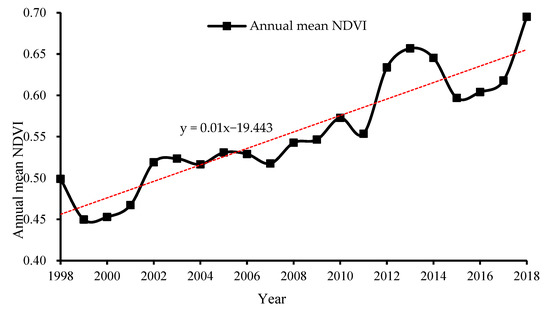
Figure 10.
NDVI changes in the JRB, from 1998 to 2018.
- (2)
- Spatial Variation of the NDVI
Using the NDVI time-series data from 1998 to 2018, the 21-year average NDVI spatial distribution map of the JRB was obtained (Figure 11a). The spatial distribution of the NDVI in the Basin showed that the distribution characteristics were low in the north and high in the south. The area with the highest NDVI (0.75–0.86) accounted for 9.96%, mainly forest land and pastures, as the vegetation thrived. The NDVI value of the Basin ranges from 0.30 to 0.75, accounting for 89.55% of the basin area. The areas with an NDVI value less than 0.30, account for only 0.49%.
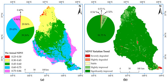
Figure 11.
(a) Spatial distribution of the NDVI mean. (b) Annual mean NDVI variation trend.
According to the actual situation and reference to relevant studies [69], this paper superimposed the results of the Theil–Sen median trend analysis and the M–K test, to obtain the change trend data of the NDVI on a pixel scale. It divided the results into five types (Figure 11b and Table 5). From 1998 to 2018, the improved vegetation coverage area in the JRB was 98.61%, and the degraded area was 1.07%; the improvement effect was remarkable. In the JRB, 91.73% of the Basin significantly improved, while only 1.07% (concentrated in the southern urban areas) was degraded. The continuous and large-scale transformation of the underlying surface conditions of the Basin by human activity interference led to the change in various types of vegetation coverage areas and land use areas. It drove the change in the flooding process and its evolution mechanism.
Table 5.
Trend of the NDVI in the JRB.
4.3. Simulation and the Attribution of Rainstorms and Flood Events under the Changing Environment
4.3.1. Calibration and Verification of the Model Parameters
The distributed storm runoff simulation was constructed by selecting 20 typical rainstorm and flood event data with complete rainfall and flood event data, from 1970 to 2013, in the Basin, among which six flood events were selected from the natural period (1970–1978) and the human activity interference period (I) (1979–1990) to calibrate the model parameters, and five flood events were selected from the human activity interference period (II) (1991–1998) to verify the model. Figure 12 shows the simulation results of four specific flood events. Table 6 lists the model verification results.
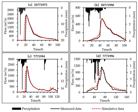
Figure 12.
Diagram of the typical flooding process simulation in the JRB; (a) Date of event onset is 25/7/1975; (b) Date of event onset is 30/7/1990; (c) Date of event onset is 7/7/1994; (d) Date of event onset is 7/7/1996.
Table 6.
Model verification results of the flood simulation of the JRB.
Table 6 shows that the model’s simulation of the peak discharge (Qpeak) and peak time (Tpeak) were relatively accurate. The average relative error of Qpeak of 11 flood events was 0.48%, while the maximum and minimum errors were −1.04% and −0.11%, respectively. The overall simulation results were ideal. The simulation of Tpeak was also accurate, and the simulation error of Tpeak of the flood events was less than 1 h.
Figure 12 depicts that the MCDRM model simulated the sharp and thin flood events (with a steep rise and fall) excellently. Conversely, simulating the multi-peak flood events is poor. Overall, the MCDRM model simulated the flooding process in the JRB. The model was more accurate for short-duration and high intensity precipitation simulations. The poor multi-peak precipitation may be caused by two reasons: (1) the impact of the data processing in the early stage of the model. The model requires that the input precipitation data be generalized into one hour, thus smoothing the flooding process. The study area was consisted mainly of infiltration-excess runoff production. The sudden rise and fall of floods were evident, so the total amount of floods simulated by the model was too large; (2) the uncertainty of model parameters. The model was simple, flexible, and efficient. Although the Monte Carlo module was built to optimize the parameters, and the simulation principle of giving priority to the Tpeak and Qpeak accuracy was set simultaneously, the change interval of the parameters was still uncertain.
4.3.2. Quantifying the Impact of Climate Change and LUCC on Floods
Using the calibrated and validated model, the contribution rate of LUCC and climate change to flood change was quantitatively calculated by inputting the unimpaired precipitation data, the measured precipitation and the land use data in the natural period. For the convenience of expression, Q represents the measured Qpeak, Q1 represents the Qpeak calculated by the measured precipitation and land use data, Q2 represents the Qpeak calculated by the unimpaired precipitation and land use data of the corresponding years, and Q3 represents the Qpeak calculated by the unimpaired precipitation and land use data of the natural period. W represents the measured flood volume, W1 represents the flood volume calculated by the measured precipitation and land use data, and W2 represents the flood volume calculated by the unimpaired precipitation and land use data of the corresponding years. In contrast, W3 represents the flood volume calculated by the unimpaired precipitation and land use data of the natural period. According to the K-means clustering method, and referring to the actual situation of the Basin, the flood magnitude was divided into three levels: large flood, medium flood, and small flood. Among them, a small, medium, and the large flood has a Qpeak of <1200, 1200–2300, and >2300 m3/s, respectively. The simulation results of the rainstorms and floods under various underlying surface and meteorological conditions are provided in Table 7. Figure 13 shows the simulation result of the flooding process in the Basin under the changing environment.
Table 7.
Simulation of the JRB under the changing environment.
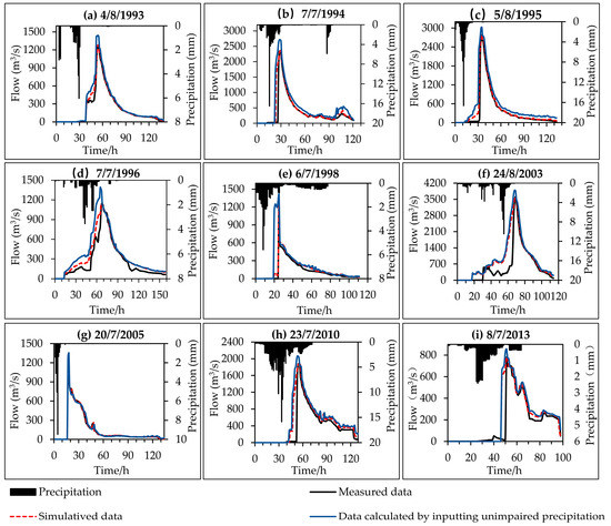
Figure 13.
Simulation diagram of the flooding process in the Basin under the changing environment; (a) Date of event onset is 4/8/1993; (b) Date of event onset is 7/7/1994; (c) Date of event onset is 5/8/1995; (d) Date of event onset is 7/7/1996; (e) Date of event onset is 6/7/1998; (f) Date of event onset is 24/8/2003; (g) Date of event onset is 20/7/2005; (h) Date of event onset is 23/7/2010; (i) Date of event onset is 8/7/2013.
As illustrated in Table 7, the simulated Qpeak and flood volume in the period unaffected by LUCC and climate change were larger than the measured data. Furthermore, LUCC and climate change had a pronounced peak clipping effect on the flooding process, among which the Qpeak change ratio was between 8% and 22%. Specifically, the Qpeak change ratio of 21.8% in 7/7/1996 was the largest. Because the precipitation in the JRB is primarily a short-duration rainstorm, and the flood pattern is mostly very thin, the flood pattern does not change significantly before and after the change in precipitation and land use. Furthermore, the attenuation of the flood volume was mainly affected by the Qpeak attenuation. The change ratio of the flood volume range was 5–67%, and the change ratio of the flood volume in 19950805 floods (66.45%) was the largest.
Table 8 lists the quantitative results of the flood response to climate change and LUCC in the JRB. The results showed that climate change contributed >60% to floods in different flood magnitudes due to climate change and LUCC. The average contribution of climate change to small, medium, and large floods was 66.29%, 81.58%, and 70.12%, respectively. The average contribution rate of LUCC to small, medium, and large floods was 33.71%, 18.41%, and 29.88%, which indicated that the impact of LUCC on the flood was inversely proportional to the flood magnitude. With the increase in rainstorm intensity, the impact of LUCC on the flooding process gradually decreased. For large and medium-sized floods, the rainstorm intensity had a more significant effect.
Table 8.
Quantitative calculation of the influence of climate change and LUCC on floods in the JRB.
5. Discussion
- (1)
- By analyzing the spatial temporal changes of the hydrometeorological elements, the normalized difference vegetation index and land use/cover change data, the hydrological sequence was split into natural and human activity interference periods. From 1979 to 2013, the Pflood season in the JRB was concentrated in the middle and lower reaches of the Basin, and its spatial distribution showed periodic dynamic changes. Compared with the natural period, the proportion of Pflood season to the annual precipitation in the human activity interference period increased consistently;
- (2)
- Normalized difference vegetation index (NDVI) showed an upward trend at a rate of 0.01 a−1 during 1998 and 2018. The spatial distribution of the NDVI was heterogeneous in the study area. Combined with the historical land-use situation in the study area, the cropland area in the JRB continued to decrease, while the forest land, pastures, and residential areas increased. In the 1950s, the water and soil conservation and management work began in the Basin. The environmental improvement effect of reforestation and revegetation was noticeable. Since, 91.73% of the JRB area has improved the vegetation coverage, while only 1.07% of the area has degraded, especially in the southern urban areas of the Basin. The continuous large-scale transformation of the underlying surface conditions of the Basin has led to the various types of land use and vegetation coverage areas. It drove the change in the flooding process and its evolution mechanism;
- (3)
- The joint impact of LUCC and climate change has significantly lowered the Qpeak and flood volume in the JRB, from 1999 to 2013. Affected by climate change, the precipitation proportion during the flood season to the annual precipitation in other periods increased steadily, readily causing an increase in the frequency of rainstorms and flood events. However, due to the enhancement of flood regulation and storage caused by the transformation of the underlying surface conditions by human activity interference, the Qpeak and the flood volume are still decreasing in the current situation;
- (4)
- The distributed storm flood model (MCDRM) revealed that the contribution rate of climate change to the flood volume reduction of different magnitude flood events followed the trend: medium flood > large flood > small flood. The shift in the runoff process of the medium and large floods was mainly driven by climate change, while anthropogenic and climate change impacts on the change of small floods were identical. Since 1994, the influence of climate change on the flood runoff change gradually weakened, while the effect of LUCC on the flood runoff change increased obviously.
6. Conclusions
In this study, the distributed hydrological model excellently simulated the flood Qpeak and peak occurrence times, showing meager errors. In constructing the MCDRM model, the distribution of the hydrological and meteorological observation stations, LUCCs were fully considered to reduce the uncertainty caused by the data input. Meanwhile, we also optimized the model algorithm to reduce the model simulation’s uncertainty. However, geological hazards within the Basin and internal water migration were not considered, such as the impact of landslides, irrigation pumping, and wastewater discharge on the local hydrological cycle, which bring uncertainty to the simulation results of the model.
With the increase of human activities in the Loess Plateau region, the evolution mechanism of the flood process will become more complicated and the uncertainty of flood simulations will increase. Therefore, it is necessary to study the runoff evolution mechanism affected by typical human activities, and optimize the structure of the model accordingly, to improve the simulation accuracy of the model in the follow-up research.
Author Contributions
All authors contributed to the work. J.L. conceived and designed the study, S.Y. and K.W. performed the computations and data analysis; Y.S. provided the data; P.L. and X.M. proofread and edited the manuscript. All authors have read and agreed to the published version of the manuscript.
Funding
This research was funded by the Shaanxi Postdoctoral Science Foundation 2018 (2018BSHEDZZ21), the National Natural Foundation of China (51679185), the General Financial Grant from the China Postdoctoral Science Foundation (2017M623088), and the Yinshanbeilu Grassland Eco-hydrology National Observation and Research Station, China Institute of Water Resources and Hydropower Research, Beijing 100038, China (YSS2022004). The APC was funded by the Fundamental Research Funds for the Central Universities, CHD (300102292903).
Data Availability Statement
Data used in this study are duly available from the first author on reasonable request.
Acknowledgments
The authors would like to thank the editors and the reviewers for their crucial comments and suggestions, which improved the quality of this paper.
Conflicts of Interest
The authors declare no conflict of interest.
References
- Huntington, T.G. Evidence for intensification of the global water cycle: Review and synthesis. J. Hydrol. 2006, 319, 83–95. [Google Scholar] [CrossRef]
- Hegerl, G.C.; Black, E.; Allan, R.P.; Ingram, W.J.; Polson, D.; Trenberth, K.E.; Chadwick, R.S.; Arkin, P.A.; Sarojini, B.B.; Becker, A.; et al. Challenges in Quantifying Changes in the Global Water Cycle. Bull. Amer. Meteorol. Soc. 2015, 96, 1097–1115. [Google Scholar] [CrossRef]
- Sun, P.; Wen, Q.Z.; Zhang, Q.; Singh, V.P.; Sun, Y.Y.; Li, J.F. Nonstationarity-based evaluation of flood frequency and flood risk in the Huai River basin, China. J. Hydrol. 2018, 567, 393–404. [Google Scholar] [CrossRef]
- Lyu, J.; Mo, S.; Luo, P.; Zhou, M.; Shen, B.; Nover, D. A quantitative assessment of hydrological responses to climate change and human activities at spatiotemporal within a typical catchment on the Loess Plateau, China. Quat. Int. 2019, 527, 1–11. [Google Scholar] [CrossRef]
- Desta, H.; Lemma, B.; Gebremariam, E. Identifying sustainability challenges on land and water uses: The case of Lake Ziway watershed, Ethiopia. Appl. Geogr. 2017, 88, 130–143. [Google Scholar] [CrossRef]
- Zhang, M.; Wei, X. The effects of cumulative forest disturbance on streamflow in a large watershed in the central interior of British Columbia, Canada. Hydrol. Earth Syst. Sci. 2012, 16, 2021–2034. [Google Scholar] [CrossRef]
- Sujing, C.; Lijuan, L.; Jiuyi, L.; Jiaxu, L. Impacts of Climate Change and Human Activities on Water Suitability in the Upper and Middle Reaches of the Taoer River Area. J. Resour. Ecol. 2016, 7, 378–385. [Google Scholar] [CrossRef]
- Zou, Y.; Sun, P.; Ma, Z.; Lv, Y.; Zhang, Q. Snow Cover in the Three Stable Snow Cover Areas of China and Spatio-Temporal Patterns of the Future. Remote Sens. 2022, 14, 3098. [Google Scholar] [CrossRef]
- Vanwalleghem, T.; Gomez, J.A.; Infante Amate, J.; Gonzalez de Molina, M.; Vanderlinden, K.; Guzman, G.; Laguna, A.; Giraldez, J.V. Impact of historical land use and soil management change on soil erosion and agricultural sustainability during the Anthropocene. Anthropocene 2017, 17, 13–29. [Google Scholar] [CrossRef]
- Cui, Q.-Y.; Gaillard, M.-J.; Lemdahl, G.; Stenberg, L.; Sugita, S.; Zernova, G. Historical land-use and landscape change in southern Sweden and implications for present and future biodiversity. Ecol. Evol. 2014, 4, 3555–3570. [Google Scholar] [CrossRef]
- Jaiswal, M.K.; Amin, N. Impact of land-use land cover dynamics on runoff in Panchnoi River basin, North East India. Geoscape 2021, 15, 19–29. [Google Scholar] [CrossRef]
- Dwarakish, G.S.; Ganasri, B.P. Impact of land use change on hydrological systems: A review of current modeling approaches. Cogent Geosci. 2015, 1, 1115618–1115691. [Google Scholar] [CrossRef]
- Li, P.; Li, H.; Yang, G.; Zhang, Q.; Diao, Y. Assessing the Hydrologic Impacts of Land Use Change in the Taihu Lake Basin of China from 1985 to 2010. Water 2018, 10, 1512. [Google Scholar] [CrossRef]
- Wang, S.; Luo, P.; Xu, C.; Zhu, W.; Cao, Z.; Ly, S. Reconstruction of Historical Land Use and Urban Flood Simulation in Xi’an, Shannxi, China. Remote Sens. 2022, 14, 6067. [Google Scholar] [CrossRef]
- Wang, G.Q.; Zhang, J.Y.; Xuan, Y.Q.; Liu, J.F.; Jin, J.L.; Bao, Z.X.; He, R.M.; Liu, C.S.; Liu, Y.L.; Yan, X.L. Simulating the Impact of Climate Change on Runoff in a Typical River Catchment of the Loess Plateau, China. J. Hydrometeorol. 2013, 14, 1553–1561. [Google Scholar] [CrossRef]
- Bojie, F.; Shuai, W.; Yu, L.; Jianbo, L.; Wei, L.; Chiyuan, M. Hydrogeomorphic Ecosystem Responses to Natural and Anthropogenic Changes in the Loess Plateau of China. Annu. Rev. Earth Planet. Sci. 2017, 45, 223–243. [Google Scholar] [CrossRef]
- Shi, H.; Shao, M. Soil and water loss from the Loess Plateau in China. J. Arid. Environ. 2000, 45, 9–20. [Google Scholar] [CrossRef]
- Liu, Z.P.; Wang, Y.Q.; Shao, M.G.; Jia, X.X.; Li, X.L. Spatiotemporal analysis of multiscalar drought characteristics across the Loess Plateau of China. J. Hydrol. 2016, 534, 281–299. [Google Scholar] [CrossRef]
- Wang, G.; Zhang, J.; Yang, Q. Attribution of Runoff Change for the Xinshui River Catchment on the Loess Plateau of China in a Changing Environment. Water 2016, 8, 267. [Google Scholar] [CrossRef]
- Wang, S.T.; Cao, Z.; Luo, P.P.; Zhu, W. Spatiotemporal Variations and Climatological Trends in Precipitation Indices in Shaanxi Province, China. Atmosphere 2022, 13, 744. [Google Scholar] [CrossRef]
- Zhang, L.; Nan, Z.; Xu, Y.; Li, S. Hydrological Impacts of Land Use Change and Climate Variability in the Headwater Region of the Heihe River Basin, Northwest China. PLoS ONE 2016, 11, e0158394. [Google Scholar] [CrossRef] [PubMed]
- Yang, Y.; Zhu, Y.; Shao, S. Review on ecohydrological processes in Loess Plateau. Acta Ecol. Sin. 2018, 38, 4052–4063. [Google Scholar] [CrossRef]
- Li, Q.; Sun, Y.; Yuan, W.; Lyu, S.; Wan, F. Streamflow responses to climate change and LUCC in a semi-arid watershed of Chinese Loess Plateau. J. Arid. Land 2017, 9, 609–621. [Google Scholar] [CrossRef]
- Taffi, M. Effects of climate change and human activities on runoff in the Beichuan River Basin in the northeastern Tibetan Plateau, China (vol 176, pg 81, 2019). Catena 2019, 177, 286. [Google Scholar] [CrossRef]
- Sun, P.; Zhang, Q.; Gu, X.H.; Shi, P.J.; Singh, V.; Song, C.Q.; Zhang, X.Y. Nonstationarities and At-site Probabilistic Forecasts of Seasonal Precipitation in the East River Basin, China. Int. J. Disaster Risk Sci. 2018, 9, 100–115. [Google Scholar] [CrossRef]
- Ashofteh, P.S.; Bozorg-Haddad, O.; Loaiciga, H.A.; Marino, M.A. Evaluation of the Impacts of Climate Variability and Human Activity on Streamflow at the Basin Scale. J. Irrig. Drain. Eng. 2016, 142, 04016028. [Google Scholar] [CrossRef]
- Luo, P.; Zheng, Y.; Wang, Y.; Zhang, S.; Yu, W.; Zhu, X.; Huo, A.; Wang, Z.; He, B.; Nover, D. Comparative Assessment of Sponge City Constructing in Public Awareness, Xi’an, China. Sustainability 2022, 14, 11653. [Google Scholar] [CrossRef]
- Luo, P.; Luo, M.; Li, F.; Qi, X.; Huo, A.; Wang, Z.; He, B.; Takara, K.; Nover, D.; Wang, Y. Urban flood numerical simulation: Research, methods and future perspectives. Environ. Model. Softw. 2022, 156, 105478. [Google Scholar] [CrossRef]
- Zhu, W.; Zha, X.B.; Luo, P.P.; Wang, S.T.; Cao, Z.; Lyu, J.Q.; Zhou, M.M.; He, B.; Nover, D. A quantitative analysis of research trends in flood hazard assessment. Stoch. Environ. Res. Risk Assess. 2023, 37, 413–428. [Google Scholar] [CrossRef]
- Zhu, Y.; Luo, P.; Zhang, S.; Sun, B. Spatiotemporal Analysis of Hydrological Variations and Their Impacts on Vegetation in Semiarid Areas from Multiple Satellite Data. Remote Sens. 2020, 12, 4177. [Google Scholar] [CrossRef]
- Wang, G.; Xia, J.; Chen, J. Quantification of effects of climate variations and human activities on runoff by a monthly water balance model: A case study of the Chaobai River basin in northern China. Water Resour. Res. 2009, 45, W00A11. [Google Scholar] [CrossRef]
- Hu, C.; Zhang, L.; Wu, Q.; Soomro, S.-E.-H.; Jian, S. Response of LUCC on Runoff Generation Process in Middle Yellow River Basin: The Gushanchuan Basin. Water 2020, 12, 1237. [Google Scholar] [CrossRef]
- Guo, P.; Lyu, J.; Yuan, W.; Zhou, X.; Mo, S.; Mu, D.; Luo, P. Detecting the Quantitative Hydrological Response to Changes in Climate and Human Activities at Temporal and Spatial Scales in a Typical Gully Region of the Loess Plateau, China. Water 2022, 14, 257. [Google Scholar] [CrossRef]
- Guo, J.; Zhang, Z.; Wang, S.; Strauss, P.; Yao, A. Appling SWAT model to explore the impact of changes in land use and climate on the streamflow in a Watershed of Northern China. Acta Ecol. Sin. 2014, 34, 1559–1567. [Google Scholar] [CrossRef]
- Wu, J.; Miao, C.; Wang, Y.; Duan, Q.; Zhang, X. Contribution analysis of the long-term changes in seasonal runoff on the Loess Plateau, China, using eight Budyko-based methods. J. Hydrol. 2016, 545, 263–275. [Google Scholar] [CrossRef]
- Chen, H.; Fleskens, L.; Baartman, J.; Wang, F.; Moolenaar, S.; Ritsema, C. Impacts of land use change and climatic effects on streamflow in the Chinese Loess Plateau: A meta-analysis. Sci. Total Environ. 2020, 703, 15. [Google Scholar] [CrossRef] [PubMed]
- Zhang, J.L.; Shang, Y.Z.; Liu, J.Y.; Fu, J.; Wei, S.T.; Tong, L. Causes of Variations in Sediment Yield in the Jinghe River Basin, China. Sci. Rep. 2020, 10, 18. [Google Scholar] [CrossRef]
- Xu, B.; Pan, J. Simulation and measurement of soil conservation service flow in the Loess Plateau: A case study for the Jinghe River Basin, Northwestern China. Ecol. Indic. 2022, 141, 109072. [Google Scholar] [CrossRef]
- Zheng, T.; Zhou, Z.X.; Zou, Y.F.; Pulatov, B.; Biswas, A. Analysis of Spatial and Temporal Characteristics and Spatial Flow Process of Soil Conservation Service in Jinghe Basin of China. Sustainability 2021, 13, 1794. [Google Scholar] [CrossRef]
- Zhao, L.; Lu, A.F.; Wu, J.J.; Hayes, M.; Tang, Z.H.; He, B. The Impact of Meteorological Drought on Streamflow in the Jinghe River basin of China. In Proceedings of the 13th International Conference on Environmental Science and Technology (CEST), Athens, Greece, 5–7 September 2013. [Google Scholar]
- Zha, X.; Huang, C.; Pang, J.; Li, Y. Sedimentary and hydrological studies of the Holocene palaeofloods in the middle reaches of the Jinghe River. J. Geogr. Sci. 2012, 22, 470–478. [Google Scholar] [CrossRef]
- Peng, H.; Jia, Y.; Niu, C.; Gong, J.; Hao, C.; Gou, S. Eco-hydrological simulation of soil and water conservation in the Jinghe River Basin in the Loess Plateau, China. J. Hydro Environ. Res. 2015, 9, 452–464. [Google Scholar] [CrossRef]
- Ran, D.C.; Shen, Z.Z.; Zeng, M.L. The analysis of relationships between rainfall and warp dam block sediment in Jinghe watershed. In Proceedings of the 1st International Conference on Energy and Environmental Protection (ICEEP 2012), Hohhot, China, 23–24 June 2012; pp. 4653–4660. [Google Scholar]
- Jing, C.; Jianguo, S.; Tao, L. Runoff Simulation in Jinghe River Basin Based on the SWAT Model. In Proceedings of the 2012 International Symposium on Geomatics for Integrated Water Resource Management, Lanzhou, China, 19–21 October 2012; pp. 1–3. [Google Scholar]
- Spatial Distribution Data Set of Annual Vegetation Index (NDVI) in China Data Registration and Publishing System of Data Center of Resources and Environment Science. Available online: https://www.resdc.cn/ (accessed on 22 November 2022).
- Yang, J.; Huang, X. The 30 m annual land cover dataset and its dynamics in China from 1990 to 2019. Earth Syst. Sci. Data 2021, 13, 3907–3925. [Google Scholar] [CrossRef]
- Nima, N. STRM3 DEM. Available online: https://earthexplorer.usgs.gov/ (accessed on 22 November 2022).
- Center, C.M.D.S.C.N.M.I. Hourly Data from Surface Meteorological Stations in China. Available online: http://data.cma.cn/ (accessed on 21 November 2022).
- Bartier, P.M.; Keller, C.P. Multivariate interpolation to incorporate thematic surface data using inverse distance weighting (IDW). Comput. Geosci. 1996, 22, 795–799. [Google Scholar] [CrossRef]
- Bo-feng, C.A.I.; Rong, Y.U. Advance and evaluation in the long time series vegetation trends research based on Remote Sens. J. Remote Sens. 2009, 13, 1170–1186. [Google Scholar] [CrossRef]
- Lunetta, R.S.; Knight, J.F.; Ediriwickrema, J.; Lyon, J.G.; Worthy, L.D. Land-cover change detection using multi-temporal Modis Ndvi data. Remote Sens. Environ. 2006, 105, 142–154. [Google Scholar] [CrossRef]
- Milich, L.; Weiss, E. GAC NDVI interannual coefficient of variation (CoV) images: Ground truth sampling of the Sahel along north-south transects. Int. J. Remote Sens. 2000, 21, 235–260. [Google Scholar] [CrossRef]
- Tucker, C.J.; Newcomb, W.W.; Los, S.O.; Prince, S.D. Mean and inter-year variation of growing-season normalized difference vegetation index for the Sahel 1981–1989. Int. J. Remote Sens. 1991, 12, 1133–1135. [Google Scholar] [CrossRef]
- da Silva, R.M.; Santos, C.A.G.; Moreira, M.; Corte-Real, J.; Silva, V.C.L.; Medeiros, I.C. Rainfall and river flow trends using Mann-Kendall and Sen’s slope estimator statistical tests in the Cobres River basin. Nat. Hazards 2015, 77, 1205–1221. [Google Scholar] [CrossRef]
- Chebana, F.; Ouarda, T.B.M.J.; Thuy Chinh, D. Testing for multivariate trends in hydrologic frequency analysis. J. Hydrol. 2013, 486, 519–530. [Google Scholar] [CrossRef]
- Tosic, I. Spatial and temporal variability of winter and summer precipitation over Serbia and Montenegro. Theor. Appl. Climatol. 2004, 77, 47–56. [Google Scholar] [CrossRef]
- Zhang, D.; Liu, X.M.; Liu, C.M.; Bai, P. Responses of runoff to climatic variation and human activities in the Fenhe River, China. Stoch. Environ. Res. Risk Assess. 2013, 27, 1293–1301. [Google Scholar] [CrossRef]
- Bao, Z.X.; Zhang, J.Y.; Wang, G.Q.; Fu, G.B.; He, R.M.; Yan, X.L.; Jin, J.L.; Liu, Y.L.; Zhang, A.J. Attribution for decreasing streamflow of the Haihe River basin, northern China: Climate variability or human activities? J. Hydrol. 2012, 460, 117–129. [Google Scholar] [CrossRef]
- Liu, X.M.; Liu, C.M.; Luo, Y.Z.; Zhang, M.H.; Xia, J. Dramatic decrease in streamflow from the headwater source in the central route of China’s water diversion project: Climatic variation or human influence? J. Geophys. Res.-Atmos. 2012, 117, 10. [Google Scholar] [CrossRef]
- Ran, L.; Wang, S.; Fan, X. Channel change at Toudaoguai Station and its responses to the operation of upstream reservoirs in the upper Yellow River. J. Geogr. Sci. 2010, 20, 231–247. [Google Scholar] [CrossRef]
- Zhao, L.; Tang, P.; Huang, S.; Zhang, W. Analysis on the Variation Characteristics of Temperature in Wengyuan from 1961 to 2018. Meteorol. Environ. Res. 2022, 13, 25–27+36. [Google Scholar] [CrossRef]
- Kim, S.; Tachikawa, Y.; Sayama, T.; Takara, K. Ensemble flood forecasting with stochastic radar image extrapolation and a distributed hydrologic model. Hydrol. Process. 2009, 23, 597–611. [Google Scholar] [CrossRef]
- Kojima, T.; Takara, K. A grid-cell based distributed flood runoff model and its performance. Weather. Radar Inf. Distrib. Hydrol. Model. 2003, 2003, 234–240. [Google Scholar]
- Sayama, T.; McDonnell, J.J. A new time-space accounting scheme to predict stream water residence time and hydrograph source components at the watershed scale. Water Resour. Res. 2009, 45, W07401. [Google Scholar] [CrossRef]
- Sayama, T.; Takara, K.; Tachikawa, Y. Reliability Evaluation of Rainfall-Sedi Ment-Runoff Models; IAHS Publications: Wallingford, UK, 2003; Volume 279, pp. 131–141. [Google Scholar]
- Sayama, T.; Tachikawa, Y.; Takara, K. Spatial lumping of a distributed rainfall-sediment-runoff model and its effective lumping scale. Hydrol. Process. 2012, 26, 855–871. [Google Scholar] [CrossRef]
- Gardner, W.R. Dynamic Aspects of Soil-Water Availability to Plants. Annu. Rev. Plant Physiol. 1965, 16, 323–342. [Google Scholar] [CrossRef]
- Jiang, S.; Ren, L.; Yong, B.; Fu, C.; Yang, X. Analyzing the effects of climate variability and human activities on runoff from the Laohahe basin in northern China. Hydrol. Res. 2012, 43, 3–13. [Google Scholar] [CrossRef]
- Lihua, Y.; Weiguo, J.; Wenming, S.; Yinghui, L.; Wenjie, W.; Liangliang, T.; Hua, Z.; Xiaofu, L. The spatio-temporal variations of vegetation cover in the Yellow River Basin from 2000 to 2010. Acta Ecol. Sin. 2013, 33, 7798–7806. [Google Scholar] [CrossRef]
Disclaimer/Publisher’s Note: The statements, opinions and data contained in all publications are solely those of the individual author(s) and contributor(s) and not of MDPI and/or the editor(s). MDPI and/or the editor(s) disclaim responsibility for any injury to people or property resulting from any ideas, methods, instructions or products referred to in the content. |
© 2023 by the authors. Licensee MDPI, Basel, Switzerland. This article is an open access article distributed under the terms and conditions of the Creative Commons Attribution (CC BY) license (https://creativecommons.org/licenses/by/4.0/).