Analyzing the Ionospheric Irregularities Caused by the September 2017 Geomagnetic Storm Using Ground-Based GNSS, Swarm, and FORMOSAT-3/COSMIC Data near the Equatorial Ionization Anomaly in East Africa

Abstract

Geomagnetic storms are one of the leading causes of ionospheric irregularities, depending on their intensity. The 6–10 September 2017 geomagnetic storm, the most severe geomagnetic event of the year, resulted from an X9 solar flare and a subsequent coronal mass ejection (CME), with the first sudden storm commencements (SSC) occurring at 23:43 UT on day 06, coinciding with a Sym-H value of approximately 50 nT, triggered by a sudden increase in the solar wind. The interplanetary magnetic field (IMF) and disturbance storm time (Dst) increased when the first SSC occurred at 23:43 UT on 6 September. The second SSC occurred with a more vigorous intensity at 23:00 UT on 7 September, with the Kp index reaching 8 and the auroral electrojet (AE) 2500 nT. In this study, we investigated this phenomenon using data from Swarm, FORMOSAT-3/COSMIC, and ground-based GNSS networks in East Africa to measure ionospheric irregularities near the equatorial ionization anomaly (EIA). In this procedure, the total electron content (TEC), amplitude scintillation (S4), and rate of TEC Index (ROTI) were implemented to recognize ionospheric irregularities appearing during the geomagnetic storm. In addition, the Langmuir plasma probes of the Swarm satellites were employed to identify the rate of electron density index (RODI). The results obtained from the different techniques indicate the effects of geomagnetic storms in terms of increased ionospheric irregularities indicated by geophysical ionospheric parameters. This study demonstrates the potential of using space-based measurements to detect the effects of a geomagnetic storm on ionospheric irregularities for regions where ground-based ionospheric observations are rarely available, such as above the oceans.

1. Introduction

Geomagnetic perturbations, which reach their peak during geomagnetic storms, have a profound impact on the ionosphere, causing irregular and severe variations in its structure. These disturbances represent a significant phenomenon influencing the ionosphere and are triggered by the collision of intense solar winds with the interplanetary magnetic field within Earth’s magnetosphere [1]. The structure of the ionosphere undergoes disturbances due to dynamic and electrodynamic processes occurring at different phases of geomagnetic storms. The effects manifest in two distinct phases, the first of which generates an electric field in the ionosphere known as a prompt penetration electric field (PPEF) [2]. A PPEF induces an electric shear flow that rapidly expands from high-latitude to medium and low-latitude regions. In low-latitude regions, the impact of this electric field is temporally dependent, with the PPEF exhibiting an eastward trend during the day and westward after 9 P.M. local time. Following sunset, the post-sunset effects of a PPEF in EIA regions accelerate the ionospheric layers vertically, affecting the height of the F layer [3]. During geomagnetic storms, a PPEF serves as the primary source of large-scale perturbations in the evening. Consequently, the electron density gradient in the lower layers of the ionosphere increases, leading to the growth of ionospheric plasma bubbles. This expansion is a result of the unstable Rayleigh–Taylor process, generating ionospheric perturbations. The upward movement of ionospheric plasma bubbles occurs at the $\overline{\mathrm{E}}\times \overline{\mathrm{B}}$ drift velocity, driven by their polarization electric field, where $\overline{\mathrm{E}}$ and $\overline{\mathrm{B}}$ represent the electric and magnetic fields, respectively [4].

While geomagnetic storms are commonly associated with heightened ionospheric perturbations, they can also exert inhibitory effects on the generation of equatorial plasma bubbles (EPBs) under specific conditions. The increased ionospheric disturbance dynamics, particularly those attributed to a PPEF, can influence the vertical motion of the ionospheric layers, contributing to EPB formation [4]. However, in instances where geomagnetic storms suppress the ionospheric instabilities responsible for EPB generation, inhibitory effects may prevail. Factors such as intensified electric fields or altered dynamo processes during specific storm phases can act as inhibitory mechanisms, impacting the growth and development of EPBs [1,4]. Understanding the intricate interactions between geomagnetic storms and EPB generation requires a nuanced consideration of various physical processes in the ionosphere, with the delicate interplay contingent on specific conditions, including the strength, duration, and temporal evolution of geomagnetic perturbations [4].

Known as the recovery phase, the third phase of geomagnetic storms can influence the ionospheric structure over varying durations, ranging from a few hours for short-term irregularities to several days for long-term irregularities. These perturbations arise from the ionospheric disturbance dynamo [5,6]. After the main phase of a geomagnetic storm, high-energy particles in the ionosphere move from high latitudes to medium and low latitudes, following a disturbance dynamo electric field (DDEF) that expands in equatorial regions [7]. This electric field can behave differently depending on the time of day, moving west during the day and east at night, in an inverse manner to a PPEF [8]. As a consequence of the DDEF behavior during the day in the EIA regions, the F layer height and the rate of occurrence of ionospheric plasma bubbles decrease. However, this electric field changes its behavior during the night, when it increases the ionosphere movement rate, causing ionospheric perturbations [9].

Ionospheric perturbations are caused by a combination of factors that can be analyzed through electron density observations, the rate of change of the electron density, and ionospheric scintillation parameters [10]. The patterns of electron density perturbations and ionospheric irregularities depend on how the PPEF and the DDEF react during the two geomagnetic storm phases [11]. Geomagnetic storms can strengthen the recombination process, weaken the ionization process in the ionosphere, and start the ionospheric plasma depletion.

Two distinct mechanisms contribute to the generation of negative ionosphere storms during geomagnetic disturbances. The first mechanism involves a chemical factor, wherein a reduction of the oxygen (O) to nitrogen (N₂) density ratio (O/N₂) occurs due to upwelling induced by heightened Joule heating in the polar region. The subsequent depletion of O/N₂ is then propelled equatorward by an intensified equatorward wind, leading to a consequential reduction in the electron density [12]. The second mechanism entails the poleward transport of plasma along magnetic field lines, facilitating the movement of ionospheric constituents from higher to lower altitudes [13]. This poleward wind-induced transport mechanism operates independently but concurrently with the chemical factor, contributing to the overall manifestation of negative ionosphere storms during geomagnetic perturbations. This dual-pronged approach, elucidated by Cai et al. [12] and Liu et al. [13], underscores the complexity of the processes involved in the genesis of negative ionosphere storms. The chemical alteration of O/N₂ ratios and the orchestrated movement of plasma along magnetic field lines collectively contribute to the observed disturbances in the ionospheric environment during geomagnetic storms. This nuanced understanding advances our comprehension of the multifaceted dynamics underlying ionospheric variations in response to solar–terrestrial interactions.

The behavior of a geomagnetic storm can increase the electron density (N_e), total electron content (TEC), and ionospheric irregularities, such as ionospheric scintillations that will cause disturbances in the radio signals passing through this medium [14]. The depleted plasma, in combination with the dense plasma in the ionosphere, creates a strong gradient in the ionospheric structure, thereby causing ionospheric irregularities such as ionospheric scintillations near equatorial latitudes [15,16]. The ionospheric scintillation of plasma perturbations can lead to disturbances in amplitude and phase signals that can cause a loss of GNSS lock and produce global navigation satellite system (GNSS) positioning errors in low latitudes, which is more likely to occur after sunset [17]. Ionospheric irregularities produce disturbances related to the local time, season, solar activity, and geomagnetic activity; hence, ionospheric perturbations change such indices as Dst, AE, and d(Dst)/dt (the rate of Dst variation). These parameters can be employed to determine the effects of geomagnetic perturbations [18].

Ground-based GNSS observations show variations in ionospheric parameters on the GNSS signal path. It is also essential to employ observations of the upper ionosphere because thermal plasma emission along the magnetic field can play a crucial role in electron density variations in the upper ionosphere [19]. Nearly two-thirds of TEC observations and their perturbations occur within the F2 layer at the top of the ionosphere, which can be used during ionospheric perturbations such as geomagnetic storms [20]. Several low earth orbit (LEO) satellites, such as the Swarm mission and FORMOSAT-3/COSMIC (F3/C) satellites, have been launched in recent years to detect ionospheric parameters. Combining ionospheric parameters observed by GNSS ground-based and LEO satellites can significantly improve the knowledge of the ionosphere structure.

The Swarm satellites were launched in June 2014, and three identical satellites of the Swarm mission are currently orbiting the Earth at upper ionospheric altitudes. Therefore, in situ measurements are possible there for ionospheric investigations. Swarm A and Swarm C are flying at an altitude of 450 km with a longitudinal separation of approximately 1.4 degrees. The third satellite, i.e., Swarm B, is flying at an altitude of 510 km [21,22]. All three Swarm mission satellites are equipped with Langmuir plasma probes (LPPs) to measure the in situ electron density and ionospheric temperature. They are also equipped with dual-frequency GNSS receivers, which allow users to benefit from high-rate observations when analyzing ionospheric variations [23,24]. The Swarm A and C satellites fly in the ionospheric F2 layer, which is the primary medium for ionospheric perturbations caused by solar waves [25]. This study used the electron density data observed by LPPs and the GNSS observation data from Swarm A and C.

The FORMOSAT-3/COSMIC (F3/C) mission consists of six micro-satellites, which were successfully launched on 15 April 2006. On these satellites, GNSS receivers are implemented to detect atmospheric and ionospheric phenomena [26]. The radio occultation (RO) data obtained from the F3/C mission can provide parameters for detecting ionospheric behavior using TEC and ionospheric scintillation observations similar to GNSS observations at the tangent point between the GNSS and F3/C satellites’ signal path [27]. F3/C observations can be observed in the L1 and L2 GNSS bands [28]. The nearest approach point of the signal path between the GNSS and LEO satellites to the center of the Earth and 1 Hz onboard TEC and S4 data recorded by the receiver of RO satellites can detect ionospheric irregularities in different layers [29]. These observations can contribute to obtaining vertical measurements in an area where ionospheric perturbations occurred as the RO observations are employed to detect the location and values of ionospheric irregularities [30].

Li et al. [31] analyzed the increase in equatorial plasma bubbles using ground-based GNSS and very high frequency (VHF) observations. Accordingly, ionospheric plasma bubbles move westward during a geomagnetic storm that produces ionospheric disturbances. Aa et al. [32] analyzed the ionospheric plasma perturbation behavior emerging during geomagnetic storms along the magnetic field and showed that ionospheric perturbations continued significantly after midnight and spread to mid-latitudes. These papers focused on the ground-based GNSS observations during the 2017 geomagnetic storm. In addition to the ground-based GNSS observations, researchers have also employed the LEO satellite observations to detect ionospheric behavior. Liu et al. [33] adopted the ground-based US CORS GNSS network and Swarm A observations to analyze the medium-scale traveling ionospheric disturbances (MSTID) during the 2017 geomagnetic storm. They used the TEC and differential TEC measured through the ground-based GNSS and electron density (N_e) observed from Swarm A to identify MSTID across the North American regions. Jimoh et al. [34] employed TEC measurements obtained from GRACE, Swarm A, TerraSAR X, and MetOp A as well as N_e and rate of density index RODI obtained from the LPP of Swarm A during the main phase of the 2017 geomagnetic storm, in which most of the disturbances occurred. This study explored ionospheric conditions and disturbances without using ground-based GNSS observations. In another study, Sun et al. [35] created near real-time GIMs combining GNSS observations and F3/C RO data; the F3/C TEC improved the GIM, particularly over ocean areas. Yang and Liu [36] utilized F3/C and GNSS observations to explore the ionospheric effects of a typhoon in Hong Kong. These results showed that the ionospheric disturbance parameters obtained by F3/C and GNSS observations had experienced a significant increase when the typhoon came closest to Hong Kong.

In this study, geophysical observations were employed to scrutinize the behavior of the main phase of geomagnetic storms, with a particular focus on ionospheric irregularities during the period of 6–9 September 2017. Notably, there has been a dearth of studies addressing the impact of geomagnetic storms on East Africa, emphasizing the distinctive contribution of our current investigation. While prior research has offered valuable insights into ionospheric irregularities induced by geomagnetic storms, the specific conditions in East Africa have been overlooked. The absence of comprehensive studies in this geographical region, especially during significant geomagnetic events, highlights the novelty and importance of our research.

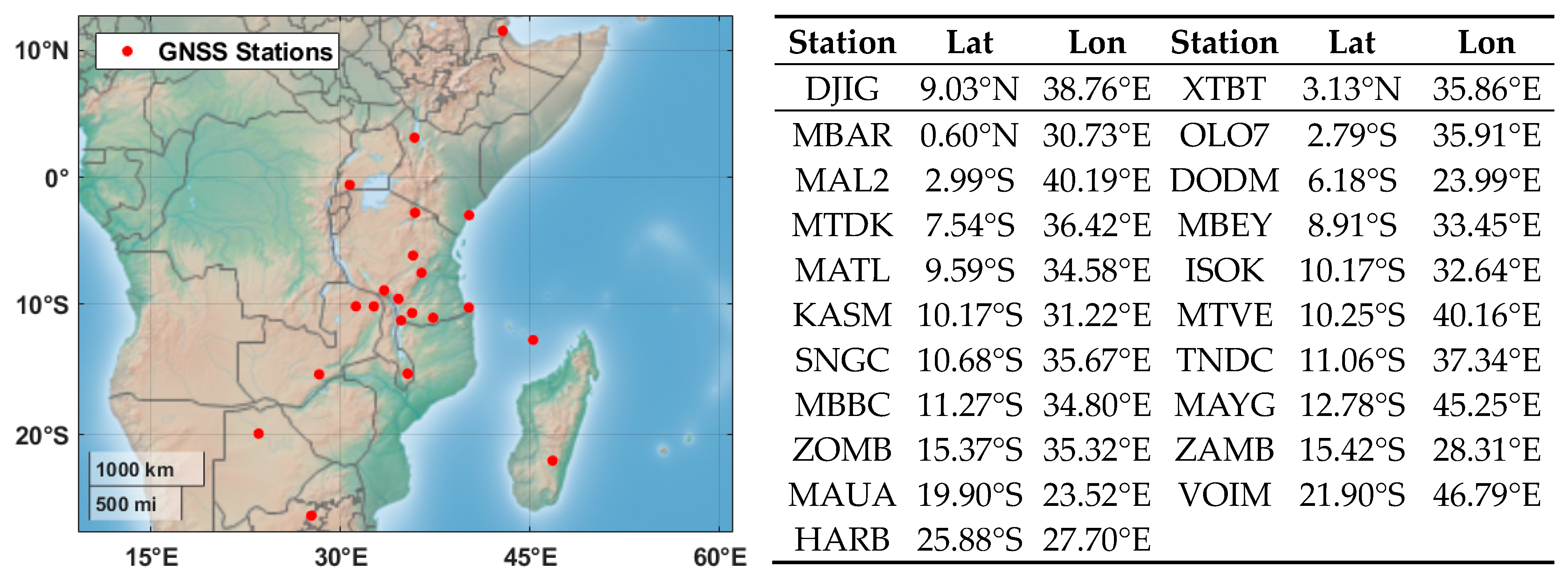
This study involved two primary aspects. Firstly, it entailed an examination of the region and the database of ionospheric parameters derived from 21 ground-based GNSS stations, located within a latitudinal range of 9°N–26°S and a longitudinal range of 24°–47°E over East Africa (where local time LT ≈ UT + 03:00), particularly within the EIA region. This analysis aimed to elucidate ionospheric behavior and its correlations with variations in geophysical parameters during geomagnetic storms. Secondly, the study incorporated observations from the Swarm A and C satellites and the F3/C satellite to discern perturbations in topside ionospheric behavior induced by geomagnetic storms. These satellite observations were then comprehensively compared with ground-based GNSS data and are elaborated upon in the subsequent results and discussion sections. This scientific investigation primarily focused on analyzing ionospheric conditions across different latitudes during the primary phase of a geomagnetic storm.

2. Data Collection

Ionospheric parameters such as TEC and the rate of the TEC index, electron density, and ionospheric scintillation parameters can be used to detect ionospheric perturbations created by geomagnetic storms [10,37]. The slant TEC (STEC) values were measured along the ground-based GNSS signal propagation ray path. The STEC is calculated at a certain height on the ionosphere layer called the ionosphere pierce point (IPP) by measuring satellite motion relative to ground-based GNSS using the intersection of the ray path and the thin-layer ionosphere [38]. Using STEC observations in the line of sight of the satellite, the VTEC parameter can be calculated by dividing STEC by the mapping function $M\left(\epsilon \right)$ as follows:

$$\mathrm{V}\mathrm{T}\mathrm{E}\mathrm{C}=\mathrm{S}\mathrm{T}\mathrm{E}\mathrm{C}/\mathrm{M}\left(\mathsf{\epsilon }\right)$$

(1)

$$\mathrm{M}\left(\mathsf{\epsilon }\right)={[1-{\left(\frac{\mathrm{R}.\mathrm{c}\mathrm{o}\mathrm{s}\left(\mathsf{\epsilon }\right)}{\mathrm{R}+\mathrm{h}}\right)}^2]}^{-1/2}$$

(2)

where $\mathsf{\epsilon }$ represents the elevation angle between the receiver and the satellite, R is the Earth’s radius, and h is the height of the ionospheric layer. In this research, the parameters have been determined at an altitude of 450 km in the ionosphere [39]. It is also possible to provide the rate of TEC (ROT) with high accuracy using differential STEC along the satellite line of sight. The ROT and its standard deviation, known as the rate of TEC index (ROTI), allow for distinguishing the ionospheric irregularities at different scales. The rate of TEC (ROT) unit is TECU/min, where 1 TECU refers to 10¹⁶ electrons/m². The fundamental method for ROT measurement is as follows [40]:

$$\mathrm{R}\mathrm{O}\mathrm{T}=\frac{{\mathrm{S}\mathrm{T}\mathrm{E}\mathrm{C}}_{\mathrm{k}+1}-{\mathrm{S}\mathrm{T}\mathrm{E}\mathrm{C}}_{\mathrm{k}}}{∆\mathrm{t}}$$

(3)

The ROTI measured by the standard deviation of ROT in a time interval is represented as follows [41]:

$$\mathrm{R}\mathrm{O}\mathrm{T}\mathrm{I}=\sqrt{〈{\mathrm{R}\mathrm{O}\mathrm{T}}^2〉-{〈\mathrm{R}\mathrm{O}\mathrm{T}〉}^2}$$

(4)

Previous research such as [41] showed that ROTI is correlated with S4 in different longitude sectors and represents the irregularities with varying scale sizes. In this research, ROTI and S4 were employed to distinguish the occurrence of ionospheric perturbations. The S4, known as the ionospheric amplitude scintillation parameter, is derived from the carrier to noise density (C/N₀) parameter obtained from GNSS receiver observations [42]. The S1 and S2 are used to derive the C/N₀ parameter in two L1 and L2 frequencies from a GNSS observation file. The signal-to-noise ratio (S/N₀) is estimated by C/N₀ as represented in Equation (5). According to Equation (6), the S/N0 detrended (${\mathrm{S}\mathrm{I}}_{\mathrm{d}\mathrm{e}\mathrm{t}\mathrm{r}\mathrm{e}\mathrm{n}\mathrm{d}\mathrm{e}\mathrm{d}}^{\mathrm{S}/{\mathrm{N}}_0}$) can be calculated as follows [43]:

$$S/N_0={10}^{0.1(C/N_0)}$$

(5)

$${\mathrm{S}\mathrm{I}}_{\mathrm{d}\mathrm{e}\mathrm{t}\mathrm{r}\mathrm{e}\mathrm{n}\mathrm{d}\mathrm{e}\mathrm{d}}^{\mathrm{S}/{\mathrm{N}}_0}=\frac{{(S/N_0)}_k}{\sum _{i=1}^{60\times f_s}\frac{{(S/N_0)}_{k-i}}{60\times f_s}}$$

(6)

where C represents the sampling interval and the SI represents the detrended signal intensity measured by signal-to-noise ratio (S/N₀) values. According to Equations (5) and (6), the S4 parameter is obtained from the following equation:

$$S4=\sqrt{\frac{〈{{\mathrm{S}\mathrm{I}}_{\mathrm{d}\mathrm{e}\mathrm{t}\mathrm{r}\mathrm{e}\mathrm{n}\mathrm{d}\mathrm{e}\mathrm{d}}^{\mathrm{S}/{\mathrm{N}}_0}}^2〉-{〈{\mathrm{S}\mathrm{I}}_{\mathrm{d}\mathrm{e}\mathrm{t}\mathrm{r}\mathrm{e}\mathrm{n}\mathrm{d}\mathrm{e}\mathrm{d}}^{\mathrm{S}/{\mathrm{N}}_0}〉}^2}{{〈{\mathrm{S}\mathrm{I}}_{\mathrm{d}\mathrm{e}\mathrm{t}\mathrm{r}\mathrm{e}\mathrm{n}\mathrm{d}\mathrm{e}\mathrm{d}}^{\mathrm{S}/{\mathrm{N}}_0}〉}^2}}$$

(7)

S4 is equal to the standard deviation of the SI in each epoch of interest that is normalized with the average SI of the specified interval and has no unit. S4 and ROTI are used for periods ranging from a few seconds to a few hours. In order to calculate the parameters S4 and ROTI, the average values through five minutes were used [44]. In this research, the S4 and ROTI observations were measured in 5 min intervals by GNSS ground-based observations.

With the two Langmuir plasma probe receivers mounted on the Swarm satellites, electron density values (N_e) can be observed at a rate of 2 Hz [24]. The electron density (N_e) and the rate of electron density index (RODI) can recognize the ionospheric irregularities within the GNSS ground-based region at different scales [45,46]. The fundamental formula for the rate of density (ROD) measurement is as follows:

$$\mathrm{R}\mathrm{O}\mathrm{D}=\frac{{\mathrm{N}\mathrm{e}}_{\mathrm{k}+1}-{\mathrm{N}\mathrm{e}}_{\mathrm{k}}}{∆\mathrm{t}}$$

(8)

The RODI estimated by the standard deviation of ROD in a time interval is represented as follows [47]:

$$\mathrm{R}\mathrm{O}\mathrm{D}\mathrm{I}=\sqrt{〈{\mathrm{R}\mathrm{O}\mathrm{D}}^2〉-{〈\mathrm{R}\mathrm{O}\mathrm{D}〉}^2}$$

(9)

Using the N_e and RODI values obtained from the Swarm mission satellite data, it is possible to detect the electron density behavior and its perturbations during geomagnetic storms at different latitudes and longitudes along the satellite’s flight track. In this research, RODI values were determined in 10 s intervals.

3. Characterizing the September 2017 Geomagnetic Storm

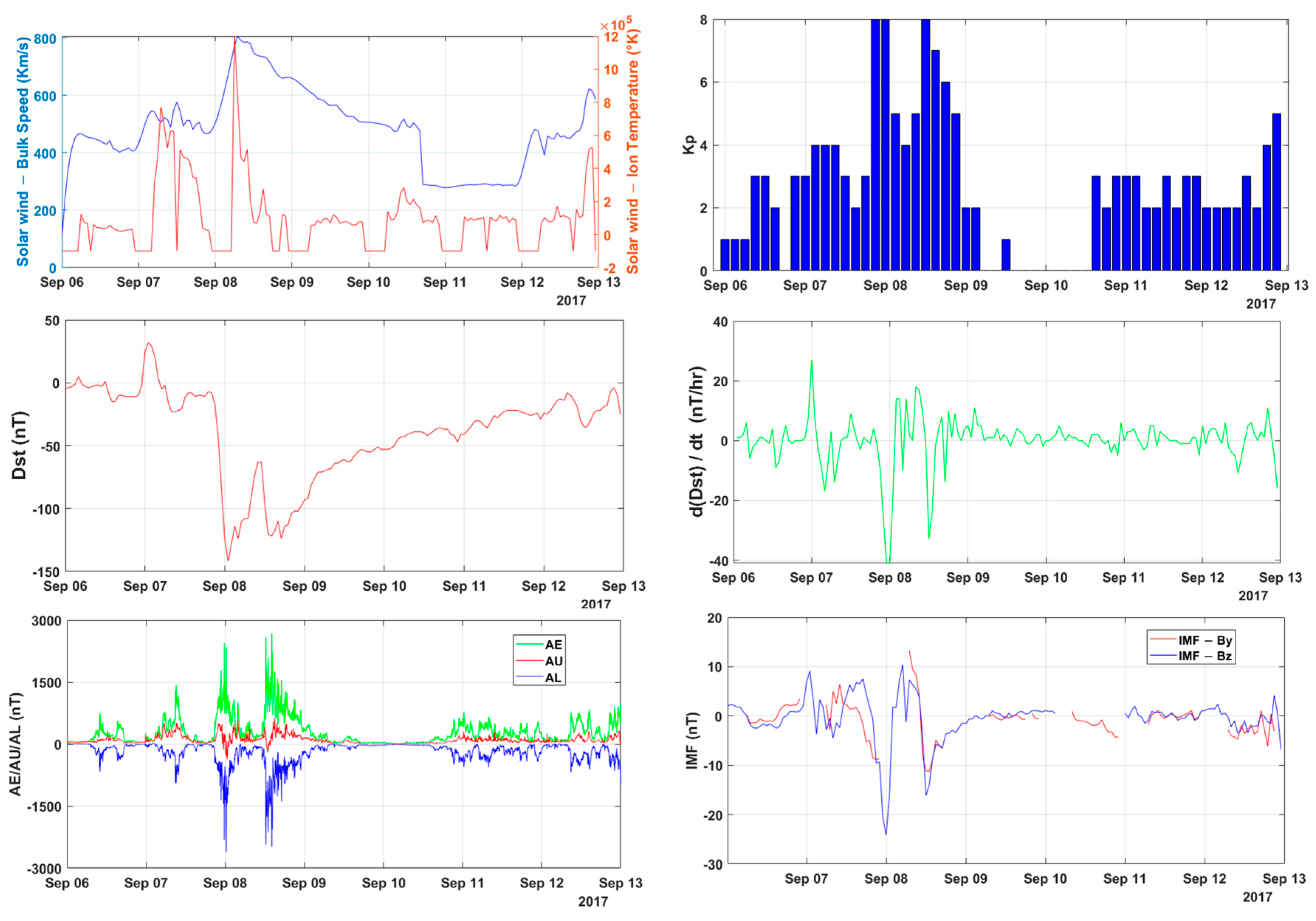
An intense geomagnetic storm occurred 6–12 September 2017 due to solar activity related to a series of coronal mass ejections. The storm’s characteristics are represented in Figure 1 by geophysical data. A set of parameters, such as Dst, AE, d(Dst)/dt (the rate of change of the Dst), and IMF-Bz, were employed to describe the intensity of the geomagnetic storm. Using Figure 1, the most significant disturbance in all geomagnetic parameters occurred during the main phase on 7–8 September 2017. During 10–11 September 2017, the recovery phase of the geomagnetic storm occurred, with disturbances that were much less intense than during than the storm’s main phase.

Investigations into the interplanetary magnetic field (IMF) are pivotal for understanding its influence on geomagnetic storms. The IMF, represented as a three-component vector, was utilized in this study in the geocentric solar ecliptic (GSE) coordinates. The IMF, a vector with three components, holds two components (Bx and By) parallel to the ecliptic plane, while the Bz component is perpendicular to the ecliptic. Disturbances in the solar wind, such as waves and other dynamic phenomena, contribute to the variability in the Bz component. The north–south orientation of the IMF’s Bz component plays a crucial role in determining auroral activity [1]. Examining Figure 1 reveals that the initial intense disturbances occurred abruptly at 23:43 UT on 6 September, with a subsequent severe disturbance transpiring at 23:00 UT on 7 September, collectively identified as SSC. Notably, the IMF-Bz values signify the onset of disturbances with the first SSC, while the most intense perturbations manifested in the concluding hours of 7 September. These significant changes coincided with a rapid southward turning of the IMF-Bz during the main phase of the geomagnetic storm, wherein its value precipitously decreased to −24.2 nT.

The solar wind, a continuous stream of charged particles emanating from the Sun, exhibits variations in its bulk speed and ion temperature, both of which are critical factors influencing space weather. The bulk speed represents the velocity of the solar wind, while the ion temperature reflects the thermal energy of the ions within the solar wind. Variations in these parameters can result in dynamic disturbances in the interplanetary medium, affecting the Earth’s magnetosphere and triggering geomagnetic storms. Understanding the interplay between the bulk speed and ion temperature during the specified period is crucial for unraveling the underlying mechanisms driving the observed geomagnetic phenomena [1]. Figure 1 illustrates the solar wind values concerning two key factors, namely the bulk speed and ion temperature. After the first SSC occurred and in the early hours of 7 September, a notable escalation was discernible in both parameters characterizing the solar wind. After the second SCC event, observed on 8 September a recurrent rising trend was observed, exhibiting a heightened intensity. Remarkably, the peak bulk speed and ion temperature values were documented on 8 September, representing the zenith within the observational timeframe spanning from 6 September to 12 September 12.

The international geomagnetic index Kp is a parameter used to measure the Earth’s geomagnetic activity. The Kp index is employed to evaluate the quiet and disturbed geomagnetic days [48]. A Kp less than three indicates quiet, and a Kp over three represents disturbed geomagnetic conditions [49]. Figure 1 shows that the Kp index suddenly increased in the first and second SSC. After the first SSC occurred, the Kp values took an upward trend, and with the occurrence of the second SSC in the last hours of 7 September, the Kp values reached their maximum with an upward trend.

The Dst index is a magnetic activity index that represents an international equatorial electrojet’s intensity. The Dst index is measured by horizontal geomagnetic observations obtained from networks located near the equator. A negative Dst value means a weaker Earth’s magnetic field and this happens when geomagnetic storms occur [50]. During the first SSC, the Dst and d(Dst)/dt values in the early hours of 7 September first increased and then rapidly took a downward trend. When the second SSC occurred, the Dst suddenly experienced a rapid decline and reached −146 nT, which also caused a sudden change in the trend. The Dst reached its lowest values of −146 nT at 01:00 UT and −115 nT at 13:50 UT on 8 September. The Dst rate experienced two severe rapid drops of −41 nT/h at 23:30 UT and −33 nT/h at 12:00 UT that occurred at about the same time as the two lowest IMF-Bz values.

The auroral electrojet is a fast-flowing current of electrical energy that appears at high latitudes close to the polar regions. The international auroral electrojet (AE) is a parameter used to measure magnetic activity resulting from flowing ion currents in the polar regions. Geomagnetic storms can cause intense auroral electrojets that create disturbances of radio communications and precise navigation [51]. The AE index is measured by AU and AL (AE = AU − AL), with the AU and AL indices representing the maximum and minimum intensity auroral electrojet currents that are observed from horizontal geomagnetic changes above observing stations in the northern hemisphere polar regions [52]. When the first SSC occurred in the last hours of 6 September, the AE experienced an increase and reached 500 nT. The first AE perturbation covering the storm’s main phase started before the second SSC at 20:00 UT on 7 September and continued for nine hours. During this stage, the AE reached 2500 nT at 00:00 UT on 8 September, and the IMF-Bz dropped to its smallest value, −24.2 nT. At 10:50 UT on 8 September, the second AE perturbation occurred and continued to the end of the day. During this stage, the AE reached its peak value of 2677 nT observed on 8 September at 14:06 UT, and the IMF-Bz dropped to its second smallest value, equal to −16.2 nT.

4. Results

This research aimed to analyze the latitudinal effects on the ionospheric perturbations of the main phase of the geomagnetic storm occurring on 6–9 September 2017 through a combination of observations from the network of ground-based GNSS and those of the Swarm and F3/C LEO satellite missions. We employed 21 ground-based GNSS stations in a latitudinal range of 9°N–26°S and longitudinal range 24°–47°E over East Africa (LT ≈ UT + 03:00), located in the EIA, to investigate the ionospheric irregularities’ behavior during geomagnetic storms. The GNSS data received from the network of stations had 15 and 30 s observation rates. The locations of the GNSS stations are shown in Figure 2. The satellite elevation cutoff angle was set to 20 degrees to reduce tracking errors like multipath. In addition to the ground-based GNSS observations, Swarm A and C and F3/C data were taken into account to analyze the ionospheric perturbations during the geomagnetic storm. For this purpose, we used ionospheric data like TEC and S4 from the tangent point between the GNSS and F3/C satellite signal paths near the GNSS ground-based network over Africa. Furthermore, ionospheric electron density data in a 0.5 s interval from the Langmuir plasma probes, as well as ionospheric parameters such as TEC and ROTI from Swarm A and C, were also used in the direction of the Swarm satellites near the GNSS ground stations. Depending on the period and the direction, Swarm A and C can observe one in situ measurement in the daytime and one observation in the nighttime. For this purpose, to evaluate the effect of the geomagnetic storm on ionospheric parameters, GNSS ground-based VTEC average values were measured in one-second intervals. In addition, the average S4 and ROTI values were measured in five-minute intervals by the GNSS stations’ network on 6–9 September.

4.1. Detection of Ionospheric Irregularities Using the Ground-Based GNSS Network

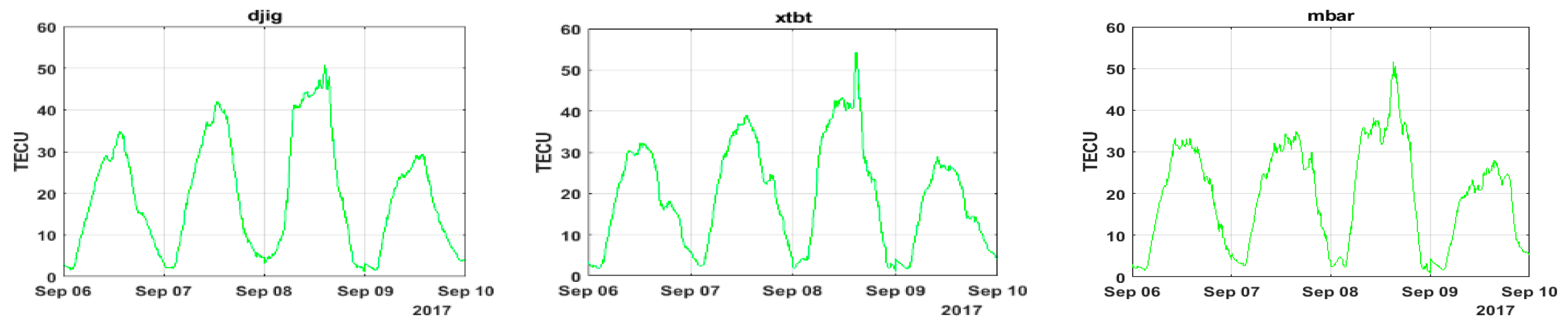
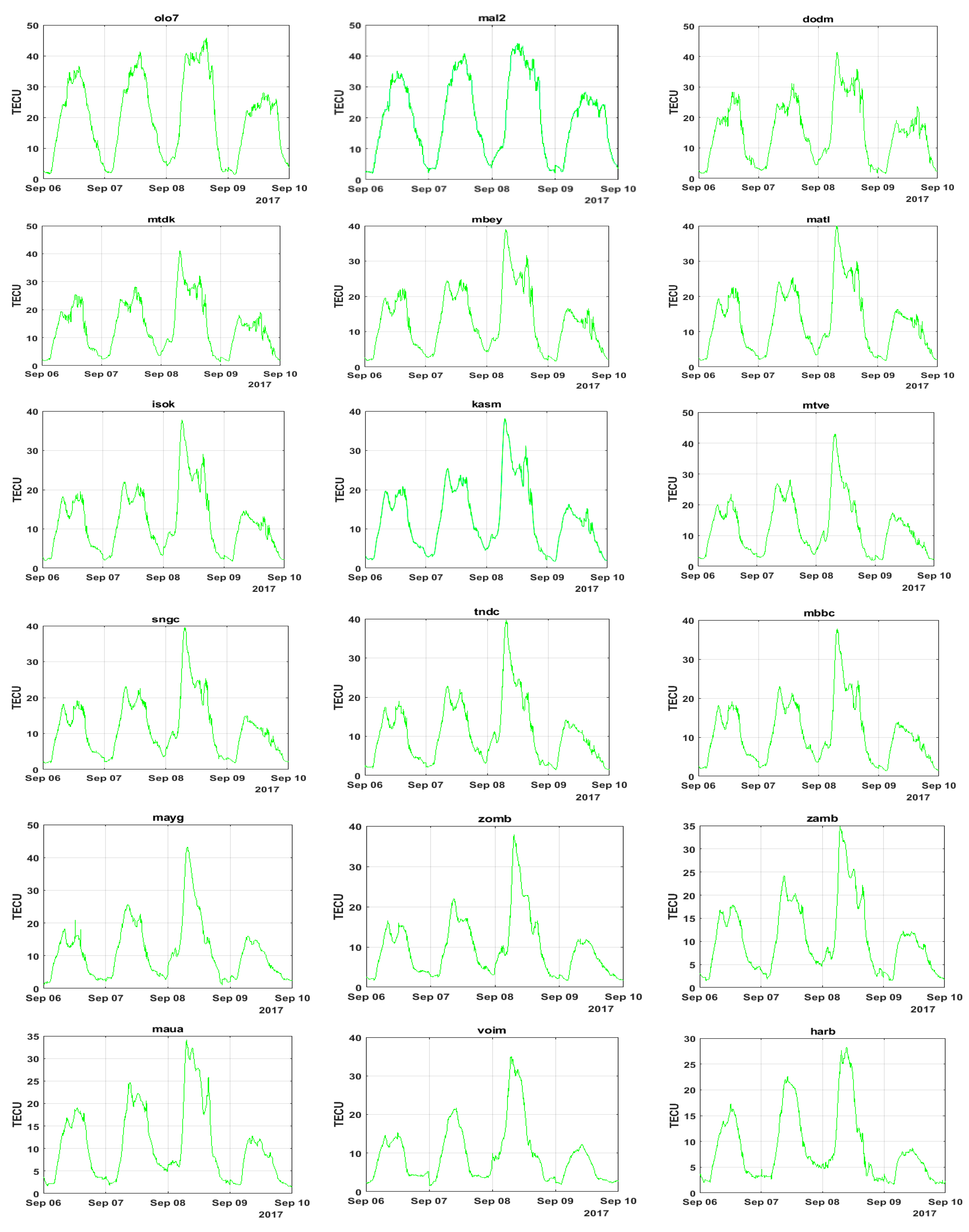
In Figure 3, we present the VTEC data observed by a cluster of GNSS stations situated in the East African region. The arrangement of this dataset, from left to right and top to bottom, corresponds to the latitudinal positions of the individual stations. The primary aim of this analysis was to investigate the latitudinal distribution of the ionospheric irregularities during a geomagnetic storm. A discernible pattern emerged among the northern stations, particularly those proximate to the EIA, such as XTBT, DJIG, and MBAR. These stations exhibited higher VTEC values compared to their southern counterparts, such as HARB, VOIM, and MAUA. This observed behavior aligns with the anticipated ionospheric response near the EIA. To provide context, it is crucial to emphasize the temporal analyses within this dataset. On 6 September, the first SSC event occurred at 23:43 UT, leading to a notable increase in VTEC values across all stations on 7 September. Observations revealed that the VTEC recorded at the DJIG station reached its peak during midday, approximately twice that recorded at the HARB station, which is situated outside the EIA’s range. This disparity underscores the significant spatial variations in the ionospheric electron density distribution.

Subsequently, the more intense second SSC event took place at 23:00 on 7 September, leading to a further rise in the VTEC values on 8 September. The maximum VTEC was recorded on 8 September, marking the peak impact of the geomagnetic storm. This substantial increase underscores the pronounced influence of the storm, particularly near the EIA. The intensity of the VTEC rise gradually diminished in the later hours of 8 September, signaling a transition as the ionospheric conditions began their recovery process. Examining the temporal evolution of the storm, following the subsequent interplanetary shock around 23:00 UT on 7 September, the initial main phase of the storm began. The Dst value reached a minimum of −142 nT at 01:00 UT on 8 September, with the solar wind and Kp indices indicating a severe geomagnetic storm. The solar wind parameters, Dst, and Kp indices gradually recovered until the end of 8 September. In parallel, the AE index peaked at 1157 nT during the first main phase of the storm at 23:00 UT.

Throughout the main phase of the geomagnetic storm, there was a slight enhancement in VTEC. Additional contributions to the rise in VTEC came from flares in the IMF-Bz component at 23:50 UT on 7 September and a sudden burst in AE, leading to a rapid increase in VTEC during the early hours of 8 September. This heightened VTEC persisted until approximately 07:00 UT on 8 September, after which a negative ionospheric storm commenced, characterized by a sharp increase in VTEC around 12:00 UT on 8 September, extending into the second main phase of the storm. Furthermore, a sharp southward turn in the IMF Bz component occurred at approximately 12:00 UT on 8 September, heralding the onset of the second main phase of the storm, characterized by a minimum Dst value of −124 nT at 17 UT on 8 September. By 9 September, the mean VTEC values had reached their lowest point, marking the end of the storm’s acute effects. During the recovery phase, the VTEC exhibited a sharp decrease on 9 September. In addition to analyzing the VTEC, it is crucial to explore the broader impact of the geomagnetic perturbations on the ionospheric activity from 6 September to 9 September. This comprehensive assessment involved examining parameters such as S4 and the ROTI, providing insights into ionospheric irregularities induced by geomagnetic disturbances. This multifaceted approach enabled a more nuanced understanding of the intricate interplay between the geomagnetic storm and the ionosphere within this group of GNSS stations.

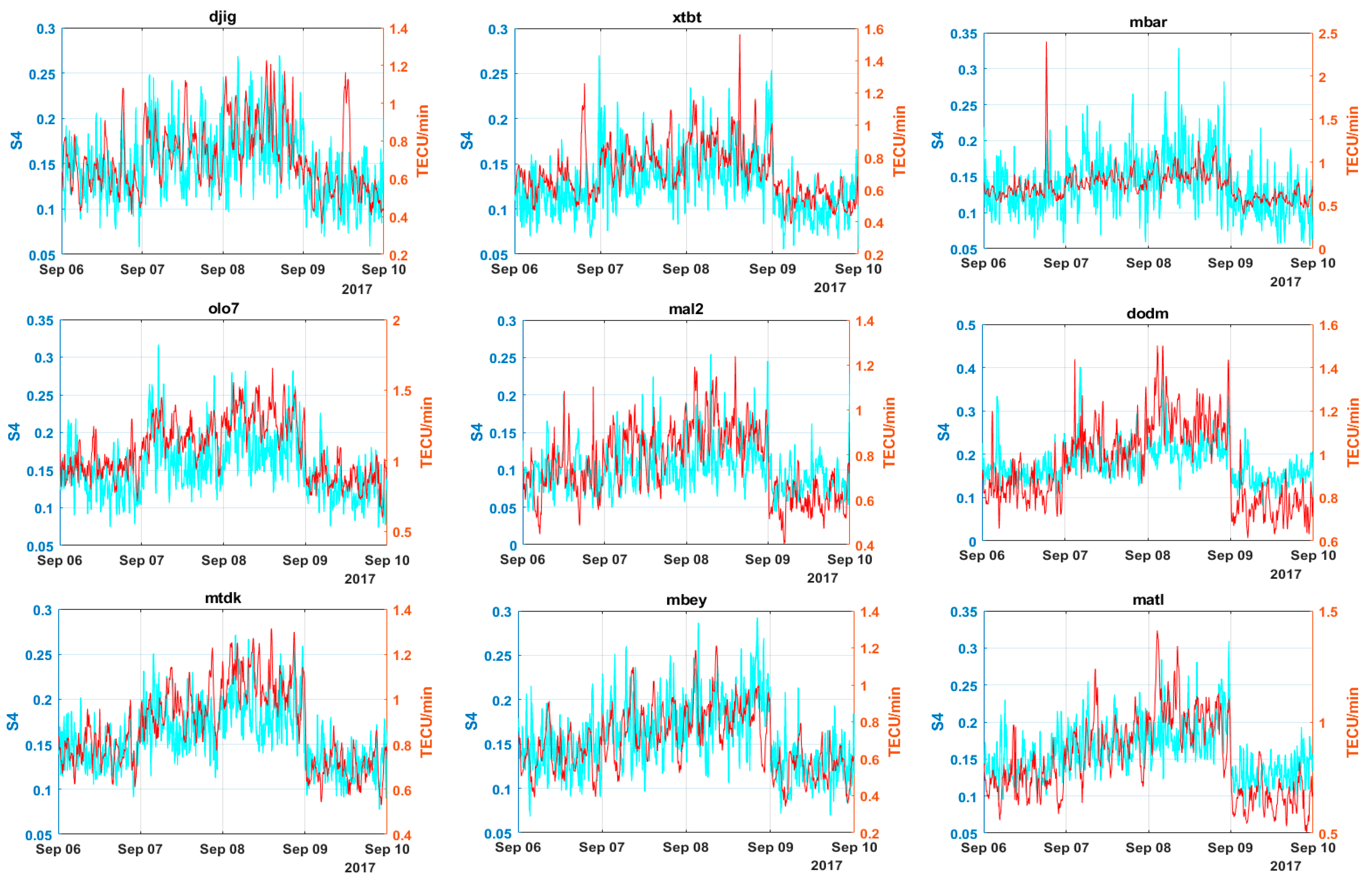
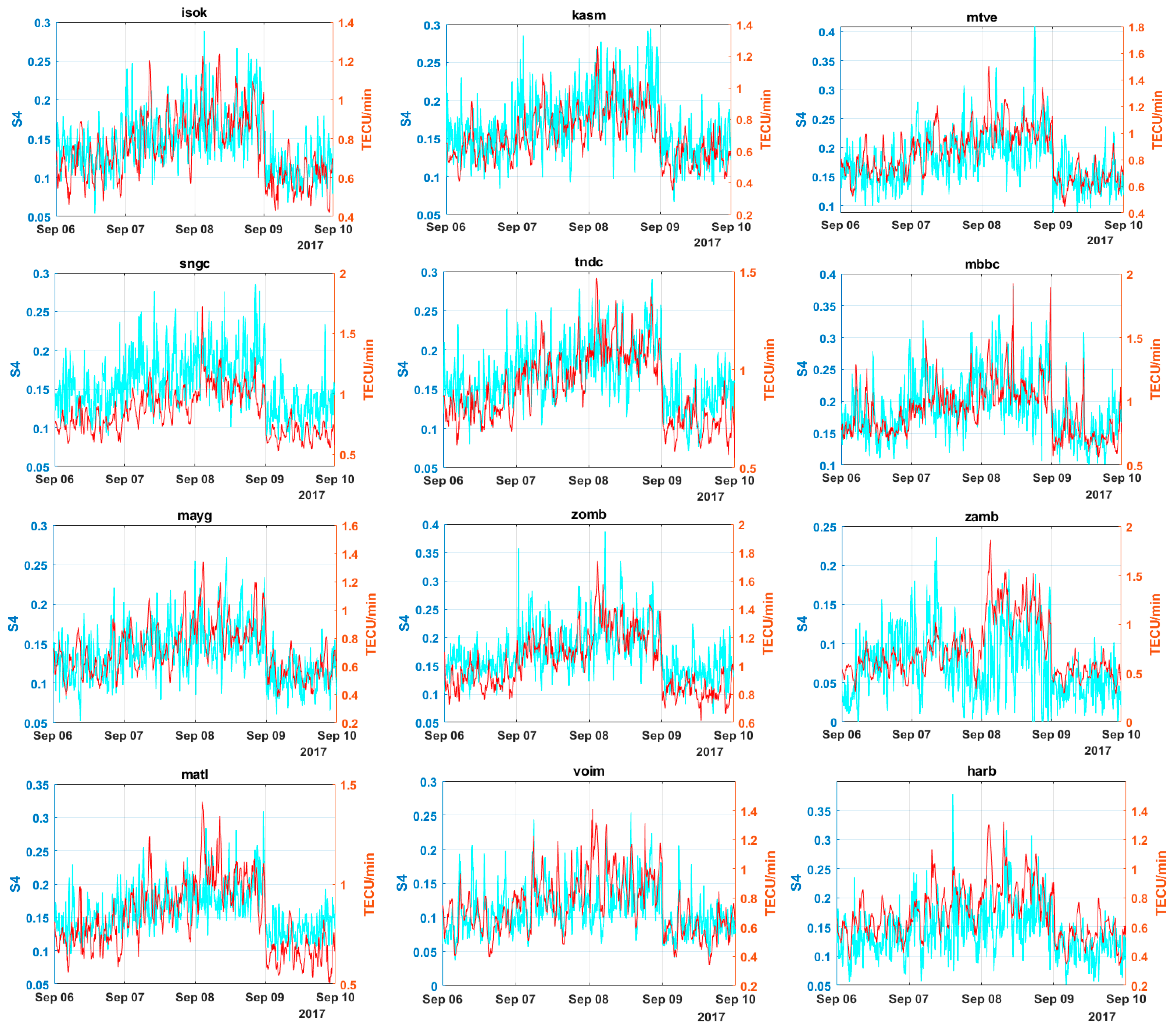
Figure 4 portrays a time-series analysis of ionospheric scintillation parameters, S4 and ROTI, extracted from the GNSS ground-based stations. These parameters hold significance in characterizing ionospheric irregularities, with S4 values exceeding 0.2 indicating scintillation events [44]. Upon initial examination of the S4 and ROTI observations, a discernible correlation between these two parameters becomes apparent. Moreover, referring to Figure 4, it becomes evident that the observations over a four-day period exhibited an upward trending arc, indicating an upward trend in both the ROTI and S4 on 7 September and 8 September. Stations in close proximity to the EIA, such as DJIG and XTBT, experienced a sudden increase in S4 during the late hours of 6 September and early hours of 7 September, also observable in the ROTI, though with less pronounced intensity. Intermediate stations like MTDK and ISOK similarly witnessed an upsurge in S4 during the late hours of 6 September, accompanied by a corresponding increase in ROTI values, suggesting a concurrent upward trend during this timeframe. On 6 September, the southern stations exhibited no significant fluctuations in S4 or the ROTI during the first SSC, aligning with the expected behavior. On this day, S4 values rarely exceeded 0.2, indicating a lack of noteworthy ionospheric scintillation, with some stations showing brief periods of S4 exceeding 0.2, potentially due to local and transient events. Following the first SSC on 7 September, a noticeable increase in S4 and ROTI occurred across all stations. Stations within the EIA region, such as OLO7 and XTBT, experienced ionospheric scintillation during the early hours of 7 September. MBAR recorded intermittent scintillation events throughout the day. A comparison with the values from the preceding day highlights the impact of the initial phase of the geomagnetic storm on the emergence of ionospheric irregularities within the EIA region.

The consequences of the more intense second SSC were evident across all stations, with the highest levels of S4 and the ROTI recorded on this day. The mean values of S4 and the ROTI also showed a significant increase compared to 7 September. Around the time of the second SSC, observed in the late hours of 7 September near the EIA region, the onset of ionospheric irregularities was apparent. Stations like DJIG, DODM, and MTDK observed scintillation in the early hours of 8 September. As shown by S4, EIA stations like MBAR and DJIG experienced ionospheric disturbances throughout most of the day, with the ROTI values exhibiting a significant increase. Intermediate stations also exhibited ionospheric scintillation, at times more intensely observed in northern stations in the central EIA area. This heightened intensity may be attributed to the Rayleigh–Taylor process, bringing ionospheric plasma bubbles into the southern regions of the EIA, leading to increased ionospheric irregularities. With the initiation of the PPEF process, southern stations likewise observed an increase in S4 and the ROTI, resulting in scintillation in the southern regions. Toward the end of 8 September and the onset of the DDEF process, a sharp decline in both S4 and the ROTI was observed, resulting in lower mean values compared to the observations on 6 September. Stations within the EIA region experienced a more pronounced decrease, particularly evident at stations XTBT, OLO7, and DODM. This sharp drop commenced in the late hours of 8 September and reached its peak on 9 September. On 9 September, S4 revealed the absence of ionospheric disturbances across all stations, which was particularly prominent in stations in the middle and southern regions. These outcomes can be attributed to the lowering of the F layer height and the reduced incidence of ionospheric plasma bubbles, resulting from the initiation of the DDEF process in the ionosphere. This comprehensive analysis provides insights into the behavior of ionospheric irregularities using the TEC, ROTI, and S4 observations over a four-day time series during a geomagnetic storm, along with the subsequent ionospheric behavior, utilizing GNSS ground-based stations in East Africa.

4.2. Influences of Ionospheric Irregularities on Swarm Observations

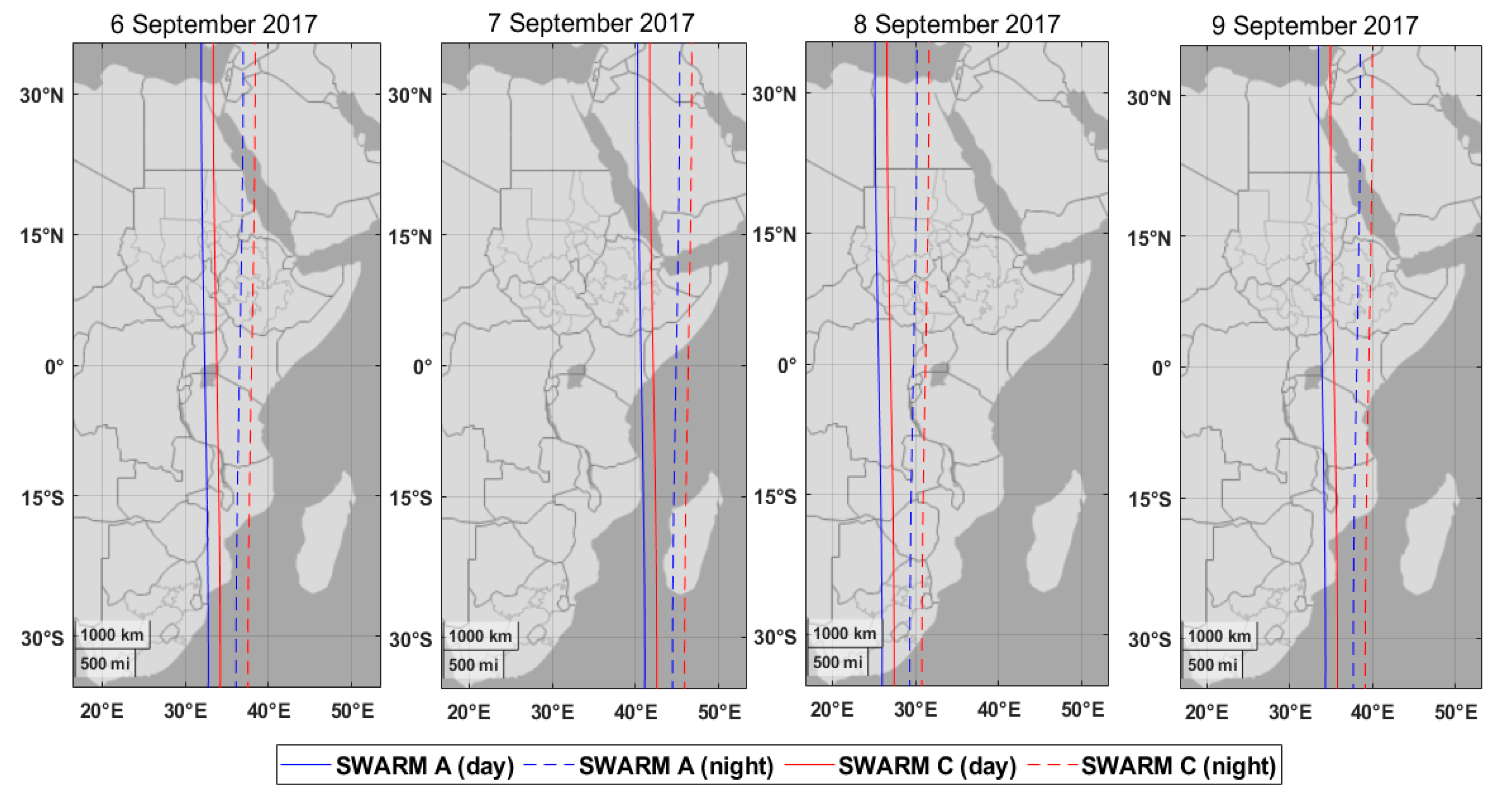
In this study, we explored the influences of geomagnetic storms on ionospheric parameters from 6–9 September 2017, utilizing observations from both ground-based GNSS stations and Swarm A and C satellites. The orbital paths of Swarm A and C satellites near three GNSS ground-based stations and over Africa during both daytime and nighttime are depicted in Figure 5. The Langmuir probe on the Swarm A and C satellites provided in situ density data during orbits over the African region, crucial for our investigation. We set the elevation cutoff angle to 30° in this study. Swarm A and C observations included ionospheric parameters such as the VTEC, ROTI, Ne, and RODI. It is noteworthy that these parameters exhibited lower values compared to the ground-based GNSS measurements due to the altitude disparity between the GNSS stations and the Swarm satellites. While ground-based GNSS observations covered the entire ionosphere along the slant paths, the Swarm A and C satellites, situated 450 km above the ground, provided a limb viewing path. Consequently, a discrepancy in values between the Swarm A and C and GNSS ground-based observations was anticipated. The ionospheric parameters obtained from Swarm A and C contribute to understanding the effects of the geomagnetic perturbations on the upper ionosphere. 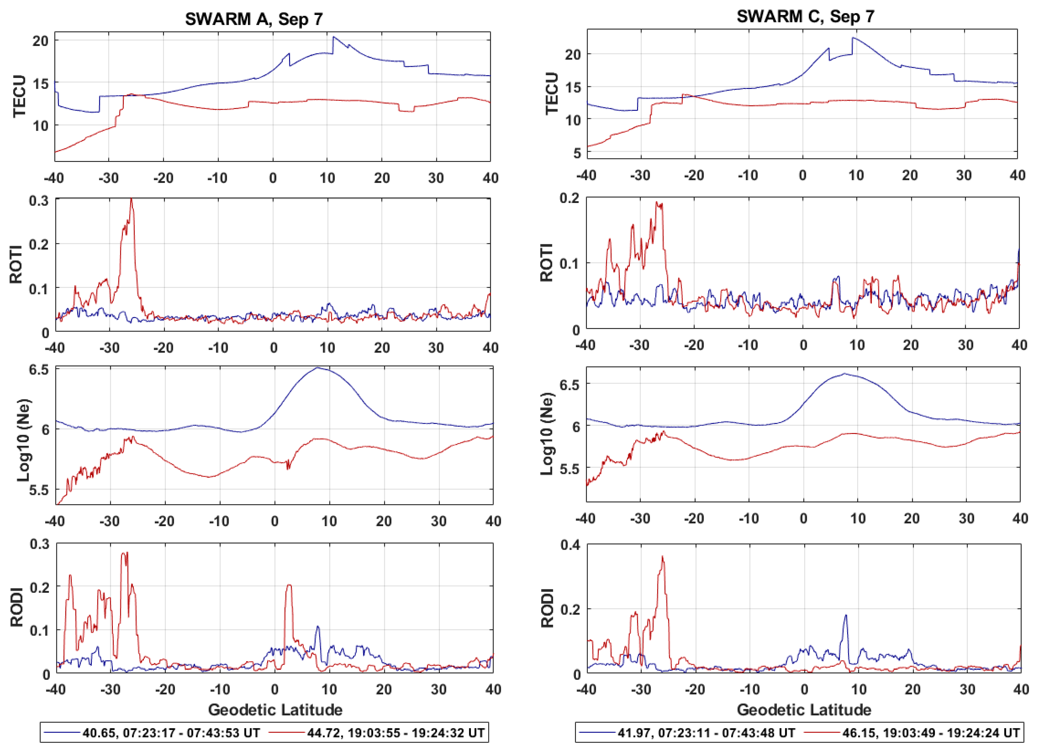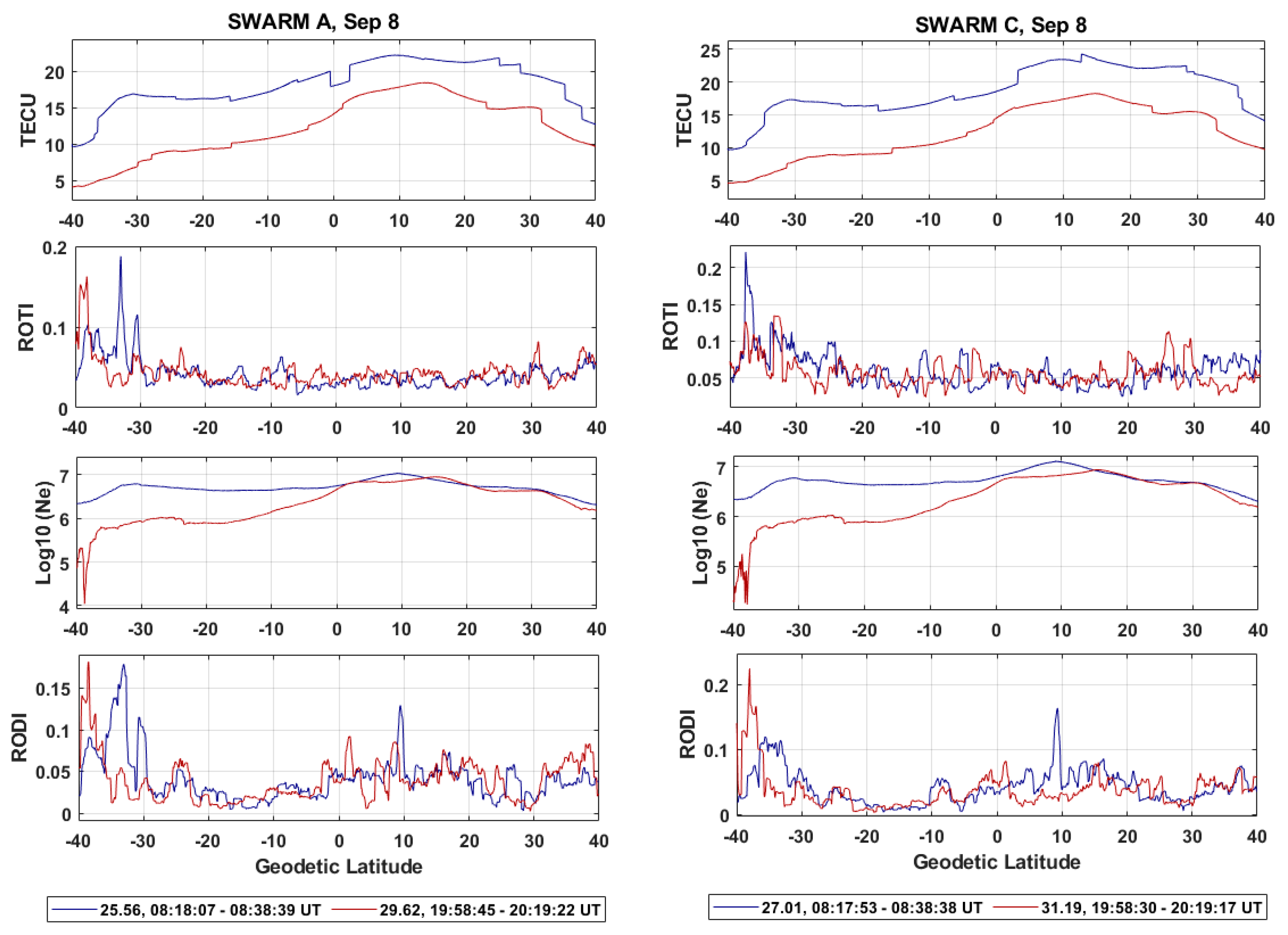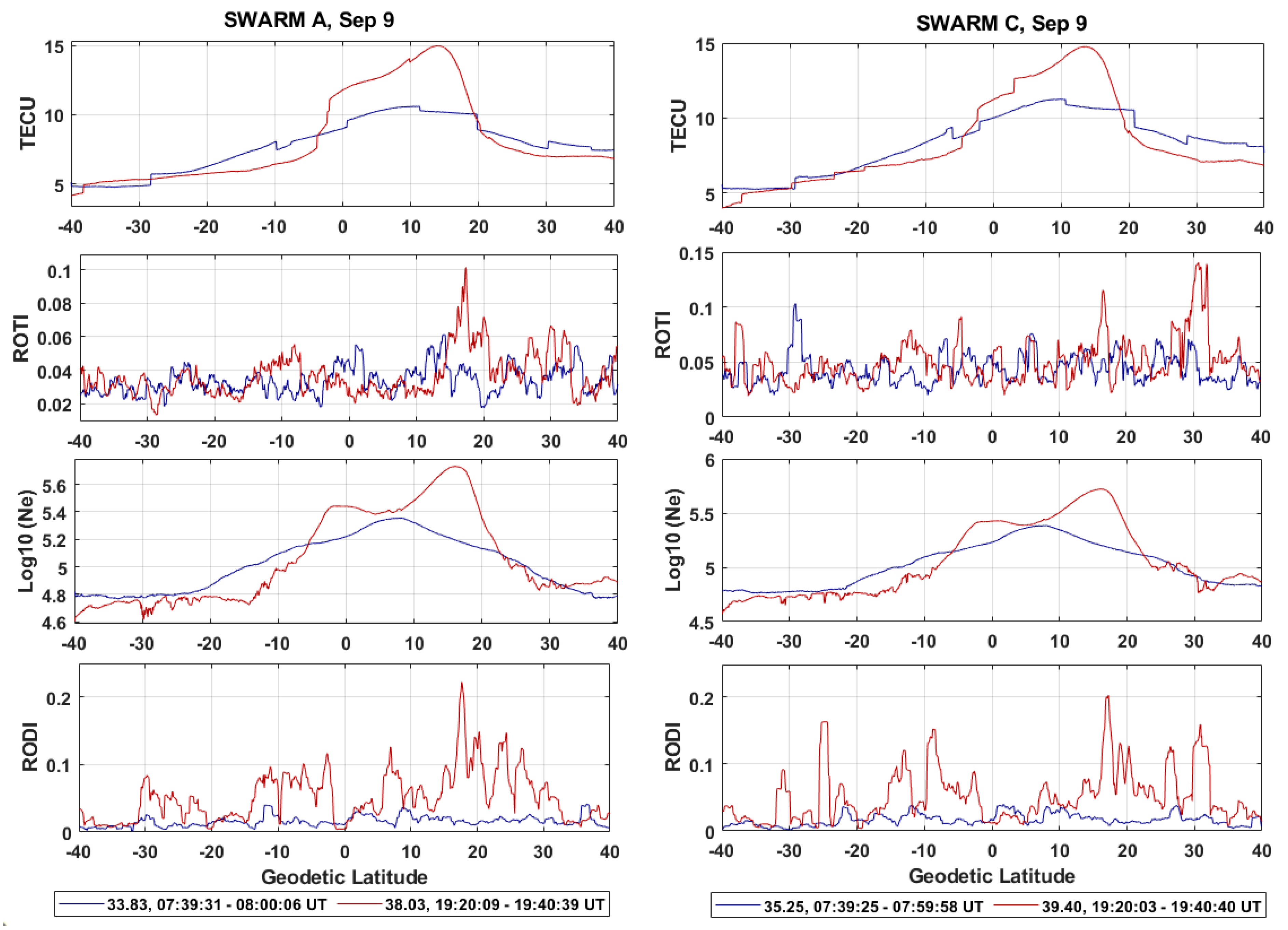Figure 5, Figure 6, Figure 7 and Figure 8 illustrate the impact of the geomagnetic perturbations on the VTEC, Ne, ROTI, and RODI values within latitudes from −40° to +40° and longitudes near the GNSS stations during intervals of day and night from 6 to 9 September 2017.

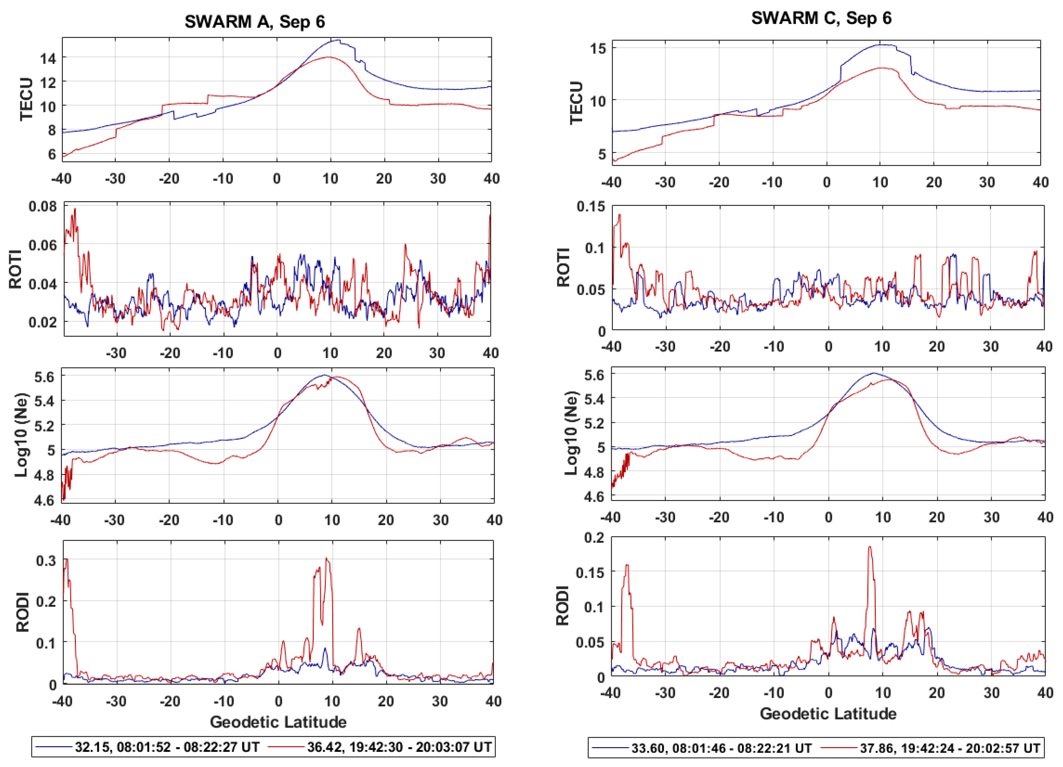
Examining Figure 6, we observe that the VTEC and Ne values exhibited a similar trend during both daytime and nighttime on 6 September. Notably, the highest values occurred near the equator. The mean VTEC values for Swarm A and C during daytime and nighttime were closely aligned, differing by less than 0.5 TECU. Conversely, the ground-based GNSS VTEC values increased during nighttime, and the Ne values displayed a similar trend. The rapid increase in Swarm A and C VTEC at nighttime, especially as the satellites moved from northern latitudes toward the equator before the first SSC event, is indicative of the heightened geomagnetic parameters. This increase is evident in disturbance parameters like the ROTI, peaking at nighttime between −30° and −40°. The RODI, representing disturbances in electron density, experienced a sudden increase, particularly in the geographical latitude intervals (−30°, −40°) and (0°, 10°) during nighttime on Swarm A and C.

On 7 September, the observed VTEC and Ne values increased compared to the previous day. The elevation in ionospheric disturbance parameters, which ensued following the occurrence of the first SSC in the late hours of 6 September, was followed by the initiation of the initial phase of the geomagnetic storm on 7 September. The mean VTEC values for Swarm A and C on this day rose by nearly 5 TECU (Figure 7). Notably, electron density disturbances were more prevalent in southern latitudes, as indicated by the increased RODI values in this region. The second SSC event, occurring in the last hours of 7 September, contributed to the rise in ROTI values in the southern latitudes. On 8 September, we witnessed the highest measured VTEC values during the four days, particularly during the daytime (Figure 8). The second SSC incident enhanced the ROTI values in the southern latitudes, with the most severe disturbances observed during both day and night. Despite a reduction in the severity of geomagnetic disturbances in the late hours of 8 September, the VTEC values increased slightly compared to the previous night. Swarm A and Swarm C both exhibited an increase in the Ne throughout the day and night, with the highest values observed near the equatorial regions. Disturbances, as indicated by the ROTI and RODI measurements, were most pronounced in the southern range during both day and night.

As geomagnetic disturbances waned in the final hours of 8 September, the mean VTEC values on 9 September decreased significantly compared to the previous day. Notably, the nighttime observations on 9 September displayed higher values than the daytime observations, signaling the onset of the ionospheric recovery process. The increase in VTEC was more pronounced near the equator, possibly influenced by the behavior of the EIA. Unlike the primary phase of the geomagnetic storm, where disturbances were more prominent in the southern latitudes, the recovery phase exhibited intensified disturbances near the EIA during the night. Similar trends were observed in the ROTI and RODI values on 9 September at night. The mean values of VTEC and Ne during both the daytime and overnight intervals were decreased compared to the previous day, indicating a less intense recovery phase of the geomagnetic storm (Figure 9).

Table 1. The VTEC, ROTI, Ne, and ROTI values of Swarm A near the GNSS ground-based stations 6–9 September 2017.

Swarm A	Mean TEC	Max TEC	Mean ROTI	Max ROTI	Mean Log10 (Ne)	Max Log10 (Ne)	Mean RODI	Max RODI
6 September (day)	10.71	15.46	0.03	0.05	5.14	5.60	0.01	0.08
6 September (night)	10.25	14.01	0.03	0.07	5.08	5.58	0.04	0.30
7 September (day)	15.56	20.37	0.04	0.06	6.62	7.07	0.03	0.10
7 September (night)	11.95	13.61	0.05	0.31	6.26	6.45	0.04	0.27
8 September (day)	18.19	22.26	0.05	0.18	6.71	7.03	0.04	0.17
8 September (night)	12.21	18.47	0.05	0.16	6.33	6.95	0.03	0.18
9 September (day)	7.76	10.60	0.03	0.06	5.01	5.35	0.01	0.04
9 September (night)	8.19	14.97	0.03	0.10	5.05	5.72	0.05	0.22

and

Table 2. The VTEC, ROTI, Ne, and ROTI values of Swarm C near the GNSS ground-based stations 6–9 September 2017.

Swarm C	Mean TEC	Max TEC	Mean ROTI	Max ROTI	Mean Log10 (Ne)	Max Log10 (Ne)	Mean RODI	Max RODI
6 September (day)	10.41	15.25	0.03	0.09	5.15	5.60	0.01	0.07
6 September (night)	9.94	13.05	0.04	0.13	5.07	5.54	0.02	0.18
7 September (day)	15.76	22.94	0.04	0.12	6.67	7.19	0.02	0.18
7 September (night)	11.75	13.81	0.05	0.19	6.25	6.45	0.03	0.36
8 September (day)	18.67	24.29	0.06	0.22	6.72	7.11	0.04	0.16
8 September (night)	12.24	18.25	0.05	0.13	6.32	6.94	0.03	0.22
9 September (day)	8.35	11.26	0.04	0.10	5.02	5.38	0.01	0.03
9 September (night)	8.41	14.76	0.05	0.14	5.05	5.72	0.05	0.20

present the observational values for these four days obtained from the Swarm A and Swarm C satellites.

4.3. Signatures of Ionospheric Irregularities in the FORMOSAT3/COSMIC (F3/C) Observations

In this study, alongside the ground-based GNSS networks in East Africa and the Swarm A and C satellite data, we incorporated ionospheric irregularity measurements from radio occultation (RO) observations obtained by FORMOSAT3/COSMIC (F3/C). These observations, taken at the tangent point between the GNSS and F3/C satellites, contribute to understanding the impact of geomagnetic storms on ionospheric parameters 6–9 September 2017. Parameters such as the VTEC and S4 were derived from the F3/C observations. It is crucial to note that the F3/C ionospheric parameters exhibited lower values compared to the ground-based GNSS measurements. This discrepancy arises from the transformation of inclined RO observations into vertical ones, taking place at an altitude of 200 to 400 km above the ground (the limb viewing path). In contrast, the GNSS observations cover the entire column of the ionosphere. Thus, the expected difference in values between these two observation methods is a result of their distinct measurement perspectives [30]. Variations in ionospheric characteristics, as measured by F3/C, offer insights into the pattern of geomagnetic storm impacts on the upper ionosphere. 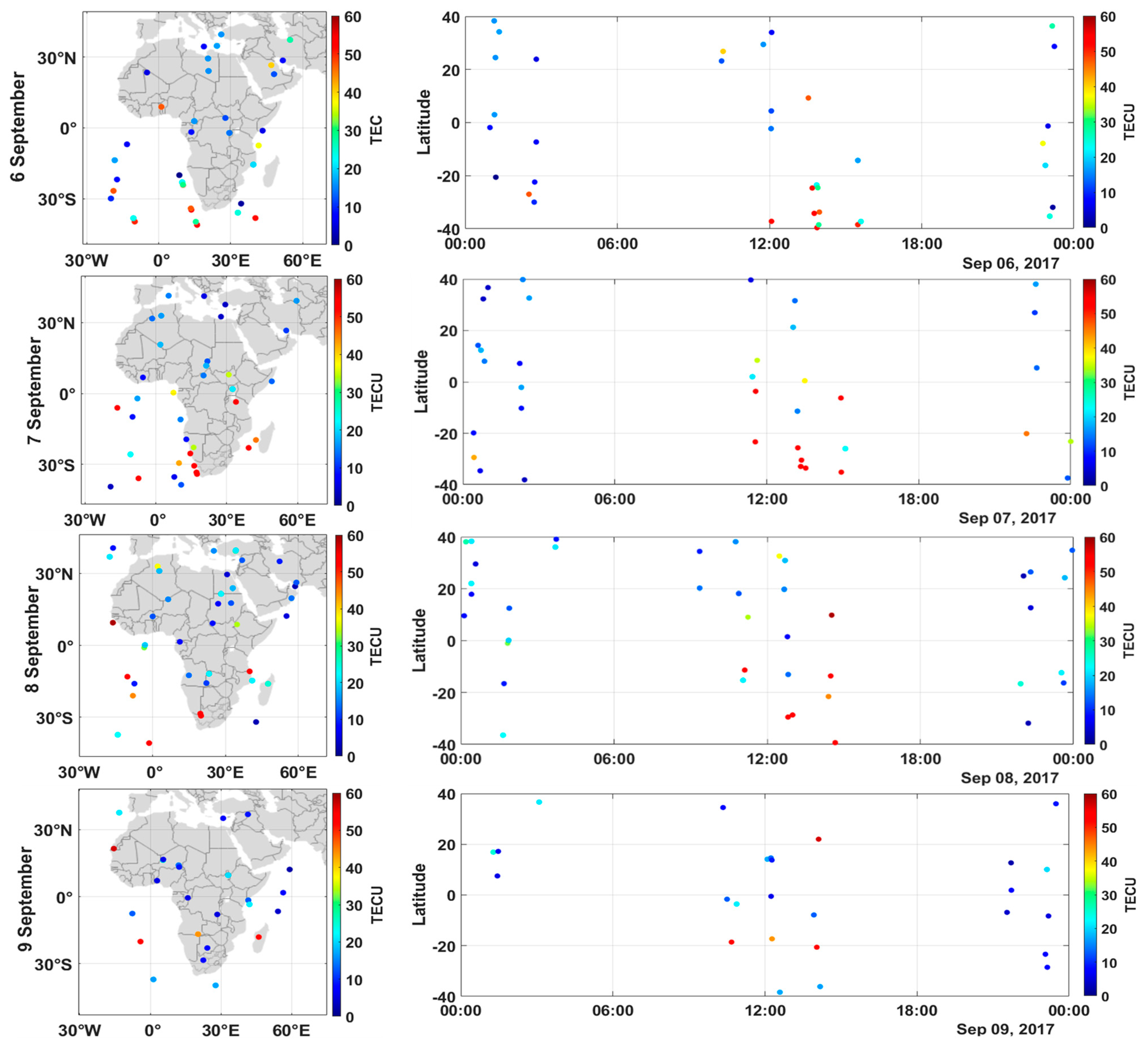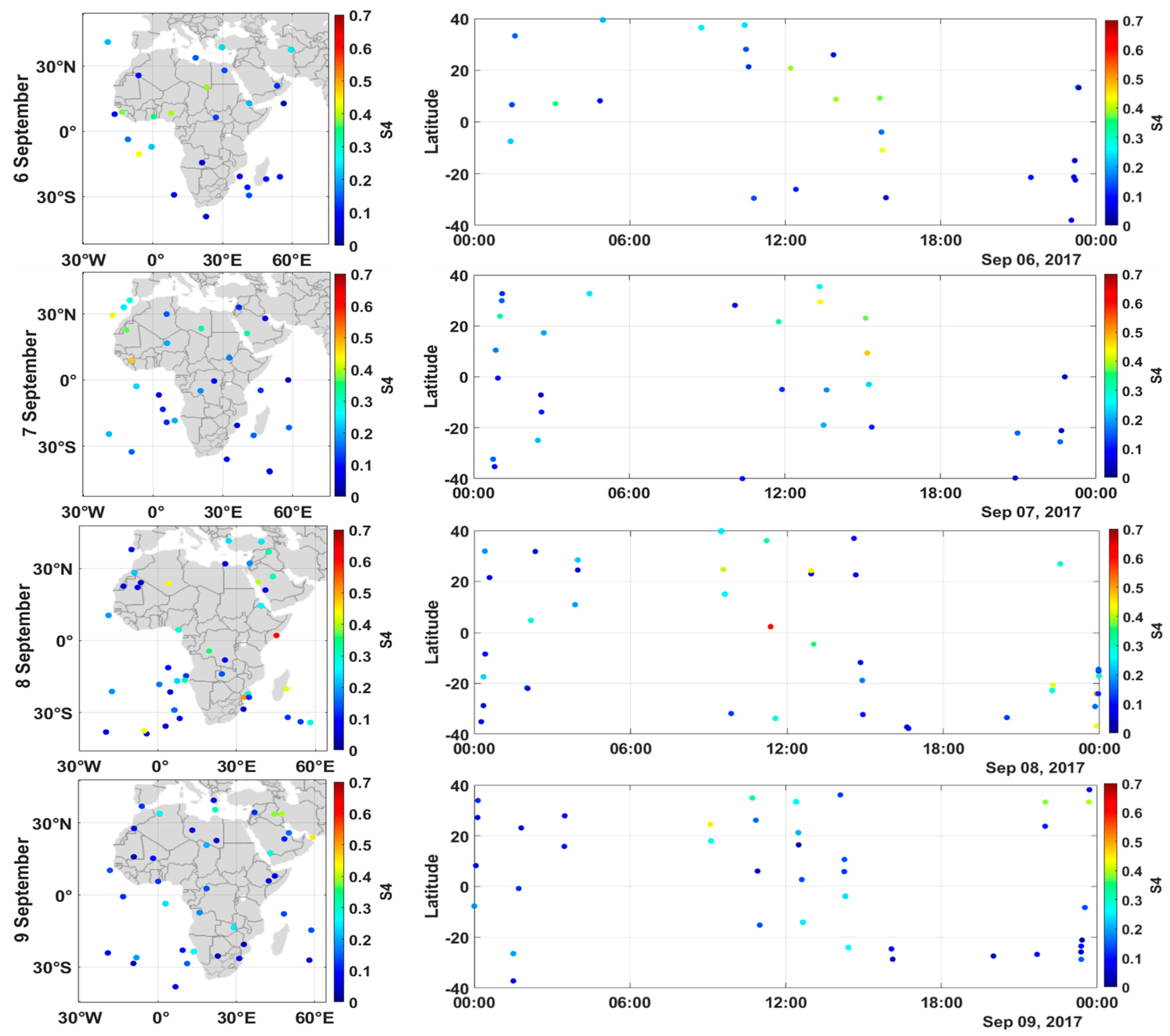Figure 10 and Figure 11 depict the 24 h distribution of the F3/C radio occultation data over Africa within latitudes −40° to +40° and longitudes −20° to +60° 6–9 September 2017. Approximately 40 occultation occurrences per day were recorded for all GNSS satellites near the ground-based GNSS networks and across Africa.

Figure 10 presents the VTEC and S4 values acquired from the RO data for the four study days. The maximum VTEC values from F3/C occurred around mid-day (UT), mirroring the VTEC trends observed in the ground-based GNSS measurements. Following the first SSC event in the late hours of 6 September, the F3/C VTEC values increased, with a noticeable upward trend on 7 September. The daily average VTEC on 7 September increased by 2.65 TECU compared to the previous day, reaching 25.03 TECU. The second SSC event at 23:00 on 7 September further increased the VTEC on 8 September, with the maximum mean VTEC values observed on this day. The ionosphere began recovery in the late hours of 8 September, resulting in the lowest mean VTEC on 9 September at 19.62 TECU.

The S4 values, representing ionospheric amplitude scintillation, increased after the first SSC occurrence in the final hours of 6 September. Mean S4 values rose from 0.19 to 0.21 on 7 September, indicating the effects of geomagnetic perturbations. On 8 September, the daily average of ionospheric scintillation climbed to 0.23, indicating sustained scintillation throughout most of the day. The peak ionospheric scintillation values occurred around mid-day (UT) on 8 September near the EIA. The highest S4 value recorded during the four days was 0.60. With the decline in geomagnetic activity in the late hours of 8 September and the commencement of 9 September, the daily mean of S4 decreased dramatically, similar to the VTEC pattern, dropping to 0.16, signifying a reduction in the strength of the geomagnetic disturbances.

Table 3. The VTEC and S4 values of F3/C near the GNSS stations over Africa 6–9 September 2017.

Date	Mean VTEC	Max VTEC	Mean S4	Max S4
6 September	22.38	53.97	0.19	0.49
7 September	25.03	54.66	0.21	0.53
8 September	26.33	58.64	0.23	0.60
9 September	19.62	53.61	0.16	0.44

presents observational values for these four days obtained from F3/C.

5. Discussion

In the context of this study, a thorough examination of ionospheric conditions at diverse latitudes during the initial stage of a geomagnetic storm has been undertaken. The ensuing analysis offers an extensive evaluation of ionospheric conditions spanning both low latitudes and the EIA throughout the geomagnetic storm that transpired. The enhancement in the TEC during the geomagnetic storm is attributed to undershielding conditions resulting from a negative IMB-Bz, which led to the prompt penetration of electric fields from the magnetosphere into the equatorial ionosphere. The undershielding PPEF superimposed itself on the pre-existing equatorial zonal electric fields, consequently modifying the regular pattern of ionospheric dynamics and electrodynamics. In line with fundamental ionospheric electrodynamics principles, the undershielding PPEF exhibited an eastward orientation during the daytime, which, in turn, amplified the vertical E×B drift [53]. A substantial amount of plasma was transported upward near the magnetic equator as a result of the intensification of the fountain effect. Subsequently, this plasma diffused through the magnetic field lines toward higher latitudes. The loss rate of plasma decreases with altitude more rapidly than the production rate, which enables this transport process to increase the ionization density in the topside ionosphere more efficiently [54].

Confirmation of the presence of a PPEF hinges on the measurement of electric fields. However, when such data are unavailable, alternative reliable indicators come into play. Sudden fluctuations, whether increases or decreases, in the AE index and corresponding abrupt shifts in the Dst index provide valuable insights into the strength, polarity, and timing of electric field penetration across equatorial and low-latitude regions [55,56]. Additionally, previous research has effectively used the rate of change of the Dst index (Dst/dt) as a proxy for this purpose [57,58].

In Figure 1, a notable surge in the AE index from 1400 to 2400 nT is observed, coinciding with a rapid decrease in the Dst/dt (approximately 41 nT per hour) at around 2330 UT on 7 September. These observations suggest that the southward shift of the IMF-Bz, reaching a minimum value of approximately −30 nT, established an undershielding condition, leading to the emergence of a PPEF in low-latitude regions at approximately 23:30 UT. PPEFs are instantly associated with the southward turning of the IMF-Bz and typically last for a short period of time, approximately one to two hours. As a result, PPEFs can persist for much longer periods of time under prolonged southward IMF-Bz periods, up to 8–10 h [59]. Importantly, PPEFs exhibit an eastward polarity during the day and a westward polarity during the night.

The VTEC values exhibited a significant reduction at the conclusion of the main phase and the commencement of the recovery phase, which is discernible from the ROTI and S4 values around 9 September. The general upsurge in VTEC was primarily related to the prolonged presence of eastward PPEFs, which exacerbated the typical equatorial daytime E×B drifts for several early hours [59]. This phenomenon aligned with the southward shift of the IMF-Bz, with a magnitude less than −20 nT (Figure 1), at the beginning of the main phase of the geomagnetic storm. The AE index, which is directly related to Joule heating (JH), is governed by the equation JH = 0.33 AE [60], where JH is expressed in nT. As a result of the storm’s initial main phase, the AE index (Figure 1) exhibited a substantial increase, reaching a maximum value of 1157 nT, signifying a high-latitude JH responsible for generating storm-induced thermospheric currents that, in turn, produced DDEFs [61]. Notably, DDEFs have a different polarity than PPEFs and emerge subsequent to PPEFs, with timescales ranging in length from minutes to hours, and are dominant during the storm recovery phase. A sustained decline in the VTEC over the latter part of the recovery phase on 8 September can be attributed to changes in the storm-time equatorial ionosphere electrodynamics and structural alterations linked to storm-induced high-latitude gas circulation featuring a depleted O/N₂ density ratio transported to lower latitudes due to auroral JH effects [62]. The recovery phase, caused by the southward shift of the IMF-Bz, was initiated on 8 September, with a minimum DST index reaching −124 nT at 17:00 UT on 8 September. The decline in the VTEC, which commenced near the end of the main phase and extended throughout most of the recovery phase, underscores the dominant influence of DDEFs in the main phase on PPEFs in the recovery phase. The AE index (Figure 1) exhibited a sharp increase during the main phase, peaking at 1442 nT around 14 UT on 8 September, signifying a robust high-latitude JH responsible for generating DDEFs [4]. The VTEC data demonstrated a pronounced positive ionospheric storm during daytime, characterized by an extended duration increase on 8 September. To account for the decrease in the VTEC during the recovery phase of the geomagnetic storm, one must consider the combined effect of robust westward DDEFs during the day and the protracted presence of eastward PPEFs, which coincide with the southerly orientation of the IMF-Bz, with an intensity less than −10 nT (Figure 1). These effects lead to an augmentation of the typical daytime upward equatorial E×B drifts, elevating the equatorial ionosphere to altitudes featuring decreased recombination rates (leading to an increase in ionization production) and, consequently, an elevated ionization density [54], as well as the persistence of plasma for an extended period.

This manuscript investigated the augmentation of plasma irregularities across a range of latitudes in Africa and the emergence of heightened localized ionospheric irregularities during a geomagnetic storm. The ionospheric irregularities exhibited sudden intensification during the two principal phases of the storm, with more pronounced irregularities occurring at the EIA and also during the post-sunset period. To elucidate the observed latitudinal spectrum of ionospheric irregularities, it is imperative to consider a fundamental condition for instabilities in the F region, which is also applicable to the topside ionosphere. This condition necessitates an increase in vertical plasma drift toward the equator during the post-sunset period. The equatorial zonal electric field is responsible for this drift, which typically exhibits an eastward orientation during the daytime and a westward orientation during the nighttime [63]. Consequently, this vertical drift raises the F layer to an altitude where the effects of recombination become negligible but conducive to the development of the Rayleigh–Taylor instability [64].

It is essential to note that the magnitude of vertical plasma drift can undergo significant enhancements or reductions during geomagnetic storms, contingent upon the direction of the IMF-Bz and daytime conditions [65]. Substantial evidence has accumulated over time to suggest that during geomagnetic storm periods, irregularities in the equatorial ionospheric field are closely linked to disturbances in the equatorial electric field resulting from the influence of high-latitude and magnetospheric currents [66]. It has been further demonstrated that the reverse of the vertical drift of the F region, leading to an upward trend, coincides with the occurrence of range spread F phenomena [67]. During geomagnetic storms, ionospheric scintillation resulting from plasma bubbles can either be intensified or mitigated by the PPEFs generated by the solar wind-magnetosphere dynamo in response to the IMF-Bz turning southward. Additionally, DDEFs are caused by variations in the global thermospheric circulation, influenced by auroral JH associated with high-energy atmospheric particle precipitation.

In the early hours of both 7 September and 8 September, following the occurrence of SSCs, instances of scintillation events were particularly prominent within the EIA region, as illustrated in Figure 4. These scintillation events were closely linked to fluctuations in the IMF-Bz. The effects of the SSC event on the EIA range stations are notably evident, with northern stations within the EIA range experiencing the greatest impact. Specifically, on 7 September, stations such as OLO7 and DJIG witnessed scintillation events during various intervals of the day, accompanied by corresponding increases in ROTI values, indicative of disturbances. Moreover, a discernible upward trend is observable during the midday period at intermediate stations, with stations like SNGC and TNDC displaying these effects. These observations underscore the significant role played by disturbances in the sunrise ionospheric electric field, induced by PPEFs associated with IMF-Bz fluctuations, in triggering daytime ionospheric disturbances during periods of geomagnetic disturbance.

Therefore, we propose that the primary factors responsible for the observed increase in ionospheric disturbances during the initial phase in the African region may be linked to undershielding PPEFs within the equatorial zone. It has been established that upward vertical drift corresponds to the rate of variation in the strength of the horizontal magnetic field in equatorial regions [66]. This indicates that the rate of change in the DST index can also serve as an indicator of ionospheric irregularities. Huang et al. [68] demonstrated that a rate of change in DST exceeding −5 nT/h and persisting for more than 2 h could potentially lead to the occurrence of disturbances, possibly caused by the presence of a PPEF. As depicted in Figure 1, the DST variation rate during the second SSC was approximately −40 nT/hr and persisted for more than two hours. This suggests that a PPEF during this period could indeed have triggered the onset of irregularities at the EIA, subsequently drifting to mid-latitudes under the influence of the enhanced fountain effect. During the same timeframe, we observed a substantial increase in the ROTI and S4 values. Stations in close proximity to the EIA, such as XTBT and MBAR, exhibited a sudden spike in ROTI and S4 values as a consequence of this phenomenon. The second surge in plasma irregularities within the South African regions could result from a combination of PPEF and TID influences, most likely caused by high-energy sources at high latitudes [69]. By 8 September, stations in the southern African region, such as HARB, ZOMB, and MATL, exhibited an increasing trend in ROTI and S4 values. Irregularities can also occur from high latitudes to low latitudes as a result of the influence of ionospheric disturbances originating from JH-produced thermospheric winds in the polar region, subsequently propagating equatorward at high velocities [70] during the recovery phase of the geomagnetic storm. Li et al. [31] had previously reported a sudden increase in the F2 layer peak height (hmF2) from approximately 350 km to over 450 km at Jicamarca (283°E) around 23:00 UT and approximately 300 km to over 450 km at Sanya (109°E) around 12:00 UT (19:00 Local Time) on 8 September 2017 during the initial and secondary storm phases. It has been observed by them that irregularities expand from the equatorial region to higher latitudes, due to a PPEF in the magnetosphere. The rate of the DST reached approximately −33 nT/h at 12:00 UT as shown in Figure 1, further indicating an enhancement in ionospheric irregularities during the second main phase, possibly as a result of a PPEF.

The upper part of the ionosphere is primarily characterized by the prevalence of lighter ions, specifically O+ and H+. The density distribution in this upper ionospheric zone is predominantly influenced by thermal plasma flow moving between the ionosphere and the plasmasphere in the direction of magnetic field lines. As a result, the impact of externally generated electric fields and the diffusion of plasma take precedence over the complexities of photochemical processes, as discussed in a prior study [19]. A notable phenomenon arises from the escape of hydrogen ions beyond Earth’s gravitational influence, creating an imbalance between the densities of O+ and H+ ions. This phenomenon triggers an upward flow of plasma from the upper ionosphere to the plasmasphere during daylight hours, followed by a downward return flow at night. These diurnal processes contribute to ion replenishment during the day and ion drainage during the night within the flux tubes of the plasmasphere. Ionization flow between the ionosphere and plasmasphere exhibits an amplified pattern during periods of magnetic disturbances, as previously observed [71].

In Figure 6, the graphical representation illustrates the diurnal variations in the VTEC and Ne values on 6 September, with zenith values predominantly observed near the equatorial region. Notably, the average VTEC values recorded by the Swarm A and C satellites exhibited a remarkable alignment between the daytime and nighttime observations, with differences amounting to less than 0.5 TECU. These findings were substantiated by ground-based GNSS data, which verified the increased levels of the VTEC and Ne during nighttime, thereby indicating a 0.2 discrepancy between daytime and nighttime Ne measurements. The swift transition of the Swarm A and C satellites from their initial positions in the northern latitudes toward the equatorial region on 6 September contributed to a notable surge in VTEC levels, as evidenced by the discernible elevation of the ROTI values, reaching their peak at approximately −30° to −40°. Similarly, the RODI, signifying disturbances in electron density, exhibited an abrupt upsurge. The northern latitudes witnessed higher electron contents and density disturbances at nighttime, consistent with prior research [72].

On 7 September, the VTEC and Ne values surged compared to the previous day, with the daytime mean VTEC for the Swarm A and C satellites rising by approximately 5 TECU and the nighttime values increasing by nearly 1 TECU. A first SSC event contributed to these changes. The elevated ROTI and RODI values primarily affected low and mid latitudes. The nighttime in situ Ne measurements of Swarm A and C correlated well with the nighttime Swarm TEC as shown, showing localized TEC enhancement and plasma depletions between the equator and the midlatitudes on 7 September. The impact of the initial SSC event was also evident in the F3/C VTEC values, with 7 September showing a significant upward trend compared to the previous day. Furthermore, the F3/C S4 values exhibited a noticeable increase, with the mean F3/C S4 values reflecting the influence of geomagnetic perturbations.

In a study conducted by Aa et al. [32], they documented depletions in electron density at equatorial latitudes based on observations from Swarm A and C during a significant storm event. This phenomenon was also observed in our vertically oriented TEC measurements for Swarm and F3/C. Notably, despite the divergence in their observation techniques, the TEC and Ne data from Swarm A and C remained consistent. Furthermore, the localized TEC enhancement observations within the EIA, as depicted in Figure 7 and Figure 8, underscore the congruence between these two distinct datasets. This phenomenon was evident on the dayside, as previously demonstrated in Figure 6, in which localized TEC enhancement occurred during both the daytime and nighttime primary phases of the storm. During the principal phase of a geomagnetic storm, the plasmasphere may experience depletion due to external forces acting upon this region. As proposed by Carpenter and Park et al. [71], a portion of the depleted plasma is transported into the ionosphere, while another portion is conventionally transported into interplanetary space. This storm-induced effect can potentially influence the interaction between the ionosphere and the plasmasphere, offering an explanation for the observed TEC enhancements during the penetration of overshielded PPEF into lower latitudes and the subsequent TEC depletion during the secondary primary storm phase on 8 September. Additional factors contributing to these effects may include vertical plasma drifts within the ionosphere, as suggested by Park et al. [73], as well as heating phenomena within both the ionosphere and the plasmasphere, as explored by Hanson et al. [74].

On 8 September, the highest VTEC values during daytime were observed, indicating an increase of approximately 3 TECU compared to the previous day. The SSC event intensified ROTI values in the northern latitudes, with the most pronounced disturbances occurring during the nighttime. Both Swarm A and C exhibited elevated levels of electron density throughout the day and night, with peak values near the equator and more pronounced Ne disruptions in the northern latitudes. Following the second SSC event, which led to a further increase in the F3/C VTEC values on 8 September, the highest mean F3/C VTEC values were recorded on that day. These mean F3/C VTEC values showed a substantial increase in comparison to the two preceding days and the subsequent day. Moreover, on 8 September, the daily mean F3/C S4 values reached their highest point over the course of the four days, indicating the sustained presence of topside ionospheric irregularities throughout most of the day. F3/C S4 observations revealed that the most significant ionospheric irregularities were evident during mid-day (UT) on 8 September, particularly in the proximity of the EIA region. The regions with the greatest improvements in the TEC on 8 September were primarily concentrated at low latitudes, consistent with the findings by Lei et al. [75]. It is anticipated that the low-latitude and magnetospheric current systems, which contributed to the changes in the vertically oriented TEC and Ne in this storm, could also influence the upper ionospheric disturbances in the main phase and inhibit them in the recovery phase. Consequently, we briefly analyzed topside ionospheric irregularities using F3/C S4, Swarm ROTI, and RODI observations. It is worth noting that ionospheric irregularities are predominantly nocturnal occurrences, although instances of daytime initiation and enhancement due to geomagnetic storm impact have been reported [34,76].

We have also observed a pronounced reliance on ionospheric irregularities as quantified by the F3/C S4, ROTI, and RODI during the primary phase of the storm, a crucial factor in facilitating the penetration of magnetospheric electric fields and high-energy particles into the topside ionosphere. Notably, our findings indicate that the augmentation of F3/C S4, ROTI, and RODI in storm events is primarily associated with fluctuations in the IMF-Bz component. These outcomes align with the research conducted by Jimoh et al. [34] in 2018. A combination of IMF-Bz with the AE index can significantly enhance the identification of ionospheric irregularity incidents compared to the DST index magnitude. On 9 September, there was a noteworthy decline in Swarm and F3/C VTEC observations, primarily attributed to a decrease in geomagnetic disturbances during the recovery phase. This recovery phase witnessed an intensified increase in the Swarm and F3/C VTEC levels near the equator, which may be associated with the behavior of the DDEF. A DDEF can manifest during or shortly after the presence of an overshielding PPEF, resulting from storm-induced thermospheric zonal winds originating from JH at high latitudes. These disturbance winds, as they propagate equatorward, attain westward velocity in the lower and equatorial regions. The westward disturbance wind could be counteracted by the typical post-sunset eastward electric field, decreasing the growth rate of the R–T instability, and potentially inhibiting any ionospheric irregularities [53]. In contrast to the behavior of a PPEF during geomagnetic storms, a DDEF leads to an increase in electron content and ionospheric disturbances during nighttime, particularly in the vicinity of the EIA. Irregularities during the recovery phase tend to be concentrated within equatorial anomalies, a pattern also reflected in the F3/C S4, ROTI and RODI values on 9 September during nighttime. Given that the polarity of a DDEF is expected to be westward, it likely played a predominant role in inhibiting plasma irregularities over the equatorial sector, as this effect occurred several hours after the first primary phase of the storm in this region. Consequently, the inhibition of plasma irregularities was likely attributable to a DDEF, although a PPEF could have played a role as well [7].

6. Conclusions

This study provides a comprehensive analysis of ionospheric conditions across low latitudes and the EIA during the geomagnetic storm that occurred from 6–12 September, utilizing ground-based GNSS networks in East Africa as well as observations from the Swarm and F3/C satellite missions. The investigation began with the occurrence of the initial shock wave on 6 September, which resulted in notable changes in interplanetary parameters and variations in the IMF-Bz components. Prior to the first SSC, magnetic activity remained relatively stable. However, following the first SSC on 7 September, a significant increase was observed in ionospheric parameters such as the TEC and ionospheric irregularities, especially at stations within the EIA. Subsequent to the second SSC, an additional enhancement in the VTEC and ionospheric irregularities was noted on 8 September, extending beyond the EIA range. These observations correlated with a southward shift in the IMF-Bz and a substantial decline in the DST index. The increased TEC during the storm resulted from undershielding conditions, with electric fields penetrating from the magnetosphere into the equatorial ionosphere. This effect significantly affected the ionization density in the topside ionosphere. PPEFs, influenced by the IMF-BZ’s orientation, played a crucial role in this process. During the recovery phase, a reduction in the VTEC was observed due to the dominance of DDEFs over PPEFs. These findings highlight the complex interplay of various factors contributing to ionospheric irregularities during geomagnetic storms. The findings of this study suggest that PPEFs, undershielding conditions, and the IMF-Bz orientation are key factors influencing ionospheric irregularities during storm events. The significant impact of these factors is particularly evident in the equatorial and low-latitude regions, contributing to our understanding of ionospheric dynamics during geomagnetic disturbances.

In addition to the ground-based GNSS stations, Swarm A and C satellite mission data played an important role in capturing the effects of geomagnetic disturbances in the upper ionosphere. In particular, observations from Langmuir plasma probes installed at the base of the Swarm satellites provided essential physical information concerning the upper ionosphere, including the electron density (N_e) and RODI. This study also examined the TEC and S4 measurements obtained near the EIA and above Africa, at the tangent point between the GNSS satellites and F3/C satellites. This study presents data showing amplified ionization flow during magnetic disturbances. On specific dates, significant variations in the VTEC, Ne, ROTI, RODI, and F3/C S4 values were observed, particularly during geomagnetic storm events. Depletions in electron density in equatorial latitudes, TEC enhancements, and ionospheric irregularities are noted during these storm phases. This research suggests that external forces, such as storm-induced thermospheric zonal winds, may influence ionospheric interactions. Additionally, fluctuations in the IMF-Bz component are linked to ionospheric irregularities. During the recovery phase, a decline in geomagnetic disturbances was associated with increased VTEC levels near the equator, possibly due to disturbance-driven equatorward winds. These findings will contribute to a better understanding of the complex dynamics of the upper ionosphere during geomagnetic storms and their potential impacts on space weather.

This investigation provides valuable insights into the underlying mechanisms of ionospheric irregularities and their dependence on geomagnetic conditions. The results contribute to our understanding of how geomagnetic storms impact the ionosphere, particularly in regions near the EIA. Further research in this area can lead to improved space weather forecasting and mitigation strategies for potential adverse effects on communication and navigation systems. This comprehensive approach enabled the characterization and global modeling of ionospheric behavior, providing critical insights into the impact of geomagnetic perturbations on the upper ionosphere. The findings from this research not only enhance our understanding of ionospheric irregularities during geomagnetic storms but also illuminate the potential for space-based measurements to bridge observational gaps in regions devoid of ground-based ionospheric monitoring infrastructure.