Associating Anomaly Detection Strategy Based on Kittler’s Taxonomy with Image Editing to Extend the Mapping of Polluted Water Bodies

Abstract

Anomaly detection based on Kittler’s Taxonomy (ADS-KT) has emerged as a powerful strategy for identifying and categorizing patterns that exhibit unexpected behaviors, being useful for monitoring environmental disasters and mapping their consequences in satellite images. However, the presence of clouds in images limits the analysis process. This article investigates the impact of associating ADS-KT with image editing, mainly to help machines learn how to extend the mapping of polluted water bodies to areas occluded by clouds. Our methodology starts by applying ADS-KT to two images from the same geographic region, where one image has meaningfully more overlay contamination by cloud cover than the other. Ultimately, the methodology applies an image editing technique to reconstruct areas occluded by clouds in one image based on non-occluded areas from the other image. The results of 99.62% accuracy, 74.53% precision, 94.05% recall, and 83.16% F-measure indicate that this study stands out among the best of the state-of-the-art approaches. Therefore, we conclude that the association of ADS-KT with image editing showed promising results in extending the mapping of polluted water bodies by a machine to occluded areas. Future work should compare our methodology to ADS-KT associated with other cloud removal methods.

1. Introduction

Investigating machine learning, pattern recognition, and artificial intelligence strategies is a continuing concern within the field of remote sensing, especially for surface water monitoring. These strategies have been successful in a variety of applications [1,2,3,4,5,6,7,8,9,10,11], including water pollution monitoring [7,8,11,12,13,14,15,16,17]. Among these strategies, those that detect anomalies based on Kittler’s [18] Taxonomy [11,16,17] are important tools to identify and categorize patterns that present unexpected behaviors. However, more studies need to address the practical applications of the Anomaly Detection Strategy based on Kittler’s Taxonomy (ADS-KT), because it still faces challenges for surface water monitoring.

The studies in [11,16] are promising and have been successful in detecting patterns that present unexpected behaviors. They accomplished their objectives without detailing how they dealt with occlusions in images from remote sensing. However, occlusions impose limits, especially for monitoring water body pollution caused by environmental disasters. For example, when clouds occlude parts of the analyzed images, the results become fragmented due to the limited analysis process, making it difficult to fully map the extent of an environmental disaster. For humans, it is important to map polluted water bodies in order to know the extent of the effects of an environmental disaster and subsidize emergency actions to mitigate problems arising from pollution, such as the human consumption of contaminated water and fish.

The present study focuses on machine learning, with application in remote sensing. In addition to just using tools provided by machine learning to solve problems related to remote sensing, this study is concerned with how the machine (computer) can learn to identify and categorize anomalies in water bodies and extend the mapping of these anomalies for regions occluded by clouds. This type of learning is easily achieved by the human mind, but for computers, it is very complex.

Still, in this context, if we compare human learning with machine learning we can notice that, for example, when observing the course of a river with an anomaly in a satellite image without overlay contamination by cloud cover, the human mind creates a mental model of that river, which is similar to a mental map in which the course of the river is well defined. When observing only non-occluded parts of the course of the same river in another satellite image obtained from the same region, partially occluded by overlay contamination from cloud cover, the human mind accesses the previously created and memorized mental model in order to help the person remember the course of that river. In other words, the human mind uses that mental map as base information, from which it is possible to mentally extend the mapping to the areas occluded by clouds in the image. In this way, a person would be easily able to indicate the course of the river even with the presence of clouds, for example, by drawing the continuity of the river on the image with a certain degree of precision, i.e., by extending the mapping of the river over the areas occluded by clouds.

For computers, learning how to extend this type of mapping is still challenging. Therefore, offering support for a machine to learn how to extend the mapping of a river with an anomaly to the areas occluded by clouds based on a single methodology and Kittler’s Taxonomy [18] makes our study singular. By increasing the machine’s capabilities through offering new conditions for its learning, i.e., a new step in the “scaffolding” [19], its level of “intelligence” becomes higher.

Additionally, our study focuses on detecting anomalies learned by machines rather than by humans. Therefore, in this paper, our interest goes further than proposing a tool based on digital image processing for a human user of a computer to use to find a solution for a remote sensing problem, such as cloud or shadow removal [20,21,22,23,24,25,26,27]. In this case, we could use the Poisson blending algorithm [20], information cloning [21], sparse representation concepts [22,23], sparse groups [24], signal processing [25], or regression trees and histogram matching [27] to solve our problem directly. We were motivated to find strategies that could allow machines to learn how to extend the mapping of water bodies with anomalies occluded by clouds, reducing machines’ dependencies on human choices, improving the detection of anomalies, and going further than the ADS-KT approach described in [11].

Computational solutions already known to humans (e.g., regression trees and histogram matching [27]) can be applied in remote sensing by machines, iteratively, when analyzing an image for the first time until the problem is solved, representing a trial-and-error low-relevance learning approach [28]. It is expected that when ADS-KT is used in association with image editing, machines could learn in a more organized, structured, and “intelligent” way. Our research is applied in this context.

Among all pertinent areas of research, we found our inspiration to solve this matter in remote sensing and studies related to Kittler’s Taxonomy, such as [11,16,17]. This study opens up a range of possibilities for future work in remote sensing and other areas. In remote sensing, Kittler’s Taxonomy [18] has the potential to help machines learn how to deal with different problems for different applications. In this study, for example, our inspiration was the possibility of a machine learning how to deal with the limitations imposed by the presence of clouds in remote sensing images featuring an anomaly in a water body with minimum human interactions.

Therefore, this study aimed to investigate the impact of using ADS-KT in association with an image editing technique, mainly to help machines learn how to extend the mapping of polluted water bodies to areas that are occluded by clouds. Additionally, we also investigated the impact of noise removal (part of the image editing technique) on the ADS-KT results.

This strategy was evaluated using standard machine learning metrics (e.g., accuracy [29], precision [30], recall [29], and the F-measure [30]). Two validation approaches were applied in order to check if both objectives were accomplished: the first took the filled region into consideration (i.e., the entire final image), and the second disregarded this area in the calculation of the metrics (i.e., considered only the result of the noise removal filter applied to the cloud-affected image). The results obtained by the two validations were promising, indicating that the proposed strategy obtained a performance similar to those already available in the literature for outlier detection.

The main contribution of this study is the introduction of a new methodology that contributes to machines learning how to extend the mapping of polluted water bodies to areas occluded by clouds and presents high values of accuracy, precision, recall, and the F-measure. The innovative aspect of this study is that, to the authors’ knowledge, it is the first to describe a methodology that uses an image resulting from the application of ADS-KT as the basis for editing another image resulting from the application of ADS-KT.

This manuscript is organized as follows. Section 2 describes the related work. Section 3 explains the proposed methodology. Section 4 presents the obtained results. Section 5 discusses the results. Section 6 presents the conclusions.

2. Related Work

Strategies for detecting outliers or anomalies through pattern recognition and computer vision are important tools for finding patterns with unexpected behavior. A few of these strategies presented in the literature are discussed in the following paragraphs.

Recently, with the development of new machine learning concepts and models, new approaches have been used in anomaly detection, e.g., transformer-based models and self-attention mechanisms. Yu et al. [31] proposed a double-sampling transformer for multivariate time-series anomaly detection, using three key features of the data (global and local information, in addition to variable correlation). The use of these features was important to generate a high-precision model that was adequate for predicting long-term multivariate time series. In order to consider these features, two blocks were designed to integrate the features. Based on experiments performed on nine datasets, the proposed model outperformed eight existing baseline models.

In addition, a self-supervised anomaly detection and segmentation method was proposed by Bozorgtabar and Mahapatra [32]. This method applied several mechanisms to the input image, like data augmentation using attention maps, self-supervised training, and attention-conditioned patch masking to focus on the local context. According to the comparison of the method with other anomaly detection strategies, the developed method outperformed existing state-of-the-art methods on some benchmark datasets.

Furthermore, many strategies apply outlier or anomaly detection to images from remote sensing, as can be seen in the following paragraphs. Qi et al. [33] proposed a framework for unsupervised anomaly detection in remote sensing data that did not require prior knowledge of the fundamental truth, or ground truth. The identified anomalous events were defined as collections of outliers, or contextual outliers, that were contextually distinct from their immediate surroundings in both space and time. Data collected by the Special Sensor Microwave Imager (SSM/I) and Advanced Very-High-Resolution Radiometer (AVHRR) satellites were subjected to the framework based on clustering. Natural occurrences and significant data quality issues were successfully identified.

Chen et al. [30] proposed a technique that used information gathered by a LiDAR (Light Detection and Ranging) sensor attached to an unmanned aerial vehicle (UAV) in order to automatically detect anomalies related to the safe distance between power wires and objects nearby. In summary, the methodology included filters, segmentation, and a method for estimating the separation between energy wires and objects. To detect anomalies in these areas, the values were contrasted with a common security threshold. The findings showed that the values obtained by the method accurately detected the anomalies under study. The results were validated using real data that were manually collected in the study region.

Bormann et al. [34] created a new snow cover dataset using photos from the Australian MODIS (Moderate-resolution Imaging Spectroradiometer) satellite Level-1B. Such medium-resolution images (500 m) from an algorithm optimized for the conditions of this region provided pertinent information about the behavior of the snow cover, such as extension and duration, making available useful information for monitoring the detection of unexpected events. For snow monitoring, the method could be applied in another area of interest. The dataset created for this project showed a strong relationship between the values of the snow detection index and the local snowfall.

Zhou et al. [9] proposed a method based on seasonal autocorrelation analysis to detect anomalous regions in images of a time series of remote sensing images in order to identify the dynamic spatiotemporal processes of unexpected land cover changes (continuous images). The study was necessary because previous methods were aimed at detecting interannual or abrupt changes. A case study involving flooding was used to validate the developed method using a time series of MODIS (Moderate-resolution Imaging Spectroradiometer) satellite images. The authors came to the conclusion that the anomalous regions were precisely detected in each of the images (with an accuracy of about 89% and precision above 90%) based on the results obtained.

The Anomaly-Based Change Detection (ABCD) algorithm was proposed by Shoujing et al. [35] as a reliable method for identifying anomalies (i.e., abnormal points in the dataset) in satellite images based on changes. The methods that had been proposed prior to this study were entirely dependent on images, so they had to meet certain statistical requirements. Due to this issue, it was challenging to determine when and where the changes in the series of images under analysis occurred. The above method, in contrast to these studies, was capable of identifying when and where changes happened—a requirement of studies of global change. The technique was evaluated using real data in a region of Jiangxi, China, and a time series of the NDVI (Normalized Difference Vegetation Index) from the SPOT Vegetation sensor. Robust results indicated that the ABCD method quickly detected temporal and spatial changes in the image series. However, the authors presented as a disadvantage the fact that false changes could be detected in areas that underwent irregular changes, such as wetlands, and the segmentation threshold (considered in the methodology) partially influenced the detection accuracy.

Bhaduri et al. [36] presented a distributed anomaly detection algorithm using multi-modality satellite data. The algorithm used in the study could effectively find outliers in global data in this way without the need to centralize the data in one place. It only required 5% of the total dataset to be centrally located and had a detection accuracy of 99%. The algorithm could also identify significant outliers using just a small subset of features. The results were achieved based on MODIS (Moderate-resolution Imaging Spectroradiometer) satellite images obtained by NASA.

Chandola and Vatsavai [37] suggested an online nature change detection algorithm that could handle periodic time series, addressing the drawbacks of earlier research. While other methods presented a fourth-degree polynomial order $O\left(N^4\right)$, this algorithm was more efficient because it could analyze a time series of size N in quadratic order $O\left(N^2\right)$. Compared to the quadratic order of the other methods, the presented algorithm obtained a linear order $O\left(N\right)$ for storage. The effectiveness was attributable to the application of a non-parametric prediction model with a Gaussian process. Differences between predictions and actual observations were tracked during the functioning of the framework in order to spot changes. When compared to other time-series change detection algorithms, the effectiveness of the proposed algorithm was demonstrated through synthetic and real time series. Using NDVI (Normalized Difference Vegetation Index) data from a region in the state of Iowa, United States, the algorithm was able to detect changes in land cover and natural disasters.

Sublime and Kalincheva [10] presented a deep-learning-based unsupervised method for automatically mapping post-disaster changes in a time series of satellite images. The tsunami that struck the Japanese region of Tohoku in 2011 served as the case study, necessitating two images of the same region to spot changes. The purpose of the study was to demonstrate that the developed approach to monitoring this kind of event was highly automated and accelerated (requiring minutes) in comparison to existing methods (requiring days). The developed approach demonstrated successful results (good performance and speed) when compared to other machine learning methods, proving that it was superior. The accuracy was 86%.

Mayot et al. [38] temporally and spatially analyzed the interannual variability of the Mediterranean Sea bioregions according to phytoplankton climatological seasonality through satellite ocean color data. The developed method identified the emergence of totally new trophic regimes (named “Anomalous”). Then, due to the climatological approach and the amount of data used in the methodology, the study proposed a new interpretation of the trophic regimes. Besides proposing a robust methodology able to condense and analyze all satellite ocean data, the study highlighted that one of the limitations of the approach was the coverage of the surface by clouds, so it was necessary to consider the atmospheric conditions of the study area.

In another work related to phytoplankton, Ciancia et al. [39] investigated the interannual variability of the chlorophyll-a (chl-a) on the sea surface using a robust satellite technique (RST) in the same area as the previous study [38]. This technique analyzed long-term datasets in order to detect changes in the sea surface. The study used Copernicus Marine Environmental Monitoring Service (CMEMS) and Ocean Colour Climate Change Initiative Program (OC-CCI) data in order to construct multi-sensor merged chl-a products. The experiments required preliminary in situ measurements of the sea in order to validate and compare the results. In the methodology, some cloudy pixels were discarded from the dataset. Despite this data filtering, the methodology was responsible for generating high-quality ocean monitoring indicators to track changes in some variables (e.g., chl-a concentration).

Dias et al. [11] proposed a promising Anomaly Detection Strategy based on Kittler’s [18] Taxonomy (ADS-KT). The strategy analyzed water pollution in remote sensing images by performing semi-automatic anomaly detection based on the divergence between two classifications (contextual and non-contextual), i.e., incongruence. The study reported that the taxonomy has been used in practical contexts. The strategy could bring a more intelligent approach to decision-making systems because the machines would be better able to recognize the contexts in which the problems occur. The outcomes demonstrated that the strategy successfully reached its goals. However, the presence of clouds made it difficult to fully map the extent of the environmental disaster.

3. Materials and Methods

3.1. Study Area

The Doce River in Brazil was chosen as the study area for this research. This area was chosen because the Doce River received ore tailings (brown mud) into its waters due to a dam breach (Fundão). The disaster occurred on 5 November 2015 with serious environmental and social implications in addition to the contamination of this river by mining tailings.

The Doce River’s total suspended matter (TSM) and turbidity water quality parameters have been continuously inspected by the Brazilian National Agency of Water (NAW) since 1 October 2008. For example, taking into consideration a series of on-site water samplings performed by the NAW from 1 October 2008 to 21 December 2015, at a point on the Doce River located 111 km from the disaster’s place of origin, it is possible to observe that the TSM and turbidity values varied meaningfully as a consequence of the dam breach. Some TSM and turbidity values related to this variation are presented below for illustration.

In the period before the disaster (from 1 October 2008 to 5 November 2015), the maximum TSM recorded was 968 mg/L (milligrams per liter), and the maximum turbidity was 604 NTU (nephelometric turbidity units). For the same period, the average values recorded for the respective parameters were 117 mg/L and 58 NTU. In the period after the disaster from 6 November 2015 to 21 December 2015, the maximum recorded values of the TSM and turbidity increased drastically to 112,470 mg/L and 435,400 NTU, respectively. On 21 December 2015, the TSM and the turbidity were 266 mg/L and 453 NTU, respectively.

Figure 1 presents information about this study area, such as its location in South America, a hydrographical map of the Doce River basin (in Brazil), and one of the acquired images (with low overlay contamination by cloud cover that, even so, prevented us from performing a full analysis of the river).

3.2. Materials

We used the QGIS software (version 2.18.19, Las Palmas) [40] and the integrated Orfeo toolbox (version 6.4.0) [41] to implement the proposed methodology. The high-resolution Landsat 8 satellite images of the study area were obtained using the Earth Explorer platform, which is available from the United States Geological Survey (USGS) [42].

Two high-resolution images (with an image quality value of 9 and 15,705 × 15,440 pixels in height and width) of the river were used to analyze the study area. Both images ensured an accurate representation as regards radiometric and geometric information since they were obtained from the USGS catalog at “Level L1TP”. Therefore, the images were radiometrically calibrated and orthorectified by the data provider. This methodology did not require any atmospheric correction or steps for normalization.

In the first image (captured closer to the date of the disaster, in 2015), the Doce River is partially occluded by clouds, although the image has low overlay contamination by cloud cover (with a value of 16.85% cloud cover). In the second image (from 2016), the Doce River is not occluded by any cloud, since the image has very low overlay contamination by cloud cover (with a value of 0.04% cloud cover). Technical information about these images is presented in

Table 1. Information about the images employed.

Identifier	UTM	Latitude	Longitude	Date of Acquisition
$LC08\_L1TP\_217074\_20151112\_20170402\_01\_T1$	23	20${}^{\circ }$13${}^{\prime }$48.07${}^{\prime \prime }$S	42${}^{\circ }$43${}^{\prime }$47.24${}^{\prime \prime }$W	12 November 2015
$LC08\_L1TP\_217074\_20160810\_20170322\_01\_T1$	23	20${}^{\circ }$13${}^{\prime }$48.07${}^{\prime \prime }$S	42${}^{\circ }$43${}^{\prime }$47.24${}^{\prime \prime }$W	10 August 2016

. As shown in Table 1, both images were acquired after the date of the disaster and belong to the same region, i.e., the study area.

For the first image, nine spectral bands of the scene were used, and for the second image, only the first eight bands. Their wavelength (in micrometers) and spatial resolution (in meters) are presented in

Table 2. Landsat 8 bands’ wavelengths and spatial resolutions.

Band	Wavelength (Micrometers)	Spatial Resolution (Meters)
Band 1—Coastal Aerosol	0.43–0.45 µm	30 m
Band 2—Blue	0.45–0.51 µm	30 m
Band 3—Green	0.53–0.59 µm	30 m
Band 4—Red	0.64–0.67 µm	30 m
Band 5—Near-Infrared (NIR)	0.85–0.88 µm	30 m
Band 6—SWIR 1	1.57–1.65 µm	30 m
Band 7—SWIR 2	2.11–2.29 µm	30 m
Band 8—Panchromatic (PAN)	0.50–0.68 µm	15 m
Band 9—Cirrus	1.36–1.38 µm	30 m

.

3.3. Conceptualization

This subsection presents the concepts that are necessary for a better understanding of our methodology.

3.3.1. Contextual and Non-Contextual Classification

The classification process entails categorizing the situations, objects, or issues under investigation into predetermined classes or groups [29]. Contextual classifiers, also known as “strong classifiers”, like Boost, rely on particular information, such as prior knowledge or training data. Due to the specific knowledge required for classification, they provide information that enables more accurate analyses, and the classifiers’ decision making can be expressed in a variety of ways as a result. A classifier focuses on data from the pixel’s neighborhood; in other words, it performs classification based on contextual data.

Weak classifiers, also referred to as non-contextual classifiers, are those that rely on no prior knowledge, such as decision trees. Because no statistical distribution is assumed for the data to be classified, this type of classification is less accurate than the other type. It can be assumed that the classifications (for both types of classifiers) performed in this study were supervised, because labeled samples were used during the training process.

3.3.2. Incongruences and Congruences

Since decision-making systems employ multiple classifiers, evaluating the congruence or incongruence of the classifier is ideal since it allows for the evaluation of the classifier’s ability to generate probability estimates that are similar to predicting classes for an input [29,43,44,45]. Predictions diverging from reality cause incongruence in classification. Divergence, a method for calculating the difference between two probability distributions, must be used to find this discrepancy. Only when contextual and non-contextual classifiers are combined is incongruence detection possible. This method can be used in decision-making systems because it alerts users when an anomaly of some kind has occurred.

3.3.3. Anomaly Detection

Together, contextual and non-contextual classifiers help image analysis identify anomalies. Finding unusual, or unexpected, behaviors in data and classifying them in accordance with their type constitutes anomaly detection [18]. Outliers and anomalies are the two terms used most frequently in the context of anomaly detection for these behaviors.

Observations that differ significantly from other observations are considered outliers [46,47,48,49,50,51]. Anomalies are unanticipated data behaviors [18]. Anomalies, in contrast to outliers, must be classified according to their type.

Anomalies can be viewed and interpreted in various ways depending on the domain being studied [18]. An anomaly in an image is the inability to match the sensory data observed with information that was previously known. This failure may indicate significant changes in the Earth’s surface, such as rivers that have been contaminated by mining tailings.

3.3.4. Kittler’s Taxonomy

Kittler et al. [18] offered a taxonomy to categorize anomalies by types based on sensory data analysis and contextual and non-contextual classifications: measurement model drift, component model drift, unknown object, unknown structure, unexpected structural component, and unexpected structure and structural components. The definition of anomaly in this taxonomy goes beyond what is typically meant by the term outlier. When viewed as an object, an observation can be identified by its shape. The object’s structure primarily determines its shape. In order to compose an object, the structure organizes the collection of components. In the domain of taxonomy, both terms—structure and components—are present.

When image analysis takes into account the properties that allow the classifiers to identify the components of the samples as well as the way they are structured, anomalies of the type unexpected structure and structural components can be detected in the image [11]. This kind of anomaly also pertains to how an observation differs from the classifiers’ reference models in terms of its composition or structure. This distinction shows a change in the study area’s domain, demonstrating that it is no longer entirely or mostly what it was initially. The conditions that must be met in order to detect such an anomaly include high-quality sensory data, incongruence, and contextual and non-contextual classification.

Let us consider that sampling is carried out to create a reference model enabling the classifier to distinguish between water- and non-water-containing observations. The classifier can identify a river’s water using this model, but if the river receives a significant amount of ore tailings along a specific stretch, what was water may temporarily turn to mud. Since mud is discovered where water should be, the mud represents a domain shift; consequently, a model designed for classifying water is used to classify mud. Where there is water, it sees mud, so the structure and elements of the observation (river, in this case) may cause one of the classifiers to fail. This example was studied in order to significantly contribute to the detection of certain types of pollution in waters, mainly rivers, and was published by Dias et al. [11].

3.3.5. Cloud Removal

Although images from remote sensing are used in several applications, the presence of clouds represents a challenge in capturing data from the Earth’s surface. This fact has an impact on and hinders processes like analysis, classification, and anomaly detection, because this kind of interference lessens the amount of data that is relevant for these uses [20,21,22,23,24,25,26,52]. The Poisson blending algorithm [20], information cloning [21], sparse representation concepts [22,23], sparse groups [24], signal processing [25], and deep learning [26] are a few common techniques used to remove such interference from this kind of problem.

Although these techniques available in the literature are significant and documented, the use of an image editing technique to perform the reconstruction process was sufficient for this study. Such an approach was developed based on the concepts presented by Lin et al. [21].

3.4. Summary of the Methodology

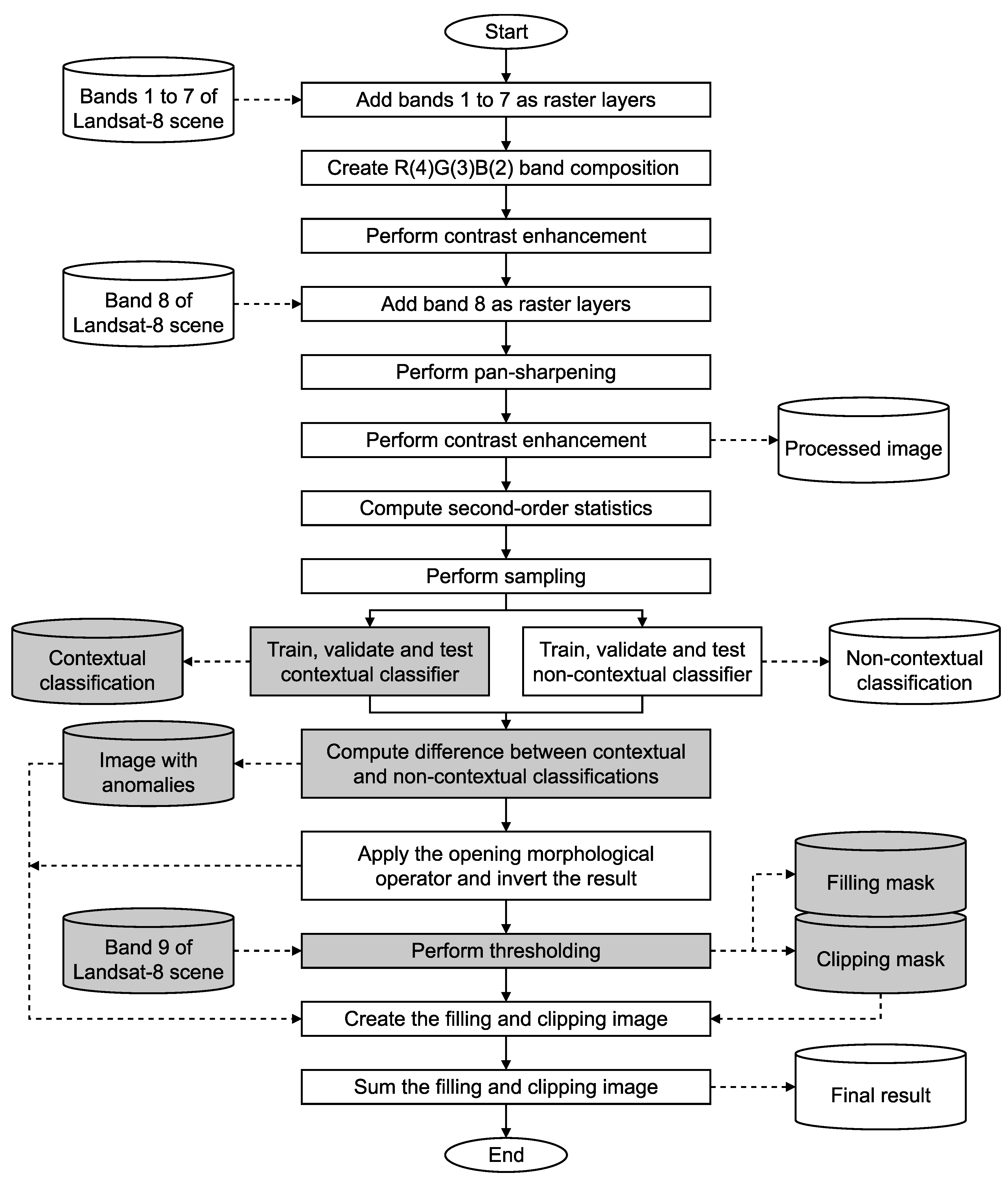
To overcome the limitations of mapping polluted water bodies in satellite images with low overlay contamination by cloud cover, we proposed a method that was based on the use of an additional image (with very low overlay contamination by cloud cover) from the same area but with a different timestamp. Figure 2 depicts a workflow that summarizes all of the major steps of the proposed methodology. More information about the parameter values of the steps can be found in the Appendix A.

The nine first steps were applied to the two images with different timestamps, as shown in Figure 2. We added the seven bands (1 to 7) as raster layers, which allowed us to create a band composition (R(4), G(3), B(2)), and then we performed contrast enhancement and added band 8 as a raster layer as well. Next, pan-sharpening and contrast enhancement were applied, resulting in the processed image. Afterwards, we computed the second-order statistics and conducted the sampling procedure. Then, using the processed image, the collected samples, and the statistical information, we performed training, validation, and classification via the non-contextual classifier.

However, the training, validation, and classification using the contextual classifier, and consequently the calculation of the difference between the contextual and non-contextual classifications results, were only performed in the image with more clouds. This was carried out because this image showed the immediate consequences of the disaster and thus allowed us to highlight the difference between the two classifications, which was not the case in the image with fewer clouds.

The image editing approaches started with the application of a morphological operator and the inversion of this result. This was followed by binarizing band 9 of the cloud-affected composite image and creating the fill-and-clip images. Finally, the sum of these two images generated the final result of the methodology. We detail the main steps required for the application of our methodology in the following sections, from image processing (i.e., a set of improvements or techniques applied to the image in order to provide more comprehensive information for some subsequent analysis, e.g., sampling or the training of the machine learning algorithms) to image editing.

3.5. Data Processing

As shown in Figure 2, firstly, the bands 1 to 7 were loaded into QGIS as raster layers for each image. A raster layer is a collection of images of the Earth’s surface that track a satellite’s movement as it rotates. The electromagnetic spectrum [1,2] bands were then superimposed to form a band combination, i.e., a single tracking image, similar to a stack structure of the seven bands.

Next, a band composition was constructed by superimposing three bands, resulting in a multi-spectral image (MS). In QGIS, this step consisted of defining the three bands that would be used for rendering the raster (which was built on the 7 bands), and it was necessary to define some other parameters, such as the metric(s) that would be used for this step. To make it easier to see the elements in the image, the composition was created using the bands R(4)G(3)B(2) to display the virtual raster in natural colors. The band composition, a vector composed of three overlapping bands, can be defined as shown in Equation (1), where $cb(x,y)$ is the composition of bands created, $b4(x,y)$ is band 4 (red), $b3(x,y)$ is band 3 (green), and $b2(x,y)$ is band 2 (blue).

$$cb(x,y)=\left[b4\right(x,y),b3(x,y),b2(x,y\left)\right]$$

(1)

Then, the mean and standard deviation were used in the band rendering—this step improved the image by increasing the contrast. Equation (2) shows that, for each band i of the N bands in the composition $g(x,y)$, the average of the pixels’ values at the position $(x,y)$ was computed, resulting in the image $m(x,y)$.

$$m(x,y)=\frac{1}{N}\sum _{i=1}^N{g}_i(x,y)$$

(2)

The standard deviation measures how far a value deviates from the mean, or the degree of dispersion. Thus, the standard deviation of the pixel’s value at position $(x,y)$ considering each of the N bands in the composition yielded the pixel’s value at position $(x,y)$ of the result $dp(x,y)$, as defined by Equation (3). Starting from a pre-defined standard deviation value, this method of histogram adjustment based on the standard deviation stretched the pixels’ values according to the average of the bands’ pixel values.

$$dp(x,p)=\sqrt{\frac{1}{N}\sum _{i=1}^N{(g_i(x,y)-m(x,y))}^2}$$

(3)

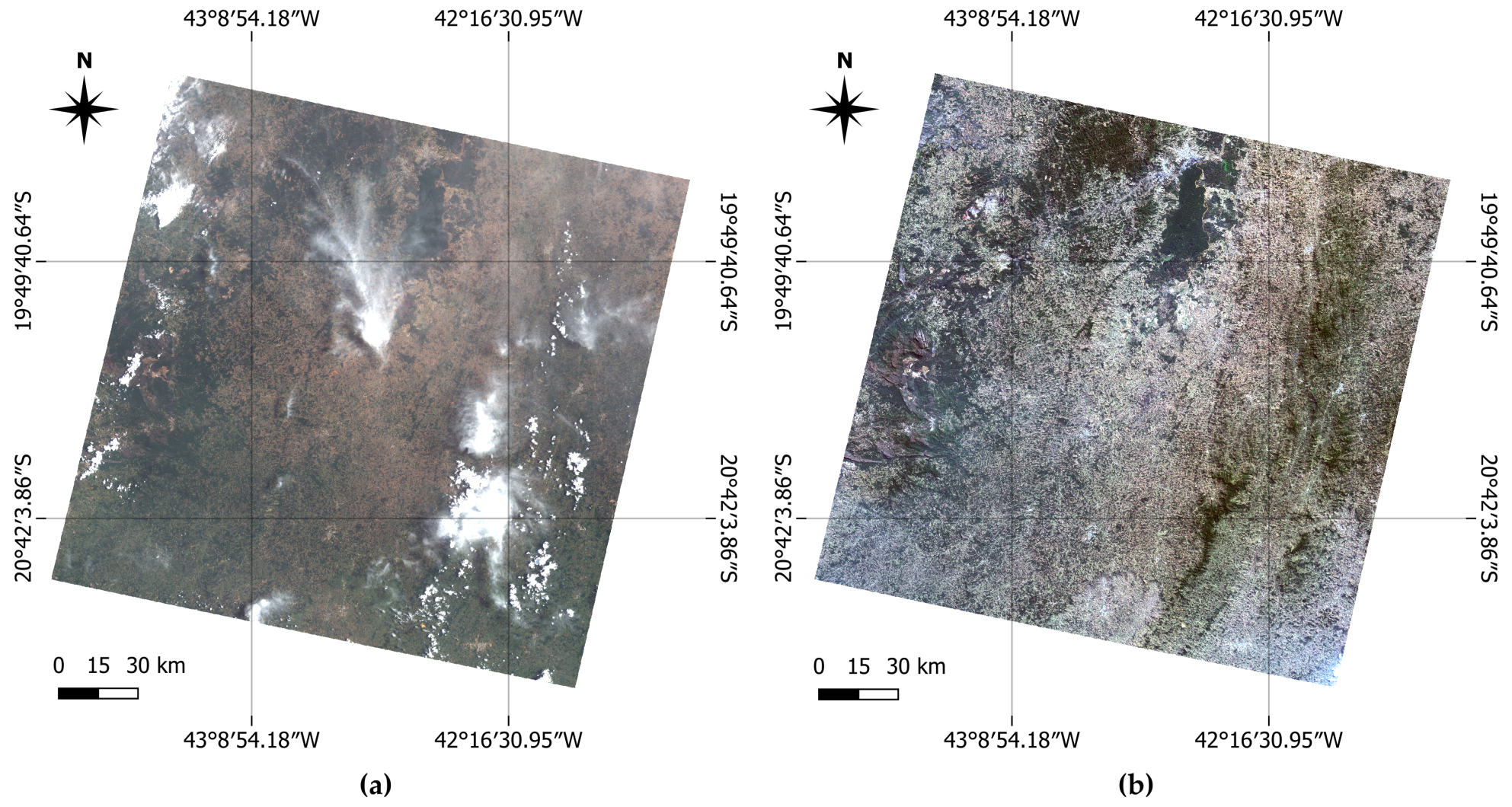
The contrast modification or stretching operation consisted of obtaining a histogram with a good distribution of occurrences along the available brightness range, improving the image contrast by changing only the mapping of the values and not the intensity of the occurrences. Figure 3 shows the results obtained after this step of the methodology, i.e., the multispectral images with low and very low overlay contamination by cloud cover with R(4)G(3)B(2) band composition and contrast enhancement.

Afterwards, the image’s band 8 (panchromatic) was then loaded as a raster layer for pan-sharpening. This method involved combining a panchromatic band (PAN, in this case the raster layer of band 8) and a multispectral image (MS, the virtual raster of band composition) to produce a high-resolution color image [53]. Then, the pan-sharpening process based on the component substitution (CS) method was used in this study. This method is expressed in Equation (4).

$$\begin{array}{cc}\hfill P{s}_k=M_k+g_k(Pc-I_L)& \\ \hfill \mathrm{where}k=1,2,\dots ,N\mathrm{and}g=[g_1,\dots ,g_k,\dots ,N]\end{array}$$

(4)

According to Equation (4), for each spectral band k, the resulting image from this step $P{s}_k$ was obtained by adding the interpolated multispectral image in the scale of the panchromatic image ($M_k$) to the result of a multiplication. The multiplication was carried out using a value $g_k$ (obtained from a gain vector g for the respective spectral band k) and the result of a subtraction. The subtraction took place between the processed panchromatic image $Pc$ and the intensity component $I_L$ (obtained by Equation (5)).

$$\begin{array}{c}\hfill I_L=\sum _{i=1}^N{w}_i{M}_i,\mathrm{where}w=[w_1,\dots ,w_i,\dots ,w_N]\end{array}$$

(5)

The multispectral image was projected onto a target space in this step, which separated the spatial structure of the spectral information into various components. The step then continued by replacing the component of the spatial structure with the panchromatic image in order to improve the transformed multispectral image. Finally, the data were returned to their original space via inverse transformation. After this step, a higher-spatial-resolution (15 m) image was produced, which helped in the analysis of the data. To perform pan-sharpening in QGIS, we first performed the superimposing sensor step, then projection (using interpolation through nearest neighbors) to prepare the virtual raster, and finally merging using the pan-sharpening (RCS—ratio component substitution) function. The obtained result was then enhanced via contrast enhancement based on the mean and standard deviation. The processed image was obtained at this point.

Later, the second-order statistics of the processed image were calculated to better understand the spatial distribution of pixels. This yielded a file containing the mean and standard deviation of the seven bands that comprised it. This type of statistical representation was used in the learning and classification steps.

The slope of the power spectrum of second-order statistics is usually close to negative two [54]. Let S be the power spectrum of an image of dimensions $M\times M$; its value can be obtained by dividing the square of the modulus of the image’s Fourier transformation result ($F(u,v)$) by the image dimensions ($M^2$). This is shown in Equation (6), where u and v are two-dimensional frequencies represented in polar coordinates, averaged in all directions $\varphi$ and for all images of the set, and f is the spatial frequency.

$$\begin{array}{c}\hfill S(u,v)=\frac{{\left|F(u,v)\right|}^2}{M^2},\mathrm{where}u=fcos\varphi \mathrm{and}v=fsin\varphi \end{array}$$

(6)

Then, the image was sampled in order to select samples to serve as training data for the classifiers. Manual selection was performed, ensuring that the samples were distributed evenly across the image. This step adopted topographic maps as the ground truth of the study area in order to validate the selected samples. To avoid biased results, samples were not drawn from the study’s main focus areas, which were ore tailing dumps (such as reservoirs or contaminated rivers). Thus, 250 samples (125 from water and 125 from non-water) were manually selected from the Doce River image with low overlay contamination by cloud cover (from 2015).

For the image with very low overlay contamination by cloud cover (from 2016), exceptionally, the sampling step required for the creation of the classifier model was performed by adapting a domain from an image of the same region but with a date prior to the disaster (2013) in order to reuse experiments that had already been carried out [16]. In summary, domain adaptation (DA) is a transfer learning approach that aims at adapting models created to solve a task in one domain to be used for a new task in another similar domain [16,55]. In this sense, based on the model created for another image (obtained from another sampling, but for the same region with a different date) and on the recalculated second-order statistics, the sampling and training steps for the image with very low overlay contamination by cloud cover (from 2016) were unnecessary.

This adaptation was similar to the sampling step, since, instead of performing this step for this domain (the image with very low overlay contamination by cloud cover from 2016), it was carried out for another (from a previous date, 2013), and this model was adapted so that it could be used by that image (from 2016) without the need to reproduce this step again, guaranteeing a result close to what would be obtained by sampling directly from the 2016 image.

3.6. Training, Validation, and Testing

After the selection of the samples, the classifiers were trained, validated, and tested. The training was carried out using the second-order statistics file, the previously selected samples, and the processed image. This step is required when creating models for classification. The classifier Boost was used for contextual classification (only on the image with low overlay contamination by cloud cover). The classifier based on decision trees was chosen for the non-contextual classification of both images, i.e., with low and very low overlay contamination by cloud cover. The main reason for this difference was the date of acquisition of the images (according to the date of the disaster), i.e., we aimed to perform non-contextual classification in both images and contextual classification only in the 2015 image (closer to the disaster, showing the differences between the two classifications).

Because the image with very low overlay contamination by cloud cover (from 2016) was taken on a later date after the disaster, the concentration of ore tailings was significantly lower on that date than in the other image. As a result, both the contextual and non-contextual classifiers produced similar results in that they detected the contaminated river and identified it as belonging to the water class. Therefore, when the difference between the two classifications was calculated, the result was close to zero. In this sense, only the non-contextual classification was used as a filler image for this image. This decision should have taken into account the classifier that produced the best results in river detection; however, due to the similarities between the two classifications obtained in this study, the non-contextual classifier was chosen at random.

The decision tree classifier constructs tree structures that assign classes to objects by verifying the decision rules present in their structure. Among the various algorithms available in the literature, Iterative Dichotomizer 3 (ID3) can be used to generate a decision tree from a dataset. Two main metrics were used for this: entropy and information gain, represented by Equations (7) and (8), respectively.

$$E\left(D\right)=-\sum _{d=1}^k{p}_k{log}_2\left(p_k\right)$$

(7)

$$G(D,a)=E\left(D\right)-\sum _{v=1}^V\frac{|D_v|}{\left|D\right|}E\left(D_v\right)$$

(8)

Thus, the entropy $E\left(D\right)$ represents the impurity of the sample set in D, i.e., the amount of uncertainty, and the gain $G(D,a)$ is the expected reduction in entropy of D when the attribute a is chosen. Such values were calculated based on a training set $D=(x_1,y_1),(x_2,y_2),\dots ,(x_m,y_m)$ with D samples, in the ratio $p_k$ ($k=1,2,\dots ,\left|D\right|$) of each type for each current sample in the set of attributes $A=a_1,a_2,\dots ,a_d$ of D (color, shape, texture, size, etc.), where $d=1,2,\dots ,k$. Also, for each attribute $a_i$, V represents a set of characteristics composed of v different values, whose representation is given by $V=a_i^1,a_i^2,\dots ,a_i^v$. Finally, $D_v$ is the subset of samples related to the value $a_i^v$ of $a_i$ in D, and $|D_v|$ represents the number of current samples in the subset.

The Boost classifier iteratively applies weak classifiers considering a distribution of weights in the training samples, so that more weight is assigned to incorrectly classified samples in other iterations. This weighted combination of weak classifiers makes Boost a strong classifier. Once the training sets were established, the weights were initialized according to Equation (9), in which $D_t(x_i,y_i)$ is the t-th distribution over all training samples.

$$\begin{array}{c}\hfill D_0(x_i,y_i)=\frac{1}{N},\mathrm{where}i=1,2,\dots ,N\end{array}$$

(9)

Then, iterations of the steps were performed for $t=1,2,\dots T$, where T is the maximum training number. For each feature, a simple linear classifier (restricted to a single feature) was trained. The weak classifier that obtained the smallest error was chosen, and, if this error was greater than or equal to $\frac{1}{2}$, the iteration was stopped; otherwise, the weight t to be assigned to the chosen classifier was calculated. The weight of the classifier was assigned as shown by Equation (10). Such an assignment guaranteed that $D_t(x_i,y_i)$ represented a normal distribution. Finally, the result of the classifier was found according to Equation (11).

$$D_{t+1}(x_i,y_i)=\frac{D_t(x_i,y_i)e^{-{\alpha }_t{y}_t{h}_t\left(x_i\right)}}{Z_t}$$

(10)

$$H\left(x\right)=sinh\sum _{t=1}^T{a}_t{h}_t\left(x\right)$$

(11)

The classification was performed using the model that was created in the previous step (training), the processed image, and the second-order statistics. As mentioned above, in order to reuse previous experiments, the classification for the image with very low overlay contamination by cloud cover (from 2016) was based on a model previously obtained for an image of the same region (but prior to the disaster, in 2013) and its statistics. Due to domain adaptation, the second order was recalculated. This step yielded a binary image with objects of the “water” class in white and objects of the “non-water” class in black.

After the classification results (contextual and non-contextual) of the image with low overlay contamination by cloud cover (from 2015) were obtained, the difference between these two results was calculated to evaluate the congruences and incongruences between the two classifiers, as it was expected that they would produce similar probability estimates during the classification step [29,43,44,45]. The difference $d(x,y)$ was calculated using Equation (12), where x and y are the pixel coordinates, $n(x,y)$ is the image produced by non-contextual classification, and $c(x,y)$ is the image produced by contextual classification.

$$d(x,y)=n(x,y)-c(x,y)$$

(12)

Incongruence is an indicator of the presence of anomalies and occurs when predictions diverge; thus, the method used to assess this situation was the divergence itself, which is responsible for measuring the difference between two probability distributions. The result of calculating the difference between the classifications of the image with low overlay contamination by cloud cover (from 2015) was an image that highlighted the differences between these classifications.

3.7. Image Editing

Later, the image editing started. To eliminate the noise in the binary image, the morphological opening operator was applied to both the result of the non-contextual classification of the image with very low overlay contamination by cloud cover (from 2016) and the result of the difference between the classifications of the image with low overlay contamination by cloud cover (from 2015, in which anomalies were identified). Equation (13) expresses the morphological opening operator. The opening $\gamma$ of an image f by a structuring element B, denoted by ${\gamma }_B\left(f\right)$, is the erosion $\epsilon$ of an image f by B (i.e., ${\epsilon }_B\left(f\right)$), followed by the dilation $\delta$ of ${\epsilon }_B\left(f\right)$ by the transposed structuring element $B^{\prime }$ [56].

$${\gamma }_B\left(f\right)={\delta }_{B^{\prime }}\left[{\epsilon }_B\left(f\right)\right]$$

(13)

The goal of an opening in a binary image is to eliminate connected white components (noise or irrelevant objects) whose area in pixels is smaller than the structuring element. The structuring element is a set that is defined in terms of its size and shape. The structuring element that was selected for this procedure was square and had a radius of one. Its center was compared to each component of the image during the process to produce the desired outcome while taking into account the neighborhood that was defined by its properties.

Next, the result of the morphological operation was inverted to show the detected water bodies in black and the remaining pixels in white, making it easier to visualize the classification. Thus, we applied $1-pv(x,y)$ for each pixel to invert the colors so that black (0) became white (1) and vice versa, where $pv(x,y)$ is the value of the pixel at the position $(x,y)$.

Then, band 9 (cirrus) of the image with low overlay contamination by cloud cover (from 2015) was binarized in accordance with Equation (14), for which $\alpha$ was the threshold. This step was performed to create the fill mask, $mp(x,y)$, which highlighted in white (i.e., $mp(x,y)=1,\mathrm{if}{b}_9(x,y)\ge \alpha$) the region affected by clouds that had to be filled in with new information while keeping the remaining pixels in black (i.e., $mp(x,y)=0,\mathrm{if}{b}_9(x,y)<\alpha$).

Shortly afterwards, the inverse of $mp(x,y)$ yielded the clipping mask $mr(x,y)$, which highlighted the cloud-free portions of the image in white and the cloud-affected portions of the image in black. For the thresholding step, the histogram of band 9 was examined in order to choose the threshold that separated intensity values according to whether they were part of dense clouds. These dense clouds did not enable the full analysis of the data.

$$mp(x,y)=\left\{\begin{array}{cc}0,\hfill & \mathrm{if}{b}_9(x,y)<\alpha \hfill \\ 1,\hfill & \mathrm{if}{b}_9(x,y)\ge \alpha \hfill \end{array}\right.$$

(14)

Next, we filled and clipped the images by multiplying the masks by the 2016 and 2015 results, respectively, after the masks had been made. This procedure created a clipped image that ignored the cloud areas, which were highlighted in black, and a filled-in image that contained the areas that needed to be rebuilt in the cloud image. Lastly, by adding the two results obtained in the multiplication step, the final result was created. This step is expressed by Equations (15)–(17).

$$ip(x,y)=mp(x,y)\ast {\gamma }_B^{\prime }\left(n_{2016}(x,y)\right)$$

(15)

$$ir(x,y)=mr(x,y)\ast {\gamma }_B^{\prime }\left(d_{2015}(x,y)\right)$$

(16)

$$rf(x,y)=ip(x,y)+ir(x,y)$$

(17)

4. Results

Three key qualifiers were used to evaluate the results since, according to Kittler et al. [18], they are typically used to qualify anomalies. Each of the following three sentences makes a comment regarding each qualifier. Since the images of the two study areas for this study were classified with a value of 9, which represents the highest quality of satellite images, the images’ high quality was ensured (Landsat 8). The Boost classifier handled the contextual classification, and the decision tree handled the non-contextual classification. By calculating the difference between these two classification results for the cloudy image, the presence of incongruence was determined (2015).

The final resulting image was carefully cropped to create a set of smaller images because the Landsat 8 satellite images cover a vast amount of territory. As the evaluations conducted in other studies referenced in the literature were conducted using smaller images, these clippings were required. The final image was cropped in this way to create 8400 clippings that each measured 151 by 193 pixels.

The clippings were then validated using the metrics of accuracy [29] ($AC$, measures the efficiency of results), precision [30] ($PR$, measures the relevance of results), recall [29] ($RE$, measures the number of relevant positive results), and F-measure [30] ($FM$, calculates the harmonic mean between precision and recall), as presented in Equations (18)–(21), where M is the number of images.

$$AC=\frac{TP+TN}{M}$$

(18)

$$PR=\frac{TP}{TP+FP}$$

(19)

$$RE=\frac{TP}{TP+FN}$$

(20)

$$FM=2\times \frac{PR\times RE}{PR+RE}$$

(21)

For this purpose, true positives ($TP$s) were defined as images/clippings in which inconsistencies were actually detected, i.e., the incongruence was correctly detected. True negatives ($TN$s) were images/clippings in which congruence was correctly detected; false negatives ($FN$s) the images/clippings in which congruences were falsely detected, i.e., incongruence was identified as congruence; and false positives ($FP$s) images/clippings in which the inconsistencies were falsely detected, i.e., when congruence was identified as incongruence.

According to the methodology, during the last step of image editing (the sum of the images), the result of the image with low overlay contamination by cloud cover (from 2015) had its regions affected by clouds filled with the result of the image with very low overlay contamination by cloud cover (from 2016). In this regard, the strategy was examined using two validations: the first one took into account the filling image when calculating the metrics, and the second one ignored this area and only took into account the clipping image’s area. The results from each of the validations are shown in the following sections.

4.1. First Validation

When considering the filling area, 23 clippings referring to unpolluted bodies of water (which were occluded by small clouds) were classified as false positives because they appeared as incongruent in the final result. On the other hand, 16 of the clippings were classified as true positives because they belonged to the section of the Doce River that was cloud-covered and contributed to its mapping in the final analysis.

Table 3. Quantitative evaluation of incongruence detections in the final result (composed of 8400 clippings) considering the filling area.

	Incongruent Event	Congruent Event
Incongruent detection	TP = 79	FP = 27
Congruent detection	FN = 5	TN = 8289

shows the values of each one of these categorizations.

4.2. Second Validation

This second validation disregarded the filling area, i.e., considered the same area studied by Dias et al. [11]. In this scenario, the 23 clippings that negatively interfered with the result (which were taken into account in the first validation) were absent. These clippings pertained to unpolluted water bodies that appeared as inconsistencies (false positives) in the final result due to small clouds. In addition, 16 clippings pertaining to the section of the Doce River that helped in mapping it were also ignored (since they corresponded to the area covered by cloud). This region was classified as true negative, i.e., it was considered to be congruent; however, it should have been categorized as a true positive, since that portion was part of the incongruent event and, therefore, represented an incongruence. Based on these categorizations, the clippings were counted.

Table 4. Quantitative evaluation of incongruence detections in the final result (composed of 8400 clippings) disregarding the filling area.

	Incongruent Event	Congruent Event
Incongruent detection	TP = 63	FP = 4
Congruent detection	FN = 5	TN = 8328

presents these values.

According to both validations, which examined in two different ways the inconsistencies that appeared in the final result of the image editing, five clippings that represented a small portion of the Doce River were detected as congruent (i.e., classified as false negatives) after applying the noise removal filter to the final result.

Once the categorizations were performed, the metrics of accuracy, precision, recall, and F-measure were determined. For the first validation, the results indicated an accuracy of $99.62\%$, precision of $74.53\%$, recall of $94.05\%$, and F-measure of $83.16\%$. As regards the second validation, an accuracy of $99.89\%$, precision of $94.03\%$, recall of $92.65\%$, and F-measure of $93.33\%$ were found. These values are presented in

Table 5. Comparison of the results obtained in this study (considering the two types of validation) with those of other studies available in the literature [9,10,11,30,33,34,35,36,37]. Values in bold indicate the top five results for each metric.

Study	Accuracy	Precision	Recall	F-Measure
Validation 2	99.89%	94.03%	92.65%	93.33%
[11]	99.78%	73.96%	100.00%	85.04%
[33]	91.20%	98.10%	95.7%	96.88%
[30]	-	96.50%	94.8%	95.64%
Validation 1	99.62%	74.53%	94.05%	83.16%
[34]	99.20%	91.85%	53.55%	67.66%
[9]	88.68%	90.62%	79.62%	84.76%
[35]	98.49%	83.84%	83.66%	83.76%
[36]	98.00%	-	-	-
[37]	78.00%	82.00%	75.00%	78.34%
[10]	84.00%	63.00%	81.00%	70.88%

.

Also, the results of other studies [9,10,11,30,33,34,35,36,37] conducted in different domains are compared to the accuracy, precision, recall, and F-measure of this study in Table 5. This comparison took into account both types of validation. Its goal was to demonstrate that the results obtained herein were comparable to those that identified outliers. Table 5 does not attempt to demonstrate which methodology is the best for identifying pollution in the Doce River, since this was not the main objective of this study.

As can be seen, the results were in line with other studies’ findings, and at least one of the values (for validation 1 or 2) was among the top five results. However, the studies presented by Qi et al. [33] and Chen et al. [30], which had excellent precision, recall, and F-measure results, made reference to particular case studies. The former alluded to a uniform area of ice in Antarctica, and the latter alluded to the fact that the images were taken at a very low altitude (implying a high precision and recall and, consequently, F-measure). In this sense, validation 1 also produced results among the five best values when compared against the other studies, which made reference to heterogeneous study areas and high image capture altitudes. The same result had its precision impaired due to the clippings that, as previously mentioned, were negatively categorized as false positives.

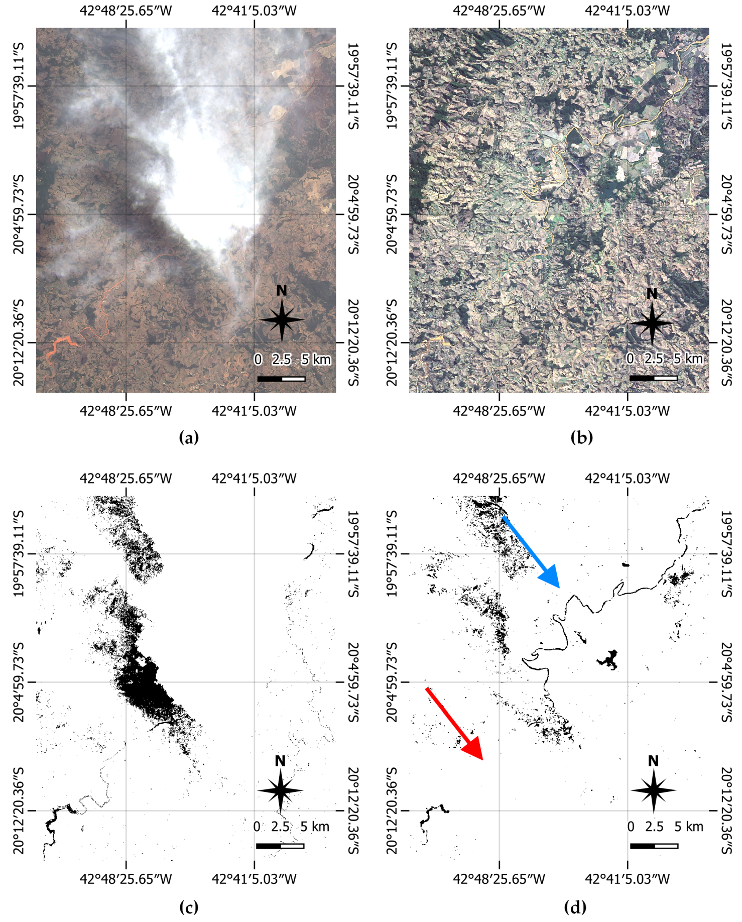
The four images in Figure 4 focus on the same study area. Figure 4a,b show images with low and very low overlay contamination by cloud cover over portions of the Doce River, from 2015 and 2016, respectively. Figure 4c shows the results of the contextual classification found in Dias’ study (it is possible to observe that the region affected by clouds was not mapped), and Figure 4d displays the application’s final result, demonstrating that the affected region had its mapping extended (indicated by the blue arrow). However, the use of the noise removal filter eliminated part of the river (indicated by the red arrow). Therefore, in order to avoid reducing the mapping of the river, the noise removal filter could have been disregarded; however, noise would be present in the final result.

5. Discussion

We used a methodology that contributes to machines learning how to extend the mapping of polluted water bodies to areas occluded by clouds, improving the detection of anomalies and overcoming the limitations imposed by the presence of clouds in images from remote sensing. These limitations were not overcome by our ADS-KT in [11]. We found that image editing allowed the analysis of the final result (in binary) without cloud interference over the Doce River (where the environmental disaster took place). Also, an analysis was conducted to understand the impact of noise removal (applied during image editing) on the output of ADS-KT. We also found that this noise removal filter did not contribute positively to the mapping of some areas. Moreover, this study was in agreement with [11], since the quantitative analysis of the proposed methodology showed that anomalies of the type unexpected structure and structural components were successfully detected by this strategy.

According to the methodology, the image editing process was carried out after the training and classification approaches, i.e., considering the results of the classifications. Due to the differences in the domains (the difference in data and the amount of ore tailings in the river), it was not possible to edit images before training and classification, i.e., directly on the processed images, since two different domains were joined so that training and classification in the same scene could be performed next.

It was noted that the contextual classifier did not take into account the water quality when deciding which class to assign for the Doce River in the image with low overlay contamination by cloud cover (from 2015) when inconsistencies were being detected. Regarding the non-contextual classifier, water could not be categorized as “water” if it was contaminated (as a result of the significant amount of debris dumped into the river). Once the outcomes differed, this situation demonstrated incongruence. Additionally, for other water bodies (such as other rivers, reservoirs, and lakes) the outputs of both classifiers were similar (with an insignificant difference in pixels), indicating congruence.

Regarding negative results, the presence of some clippings labeled as false positives was caused by the non-limitation of the study area, a fact that suggested less precision. The result of the difference between the two classifications (from the image with low overlay contamination by cloud cover) for that region of the Doce River (indicated by the red arrow in Figure 4d) was not dense enough to avoid elimination during noise removal, which led to a number of false negatives being produced. However, as shown by the quantitative results, the mapping of the cloud-affected area was successfully completed. As the studied event was related to water bodies, any other element was considered a true negative, in addition to the other rivers (aside from the Doce River) that demonstrated congruence in their classifications.

As was already mentioned, the filling mask (produced during image editing) allowed for the almost complete mapping of the Doce River (implying more clippings categorized as true positives); however, it resulted in a considerable number of false positives. Nevertheless, in contrast to other studies in the literature [9,10,11,30,33,34,35,36,37], this methodology produced noteworthy results, because at least one of the two validations placed it in the top five studies in Table 5.

6. Conclusions

This study mainly investigated whether ADS-KT in association with image editing could impact the mapping (learned by a machine) of polluted water bodies when mapping is extended to areas occluded by clouds. The focus of this study relied on detecting anomalies learned by machines, not by humans, and we expected that machines could also learn how to extend the mapping to improve the detection of anomalies, going further than the ADS-KT approach described in [11]. Additionally, an investigation of the impact of noise removal on the results reached by ADS-KT was taken into consideration.

It is concluded that this study met the objectives set forth and produced promising results. In other words, we found that the associated use of ADS-KT and the image editing technique enabled the machine to learn, with high performance, how to extend the mapping of polluted water bodies occluded by clouds.

Understanding the association of ADS-KT with image editing will help researchers applying ADS-KT in remote sensing studies to overcome the challenges faced when analyzing satellite images with overlay contamination by cloud cover. The original aspect of this study is that we edited an image resulting from the application of ADS-KT based on another image resulting from the application of ADS-KT.

A limitation of this study is that we did not find a way to remove noise without affecting the disaster mapping. For future work, a comparison of this methodology in association with other cloud removal strategies (e.g., in-painting [52], information cloning [21], the Poisson blending algorithm [20], sparse representation concepts [22,23], sparse groups [24], signal processing [25], regression trees and histogram matching [27], and deep learning [26]) is suggested.

The findings should make an important contribution to the field of remote sensing, especially for surface water monitoring. Furthermore, it is expected that this study will contribute to the world achieving UN Sustainable Development Goal 6, i.e., ensuring access to water and sanitation for all, since, according to the UN [57], access to safe water, sanitation, and hygiene is the most basic human need for health and well-being. It is also expected that our research will encourage other researchers to apply ADS-KT to other scientific areas, opening up an entirely new and wide range of applications to help the world meet other UN sustainable development goals.

References

1. Richards, J.; Jia, X. Remote Sensing Digital Image Analysis; Springer: Berlin/Heidelberg, Germany, 1999. [Google Scholar] [CrossRef]
2. Schowengerdt, R.A. Remote Sensing: Models and Methods for Image Processing, 3rd ed.; Academic Press: Burlington, NJ, USA, 2007. [Google Scholar] [CrossRef]
3. Blanzieri, E.; Melgani, F. Nearest Neighbor Classification of Remote Sensing Images with the Maximal Margin Principle. IEEE Trans. Geosci. Remote Sens. 2008, 46, 1804–1811. [Google Scholar] [CrossRef]
4. Ma, L.; Crawford, M.M.; Tian, J. Local Manifold Learning-Based k -Nearest-Neighbor for Hyperspectral Image Classification. IEEE Trans. Geosci. Remote Sens. 2010, 48, 4099–4109. [Google Scholar] [CrossRef]
5. Shen, L.; Li, C. Water body extraction from Landsat ETM+ imagery using adaboost algorithm. In Proceedings of the 2010 18th International Conference on Geoinformatics, Beijing, China, 18–20 June 2010; pp. 1–4. [Google Scholar] [CrossRef]
6. Mountrakis, G.; Im, J.; Ogole, C. Support vector machines in remote sensing: A review. ISPRS J. Photogramm. Remote Sens. 2011, 66, 247–259. [Google Scholar] [CrossRef]
7. Li, Z.; Liu, H.; Luo, C.; Li, P.; Li, H.; Xiong, Z. Industrial Wastewater Discharge Retrieval Based on Stable Nighttime Light Imagery in China from 1992 to 2010. Remote Sens. 2014, 6, 7566–7579. [Google Scholar] [CrossRef]
8. Nazeer, M.; Nichol, J.E. Combining Landsat TM/ETM+ and HJ-1 A/B CCD Sensors for Monitoring Coastal Water Quality in Hong Kong. IEEE Geosci. Remote Sens. Lett. 2015, 12, 1898–1902. [Google Scholar] [CrossRef]
9. Zhou, Z.G.; Tang, P.; Zhou, M. Detecting anomaly regions in satellite image time series based on seasonal autocorrelation analysis. ISPRS Ann. Photogramm. Remote Sens. Spat. Inf. Sci. 2016, III-3, 303–310. [Google Scholar] [CrossRef]
10. Sublime, J.; Kalinicheva, E. Automatic Post-Disaster Damage Mapping Using Deep-Learning Techniques for Change Detection: Case Study of the Tohoku Tsunami. Remote Sens. 2019, 11, 1123. [Google Scholar] [CrossRef]
11. Dias, M.A.; Silva, E.A.d.; Azevedo, S.C.d.; Casaca, W.; Statella, T.; Negri, R.G. An Incongruence-Based Anomaly Detection Strategy for Analyzing Water Pollution in Images from Remote Sensing. Remote Sens. 2020, 12, 43. [Google Scholar] [CrossRef]
12. Chang, N.B.; Vannah, B.; Jeffrey Yang, Y. Comparative Sensor Fusion Between Hyperspectral and Multispectral Satellite Sensors for Monitoring Microcystin Distribution in Lake Erie. IEEE J. Sel. Top. Appl. Earth Obs. Remote Sens. 2014, 7, 2426–2442. [Google Scholar] [CrossRef]
13. Kotchi, S.O.; Brazeau, S.; Turgeon, P.; Pelcat, Y.; Légaré, J.; Lavigne, M.P.; Essono, F.N.; Fournier, R.A.; Michel, P. Evaluation of Earth Observation Systems for Estimating Environmental Determinants of Microbial Contamination in Recreational Waters. IEEE J. Sel. Top. Appl. Earth Obs. Remote Sens. 2015, 8, 3730–3741. [Google Scholar] [CrossRef]
14. Chen, J.; Zhu, W.N.; Tian, Y.Q.; Yu, Q. Estimation of Colored Dissolved Organic Matter From Landsat-8 Imagery for Complex Inland Water: Case Study of Lake Huron. IEEE Trans. Geosci. Remote Sens. 2017, 55, 2201–2212. [Google Scholar] [CrossRef]
15. Ha, N.T.T.; Koike, K.; Nhuan, M.T.; Canh, B.D.; Thao, N.T.P.; Parsons, M. Landsat 8/OLI Two Bands Ratio Algorithm for Chlorophyll-A Concentration Mapping in Hypertrophic Waters: An Application to West Lake in Hanoi (Vietnam). IEEE J. Sel. Top. Appl. Earth Obs. Remote Sens. 2017, 10, 4919–4929. [Google Scholar] [CrossRef]
16. Dias, M.A.; Marinho, G.C.; Negri, R.G.; Casaca, W.; Muñoz, I.B.; Eler, D.M. A Machine Learning Strategy Based on Kittler’s Taxonomy to Detect Anomalies and Recognize Contexts Applied to Monitor Water Bodies in Environments. Remote Sens. 2022, 14, 2222. [Google Scholar] [CrossRef]
17. Marinho, G.C.; Júnior, W.E.M.; Dias, M.A.; Eler, D.M.; Negri, R.G.; Casaca, W. Dimensionality Reduction and Anomaly Detection Based on Kittler’s Taxonomy: Analyzing Water Bodies in Two Dimensional Spaces. Remote Sens. 2023, 15, 4085. [Google Scholar] [CrossRef]
18. Kittler, J.; Christmas, W.; De Campos, T.; Windridge, D.; Yan, F.; Illingworth, J.; Osman, M. Domain Anomaly Detection in Machine Perception: A System Architecture and Taxonomy. IEEE Trans. Pattern Anal. Mach. Intell. 2014, 36, 845–859. [Google Scholar] [CrossRef]
19. Bransford, J.D.; Brown, A.L.; Cocking, R.R. How People Learn: Brain, Mind, Experience, and School: Expanded Edition; National Academies Press: Washington, DC, USA, 1999. [Google Scholar] [CrossRef]
20. Hu, C.; Huo, L.Z.; Zhang, Z.; Tang, P. Multi-Temporal Landsat Data Automatic Cloud Removal Using Poisson Blending. IEEE Access 2020, 8, 46151–46161. [Google Scholar] [CrossRef]
21. Lin, C.H.; Tsai, P.H.; Lai, K.H.; Chen, J.Y. Cloud Removal From Multitemporal Satellite Images Using Information Cloning. IEEE Trans. Geosci. Remote Sens. 2013, 51, 232–241. [Google Scholar] [CrossRef]
22. Huang, B.; Li, Y.; Han, X.; Cui, Y.; Li, W.; Li, R. Cloud Removal From Optical Satellite Imagery With SAR Imagery Using Sparse Representation. IEEE Geosci. Remote Sens. Lett. 2015, 12, 1046–1050. [Google Scholar] [CrossRef]
23. Xu, M.; Jia, X.; Pickering, M.; Plaza, A.J. Cloud Removal Based on Sparse Representation via Multitemporal Dictionary Learning. IEEE Trans. Geosci. Remote Sens. 2016, 54, 2998–3006. [Google Scholar] [CrossRef]
24. Zhang, Y.; Wen, F.; Gao, Z.; Ling, X. A Coarse-to-Fine Framework for Cloud Removal in Remote Sensing Image Sequence. IEEE Trans. Geosci. Remote Sens. 2019, 57, 5963–5974. [Google Scholar] [CrossRef]
25. Xu, M.; Pickering, M.; Plaza, A.J.; Jia, X. Thin Cloud Removal Based on Signal Transmission Principles and Spectral Mixture Analysis. IEEE Trans. Geosci. Remote Sens. 2016, 54, 1659–1669. [Google Scholar] [CrossRef]
26. Chen, Y.; Tang, L.; Yang, X.; Fan, R.; Bilal, M.; Li, Q. Thick Clouds Removal From Multitemporal ZY-3 Satellite Images Using Deep Learning. IEEE J. Sel. Top. Appl. Earth Obs. Remote Sens. 2020, 13, 143–153. [Google Scholar] [CrossRef]
27. Helmer, E.; Ruefenacht, B. Cloud-Free Satellite Image Mosaics with Regression Trees and Histogram Matching. Photogramm. Eng. Remote Sens. 2005, 71, 1079–1089. [Google Scholar] [CrossRef]
28. Bishop, C.M. Pattern Recognition and Machine Learning (Information Science and Statistics); Springer: Berlin/Heidelberg, Germany, 2006. [Google Scholar]
29. Weinshall, D.; Zweig, A.; Hermansky, H.; Kombrink, S.; Ohl, F.W.; Anemüller, J.; Bach, J.H.; Van Gool, L.; Nater, F.; Pajdla, T.; et al. Beyond Novelty Detection: Incongruent Events, When General and Specific Classifiers Disagree. IEEE Trans. Pattern Anal. Mach. Intell. 2012, 34, 1886–1901. [Google Scholar] [CrossRef] [PubMed]
30. Chen, C.; Yang, B.; Song, S.; Peng, X.; Huang, R. Automatic Clearance Anomaly Detection for Transmission Line Corridors Utilizing UAV-Borne LIDAR Data. Remote Sens. 2018, 10, 613. [Google Scholar] [CrossRef]
31. Yu, C.; Wang, F.; Shao, Z.; Sun, T.; Wu, L.; Xu, Y. DSformer: A Double Sampling Transformer for Multivariate Time Series Long-Term Prediction. In Proceedings of the 32nd ACM International Conference on Information and Knowledge Management, Birmingham, UK, 21–25 October 2023; pp. 3062–3072. [Google Scholar] [CrossRef]
32. Bozorgtabar, B.; Mahapatra, D. Attention-Conditioned Augmentations for Self-Supervised Anomaly Detection and Localization. In Proceedings of the Thirty-Seventh AAAI Conference on Artificial Intelligence and Thirty-Fifth Conference on Innovative Applications of Artificial Intelligence and Thirteenth Symposium on Educational Advances in Artificial Intelligence, Washington, DC, USA, 7–14 February 2023; AAAI Press: Washington, DC, USA, 2023. [Google Scholar] [CrossRef]
33. Liu, Q.; Klucik, R.; Chen, C.; Grant, G.; Gallaher, D.; Lv, Q.; Shang, L. Unsupervised detection of contextual anomaly in remotely sensed data. Remote Sens. Environ. 2017, 202, 75–87. [Google Scholar] [CrossRef]
34. Bormann, K.J.; McCabe, M.F.; Evans, J.P. Satellite based observations for seasonal snow cover detection and characterisation in Australia. Remote Sens. Environ. 2012, 123, 57–71. [Google Scholar] [CrossRef]
35. Yin, S.J.; Qiao, W.; Chuanqing, W.; Xiaoling, C.; Wandong, M.; Mao, H. A robust anomaly based change detection method for time-series remote sensing images. IOP Conf. Ser. Earth Environ. Sci. 2014, 17, 012059. [Google Scholar] [CrossRef]
36. Bhaduri, K.; Das, K.; Votava, P. Distributed Anomaly Detection using Satellite Data From Multiple Modalitie. In Proceedings of the 2010 Conference on Intelligent Data Understanding (CIDU), Mountain View, CA, USA, 5–6 October 2010; pp. 109–123. [Google Scholar]
37. Chandola, V.; Vatsavai, R.R. A Gaussian Process Based Online Change Detection Algorithm for Monitoring Periodic Time Series. In Proceedings of the 2011 SIAM International Conference on Data Mining (SDM), Mesa, AZ, USA, 28–30 April 2011; pp. 95–106. [Google Scholar] [CrossRef]
38. Mayot, N.; D’Ortenzio, F.; Ribera d’Alcalà, M.; Lavigne, H.; Claustre, H. Interannual variability of the Mediterranean trophic regimes from ocean color satellites. Biogeosciences 2016, 13, 1901–1917. [Google Scholar] [CrossRef]
39. Ciancia, E.; Lacava, T.; Pergola, N.; Vellucci, V.; Antoine, D.; Satriano, V.; Tramutoli, V. Quantifying the Variability of Phytoplankton Blooms in the NW Mediterranean Sea with the Robust Satellite Techniques (RST). Remote Sens. 2021, 13, 5151. [Google Scholar] [CrossRef]
40. Documentation for QGIS 2.18. Available online: https://docs.qgis.org/2.18/en/docs/ (accessed on 11 March 2023).
41. Documentation for Orfeo ToolBox 6.4. Available online: https://www.orfeo-toolbox.org/CookBook-6.4/ (accessed on 11 March 2023).
42. United States Geological Survey. Available online: https://earthexplorer.usgs.gov/ (accessed on 11 March 2023).
43. Kittler, J.; Zor, C. A measure of surprise for incongruence detection. In Proceedings of the 2nd IET International Conference on Intelligent Signal Processing 2015 (ISP), London, UK, 1–2 December 2015; pp. 1–6. [Google Scholar] [CrossRef]
44. Ponti, M.; Kittler, J.; Riva, M.; De Campos, T.; Zor, C. A decision cognizant Kullback–Leibler divergence. Pattern Recognit. 2017, 61, 470–478. [Google Scholar] [CrossRef]
45. Kittler, J.; Zor, C. Delta Divergence: A Novel Decision Cognizant Measure of Classifier Incongruence. IEEE Trans. Cybern. 2019, 49, 2331–2343. [Google Scholar] [CrossRef] [PubMed]
46. Hodge, V.; Austin, J. A Survey of Outlier Detection Methodologies. Artif. Intell. Rev. 2004, 22, 85–126. [Google Scholar] [CrossRef]
47. Chandola, V.; Kumar, V. Outlier Detection: A Survey. ACM Comput. Surv. 2009, 41, 1–58. [Google Scholar] [CrossRef]
48. Gogoi, P.; Bhattacharyya, D.K.; Borah, B.; Kalita, J. A Survey of Outlier Detection Methods in Network Anomaly Identification. Comput. J. 2011, 54, 570–588. [Google Scholar] [CrossRef]
49. Niu, Z.; Shi, S.; Sun, J.; He, X. A Survey of Outlier Detection Methodologies and Their Applications. In Artificial Intelligence and Computational Intelligence; Deng, H., Miao, D., Lei, J., Wang, F.L., Eds.; Springer: Berlin/Heidelberg, Germany, 2011; pp. 380–387. [Google Scholar]
50. Zimek, A.; Schubert, E.; Kriegel, H.P. A survey on unsupervised outlier detection in high-dimensional numerical data. Stat. Anal. Data Min. 2012, 5, 363–387. [Google Scholar] [CrossRef]
51. Gupta, M.; Gao, J.; Aggarwal, C.C.; Han, J. Outlier Detection for Temporal Data: A Survey. IEEE Trans. Knowl. Data Eng. 2014, 26, 2250–2267. [Google Scholar] [CrossRef]
52. Maalouf, A.; Carre, P.; Augereau, B.; Fernandez-Maloigne, C. A Bandelet-Based Inpainting Technique for Clouds Removal From Remotely Sensed Images. IEEE Trans. Geosci. Remote Sens. 2009, 47, 2363–2371. [Google Scholar] [CrossRef]
53. Vivone, G.; Alparone, L.; Chanussot, J.; Dalla Mura, M.; Garzelli, A.; Licciardi, G.A.; Restaino, R.; Wald, L. A Critical Comparison Among Pansharpening Algorithms. IEEE Trans. Geosci. Remote Sens. 2015, 53, 2565–2586. [Google Scholar] [CrossRef]
54. Reinhard, E.; Shirley, P.; Ashikhmin, M.; Troscianko, T. Second Order Image Statistics in Computer Graphics. In Proceedings of the 1st Symposium on Applied Perception in Graphics and Visualization, Los Angeles, CA, USA, 7–8 August 2004; pp. 99–106. [Google Scholar] [CrossRef]
55. Tuia, D.; Persello, C.; Bruzzone, L. Domain Adaptation for the Classification of Remote Sensing Data: An Overview of Recent Advances. IEEE Geosci. Remote Sens. Mag. 2016, 4, 41–57. [Google Scholar] [CrossRef]
56. Soille, P. Morphological Image Analysis-Principles and Applications; Springer: Berlin/Heidelberg, Germany, 2003; Volume 49. [Google Scholar] [CrossRef]
57. Goal 6: Ensure Access to Water and Sanitation for All. Available online: https://www.un.org/sustainabledevelopment/water-and-sanitation/ (accessed on 20 September 2023).
Figure 1. Information about the study area: (a) its location in South America; (b) hydrographical map of the Doce River basin (Brazil); (c) overlay of an image collected by the Landsat 8 Operational Land Imager (OLI) instrument on 12 November 2015 in band composition R(4)G(3)B(2)—each band consists of the tagged image file format (TIFF).
Remotesensing 15 05760 g001
Figure 2. Flowchart of the proposed methodology to extend the mapping of the environmental disaster. In addition to the methodology presented by Dias et al. [11], the above flowchart includes steps from image editing to achieve the final results. Elements in gray represent steps that were only applied to the image with more overlay contamination by cloud cover, while elements in white represent steps that were applied to both images.
Remotesensing 15 05760 g002
Figure 3. Virtual raster with R(4)G(3)B(2) band composition and contrast-enhanced results of (a) the image with low overlay contamination by cloud cover (2015 date) and (b) the image with very low overlay contamination by cloud cover (2016 date).
Remotesensing 15 05760 g003
Figure 4. The same area of the Doce River presented in four different ways: (a) processed image from the image with low overlay contamination by cloud cover (from 2015), (b) processed image from the image with very low overlay contamination by cloud cover (from 2016), (c) the results of the contextual classification found in Dias’ study, and (d) the final result of this study. As can be seen in (d), the region affected by the cloud had its mapping completed (indicated by the blue arrow), and after applying the noise removal filter, another region was removed (indicated by the red arrow). Also, in (c), an affluent of the Doce River appears on the right-hand side of the image, meaning that it was classified as water, as well as the Doce River. Therefore, there was congruence regarding this affluent, because it was also classified as water by the non-contextual classifier. Since only incongruences appear in black in (d), this was the reason why the affluent did not appear in black in the final result.
Remotesensing 15 05760 g004