Statistical Study of the Ionospheric Slab Thickness at Beijing Midlatitude Station

Abstract

The ratio of the total electron content (TEC) to the F2-layer peak electron density (NmF2) is known as the ionospheric equivalent slab thickness (EST, also known as τ), and it is a crucial indicator of the ionosphere. Using TEC and NmF2 data from the years 2010 to 2017, this work conducts a comprehensive statistical analysis of the ionospheric slab thickness in Beijing, which is in the midlatitude of East Asia. The outcomes show that the τ have different diurnal variations at different seasons for high/low-solar-activity years. On the whole, daytime τ significantly greater than nighttime τ in summer, and it is the opposite for the τ in winter regardless of the solar cycle, whereas the τ during equinox shows different morphology for high/low-solar-activity years. Specifically, daytime τ is larger than nighttime τ during equinox in years of high-solar activity, while the opposite situation applies for the τ during equinox in years of low-solar activity. Moreover, the pre-sunrise and post-sunset peaks are most pronounced during winter for low-solar-activity years. In summer, there is a great increase in τ during the morning hours when compared with other seasons. Furthermore, the τ decreases with the solar activity during nighttime, whereas it seems there is no correlation between daytime τ and solar activity. This paper explained the primary diurnal variations in τ across different seasons during high-/low-solar-activity years by analyzing relative fluctuations of TEC and NmF2 throughout the corresponding period. In addition, based on the disturbance index (DI), which is calculated by instantaneous τ and its corresponding median, this paper found that the storm-time τ might increase when compared with its median value during the daytime, while it may both increase and decrease during the nighttime, especially around dawn and dusk hours. To further analyze the physical mechanism, an example on 2 October 2013 is also presented. The results indicate that the positive disturbance of τ during the main phase of a geomagnetic storm might be caused by the prompt penetration electric field and neutral wind during the storm, and the τ increases during the early recovery phase might be due to the disturbance dynamo electric field as well as the neutral wind during the storm. Moreover, there is a negative disturbance of τ in the recovery phase during the most disturbed sunrise hours, and it might be due to the electric field reversal, neutral wind or other factors during this period. This paper notes the differences of τ in midlatitude between different longitudinal sectors from the related climatology and storm-time behavior, as it would be helpful to improve the current understanding of τ at midlatitudes in East Asia.

1. Introduction

The ionospheric slab thickness, which is defined as the ratio of TEC to NmF2, is a crucial parameter for the ionosphere as it links the ionospheric TEC and NmF2, and it thus represents the equivalent depth of the ionosphere with a uniform electron density of NmF2. Its capacity to provide information on both TEC and NmF2 makes it a valuable tool for researching the vertical plasma distribution in the ionosphere-plasmasphere system, as well as the vertical electron density profile [1,2,3,4]. In a scientific sense, it also relates to important physical variables and ionosphere properties, such as neutral temperature and plasma scale height [3,4,5,6,7,8,9]. In terms of engineering applications, it can play a key role in fields such as ionospheric modeling and data-assimilation methodologies due to its ability to convert the TEC and NmF2 to each other [6,9,10,11,12,13]. Therefore, the field has been enriched by numerous statistical and modeling studies in the past decades since TEC measurements became available [14,15,16,17,18,19,20,21,22,23,24].

Previous research has shown that the morphology of τ varies in different regions due to its unique dependence on the solar cycle, season, local times, and geomagnetic activity at each location [25,26,27,28,29,30,31,32,33,34,35]. In addition, the impact of magnetic activity on τ remains an unresolved issue due to its susceptibility to various spatial–temporal factors, such as local time, solar activity, and location. By defining the disturbance index (DI) of τ, we found that the τ usually tends to increase during storm-time at Guam equatorial station and Yakutsk high latitude station in East Asia [34,35]. However, the morphology of the DI index in midlatitudes of East Asia has not been studied.

The τ at midlatitudes has been extensively studied as there are many TEC and NmF2 measurements in midlatitudes when compared with equatorial and high latitudes. Pignalberi et al. [6] summarized the following main conclusions derived from the existing literature: (a) There are pre-sunrise peaks irrespective of the high-and low-solar-activity years. (b) Post-sunset peaks tend to occur during the summer of medium-/high-solar-activity years, while they tend to occur during the winter of low-solar-activity years. (c) The daytime values are smaller than the nighttime ones in the winter and equinox for low-solar activity, and the reverse situation applies for summer. However, the τ in some areas does not exactly match these conclusions. For example, Jin et al. [14] found that the τ in the daytime is larger than that in the nighttime in equinoxes based on the Southern Korean GPS network. Recently, Pignalberi et al. [15] conducted a comprehensive research about the climatology of τ at midlatitudes using Wallops Island (37.9°N, 75.5°W), Roquetes (40.8°N, 0.5°E) and Chilton (51.5°N, 0.6°W) datasets, and they found some new insights into τ: (a) Winter exhibits the most pronounced pre-sunrise peak. (b) The daytime values of τ are markedly smaller than nighttime ones, irrespective of the solar activity apart from in summer. (c) There are high values during the post-sunset period 19–22 LT in some equinoctial and summer months for high-solar activity. (d) The τ is the most disturbed during nighttime and solar terminator hours. Noting that these conclusions are obtained from stations at the same geomagnetic latitude at Europe and American longitudes, and the situation in other longitudes such as East Asia longitude have not been comprehensively investigated. In addition to the study made by Jin et al. [14] described above, there are few studies that investigate the τ in midlatitude of East Asia. Wu et al. [36] also found that the τ during the nighttime is larger than that in daytime in winter, regardless of the solar activity at Xinxiang. Furthermore, summer has the highest daytime τ and winter has the highest nighttime τ. Zhou et al. [37] also drew the same conclusion based on the Qingdao datasets. Moreover, they found that daytime τ is larger than that nighttime τ in equinox for high-solar-activity years, whereas the opposite situation applies for the τ in equinox in low-solar-activity years. Therefore, the τ in midlatitude displays a complex morphology at different longitudinal sector such as East Asia which needs to be further studied.

Beijing is located in the midlatitude of East Asia and is equipped with both TEC and foF2 observation instruments. There is still much room for improvement in τ global modeling as described by previous studies, especially for τ at midlatitudes where they have most of the ionospheric equipment and the τ have different patterns from those at the other latitudes [6,16]. Previous studies on τ at midlatitudes have mainly focused on European and North American sectors in the Northern Hemisphere. There are currently a few studies available that investigate τ in the midlatitudes of East Asia. In addition, the existing research does not fully explain the reason for the variation in τ. To better understand its variation in the midlatitudes of East Asia and to improve global τ modeling, this paper studies the climatology of τ at the Beijing midlatitude station. Furthermore, this paper also preliminarily investigates the influence of geomagnetic activity on τ by utilizing the disturbance index DI of τ. This paper is organized as follows: Section 2 describes the data and methodology used for this study. Section 3 presents the results of the analysis. Section 4 interprets the results and discusses their implications. Finally, Section 5 summarizes the main contributions of this paper and suggests some directions for future research.

2. Data and Methods of Analysis

The original data (RINEX format), which served as the basis for deducing TEC, were obtained from the University NAVSTAR Consortium (UNAVCO) database (http://www.unavco.org, accessed on 18 April 2023). After that, the TEC values were derived using the software Gopi developed by Seemala (https://seemala.blogspot.com/, accessed on 18 April 2023). Additionally, a 30° elevation angle cutoff was employed to eliminate the potential multiple-path effects. Previous studies have provided detailed descriptions of the software and have compared it with other techniques. The results of these studies demonstrated that this software is capable of accurately computing TEC [38,39]. Noting that this software has been widely utilized to compute TEC in previous studies [40,41,42]. Furthermore, the regional kriging interpolation method was used to convert STEC to VTEC in this paper. This method could provide more precise VTEC values compared to using the average values of VTEC data calculated directly by the software.

The NmF2 values were calculated using the following relation: NmF2 = 1.24 × 10¹⁰ (foF2)². This formula is commonly used in ionospheric research to compute NmF2 from foF2 values [7,14]. The foF2 data utilized were obtained from the Global Ionospheric Radio Observation (GIRO) database (https://giro.uml.edu/didbase, accessed on 18 April 2023) [43]. This database provides a comprehensive collection of global ionospheric radio observation data that are freely accessible to the scientific community. It is worth noting that, in this paper, only the ionosonde data with a confidence score (CS value) greater than 80 were selected to calculate τ values. This is because data with a CS value less than 80 may contain significant errors, and using such data could lead to inaccurate results. Therefore, the selection of data with a CS value greater than 80 is crucial to ensure the reliability and accuracy of the calculated τ values. As the foF2, data had a resolution of 15 min, the TEC data were also computed with a resolution of 15 min. The τ values were then calculated by using following equation:

$$\tau =TEC/NMF2=TEC/\left(1.24\times {10}^{-6}{\left(foF2\right)}^2\right)$$

(1)

where the TEC values are measured in terms of the number of electrons per square meter, and the foF2 values are measured in terms of the critical frequency of the F2 layer, with foF2 given in megahertz (MHz). As previously mentioned, the τ values obtained from the previous equation are measured in meters. However, in the following section, the study used kilometers to measure τ for simplicity.

Since solar extreme ultraviolet (EUV) radiation serves as primary source for ionizing neutral gas in the ionosphere, this paper adopts the F10.7 index to represent solar activity. The F10.7 index is a measure of the solar radio flux at a wavelength of 10.7 cm and is widely used as an indicator of solar EUV radiation. The F10.7 index data in this study were obtained from the National Oceanic and Atmospheric Administration (NOAA) at ftp://ftp.swpc.noaa.gov/pub/indices/old_indices/ (accessed on 18 April 2023). 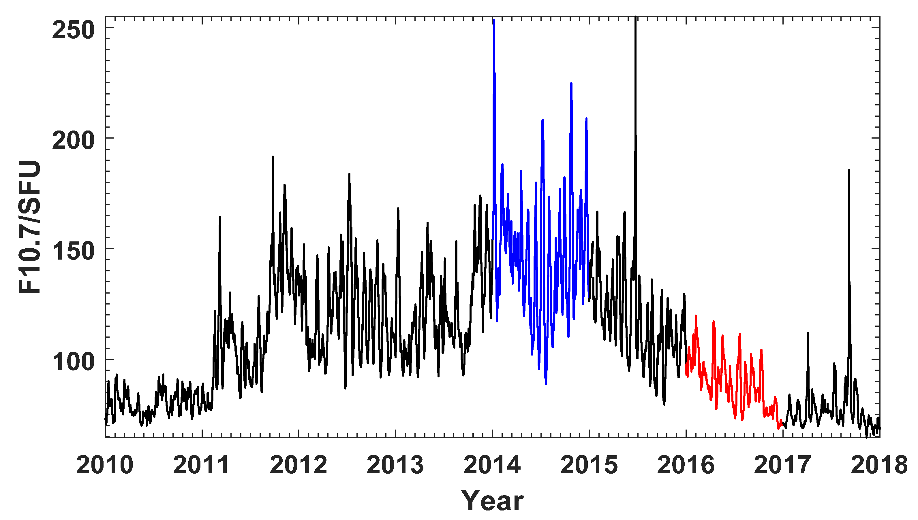Figure 1 shows the variation of the F10.7 over the period 2010–2017. The average value of F10.7 in 2014 was the highest in the 8-year period, with a value of 145.9 solar flux units (SFU). In contrast, the F10.7 index was relatively small in 2010, 2016 and 2017, with average values of 80 SFU, 88.7 SFU and 77.3 SFU, respectively. As the data availability was highest in 2016 (91.2%), this year was selected for the low-solar-activity year (blue section in Figure 1), and 2014 was selected as the high-solar-activity year (red section in Figure 1). Using Lloyd season classification, this paper split the year into three seasons: summer spanning May to August; winter spanning January to February and November to December; and equinox spanning March to April and September to October.

The impact of geomagnetic storms on τ has been a topic of research for many years. Various factors, such as the location, the solar cycle phase, and other factors, can influence how geomagnetic storms affect τ, as previous studies have demonstrated [6,25,44]. To investigate the variation of τ during geomagnetically quiet periods, data during geomagnetic storms with Dst_min < −30 were excluded, and the Dst data were downloaded from World Data Center (WDC, http://wdc.kugi.kyoto-u.ac.jp/, accessed on 18 April 2023). Pignalberi et al. [6] recently used a similar method to study the τ around the world. Noting that this paper used the median of τ rather than the mean of τ to study the climatological of τ due to this could remove the outliers of the distribution, as Pignalberi et al. [15] suggested. Moreover, in line with previous studies [34,35], we used the disturbance index (DI) to examine how geomagnetic storms affected τ and defined it as follows:

$$DI={\tau }_s/{\tau }_m$$

(2)

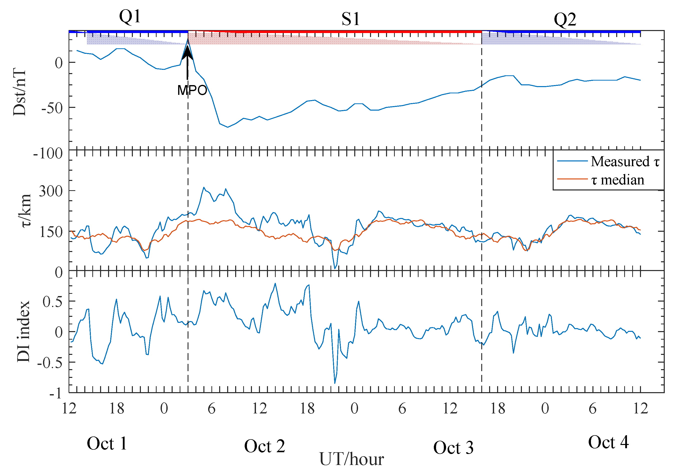
where ${\tau }_S$ and ${\tau }_m$ are the storm-time value of τ and the corresponding monthly median value of τ, respectively. Moreover, we calculated the median value of a 27-day window centered on the day of observation and used it as the monthly median value of τ. Figure 2 presents an example during the period October 1 12:00 UT–October 4 12:00 UT in 2013 in Beijing. The figure consists of three panels: the top panel shows the variation of Dst during the period, indicating that the main phase onset (MPO) of the geomagnetic storm starts at 03:00 UT on 2 October; the middle panel shows the measured τ values as a blue line and its corresponding median as a red line during the same period; the bottom panel illustrates the DI index of τ, which was calculated using Equation (2) based on the measured τ and its corresponding median value. To investigate the characteristics of the disturbance index (DI) under different geomagnetic conditions, it is important to consider both the storm-time DI index and the quiet-time DI index. As an example, Figure 2 employs the DI index during the red colored period (S1 period) to analyze the characteristics of the storm-time DI index, while the DI index with purple colored in the period (Q1, Q2 period) is utilized to study the characteristics of quiet-time DI index.

3. Results

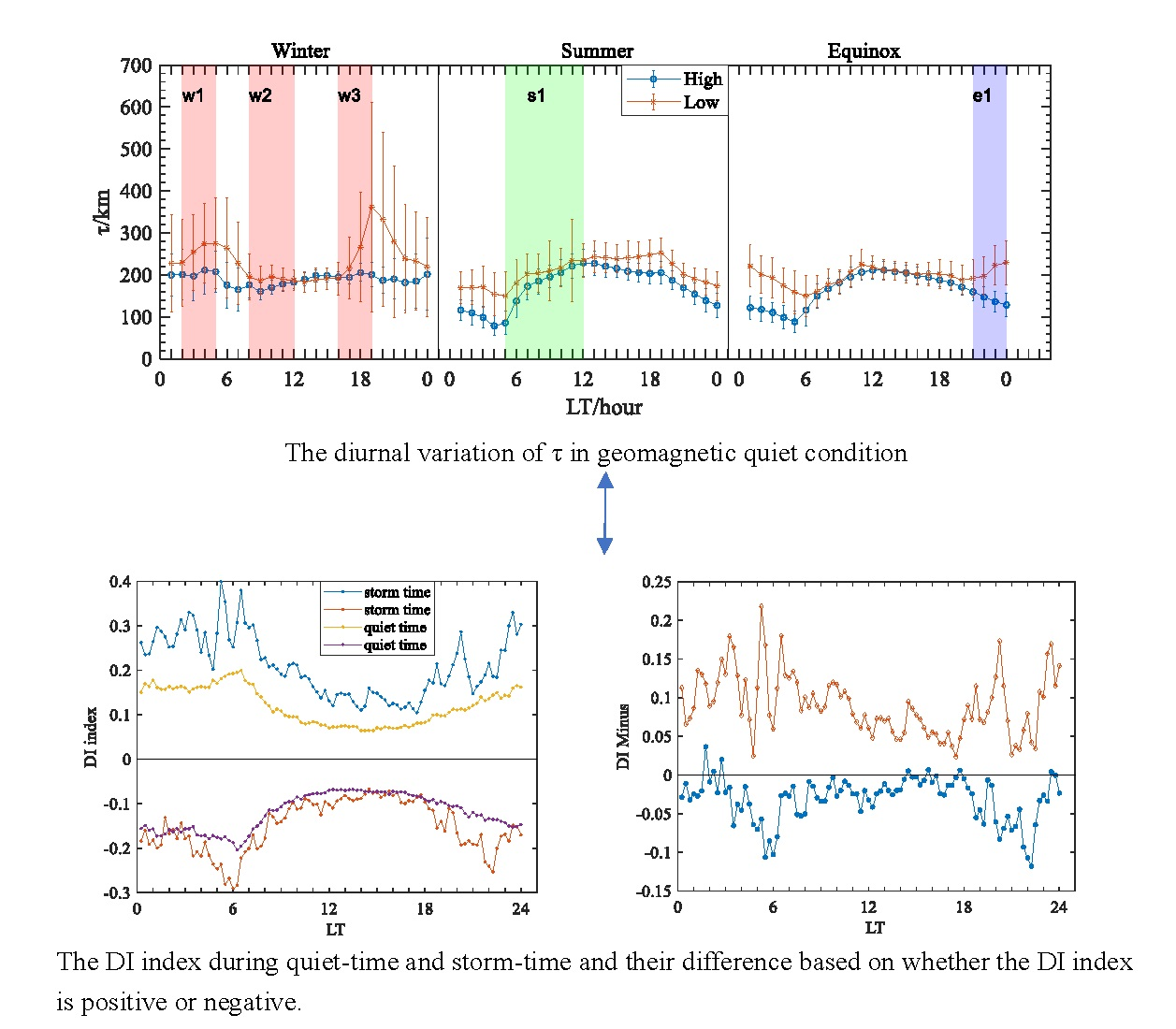
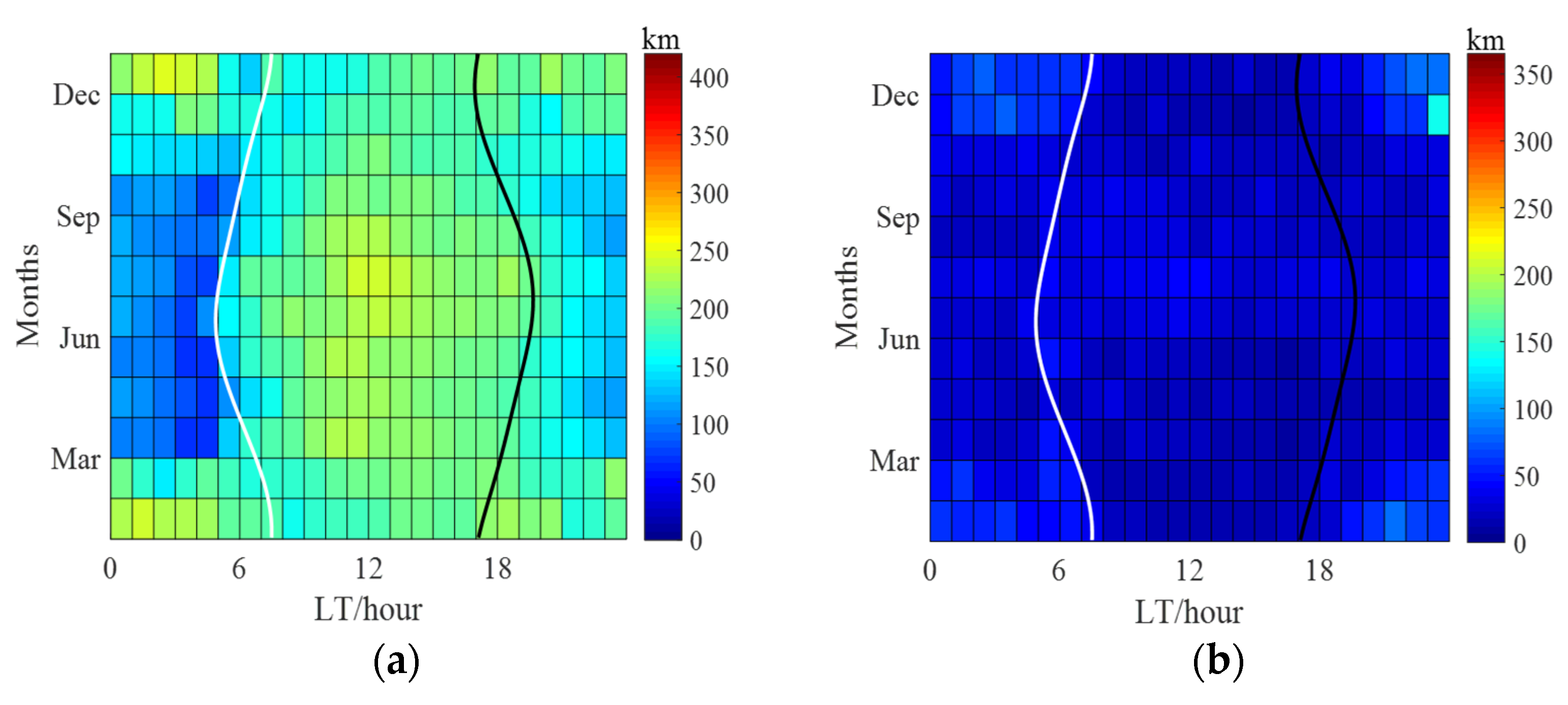
Figure 3 presents the median and standard deviation of τ on geomagnetically quiet periods based on the grid division of 0–23 LT and January–December during the 2010–2017 period in Beijing. Figure 3 also shows the time of sunrise (white lines) and sunset (black lines). As shown in the figure, the diurnal variations of τ vary considerably from season to season. Specifically, daytime τ is significantly greater than nighttime τ in summer, and it is the opposite for the τ in winter. Additionally, it can be seen that the variation of τ in equinox lies between summer and winter, and it seems that daytime τ is slightly larger than nighttime τ in equinox. In terms of the seasonal variation of τ at the same local time, daytime values are largest in summer and smallest in winter, while the opposite is true for nighttime values, which are greatest in winter and smallest in summer. In addition, there are pre-sunrise and post-sunset peaks in winter in Beijing. Furthermore, the standard deviation of τ indicates that τ varies a lot at night and during the solar terminator hours, which agrees with previous studies [6,15,34,35].

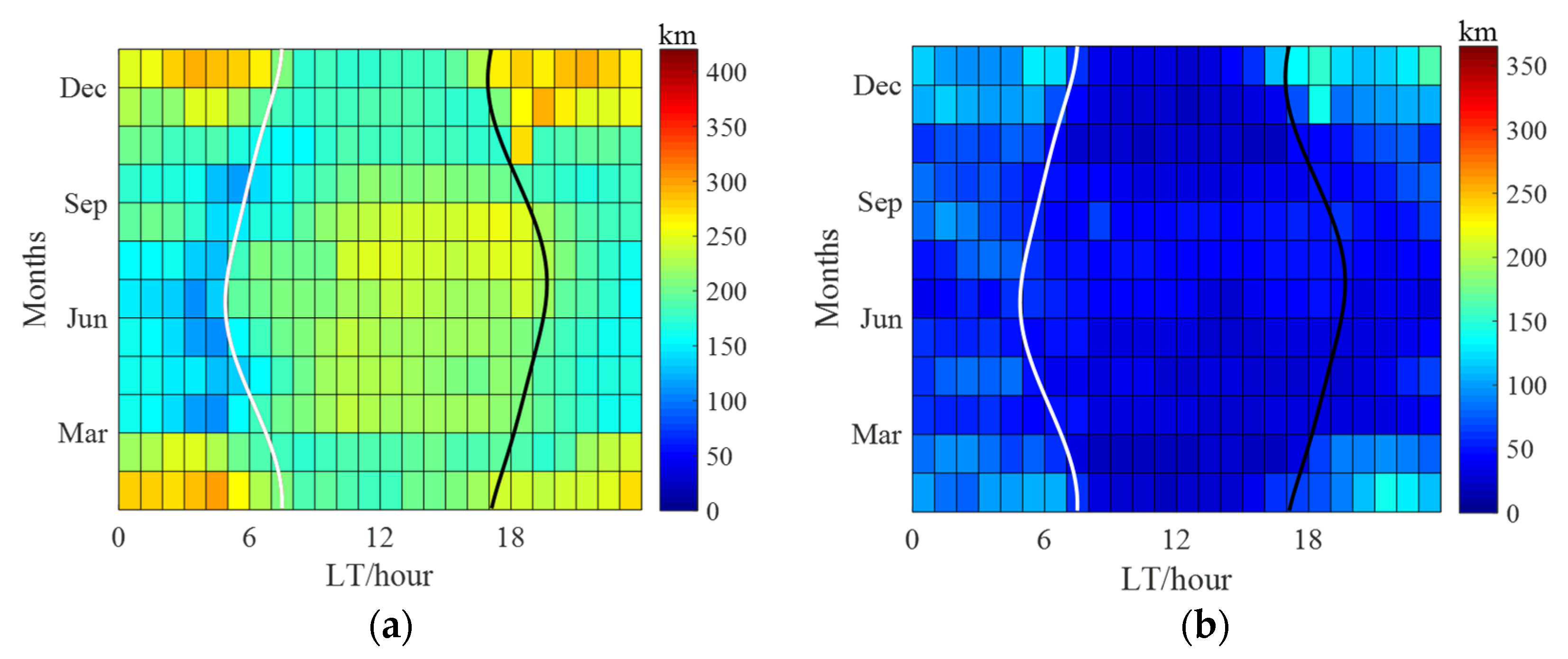
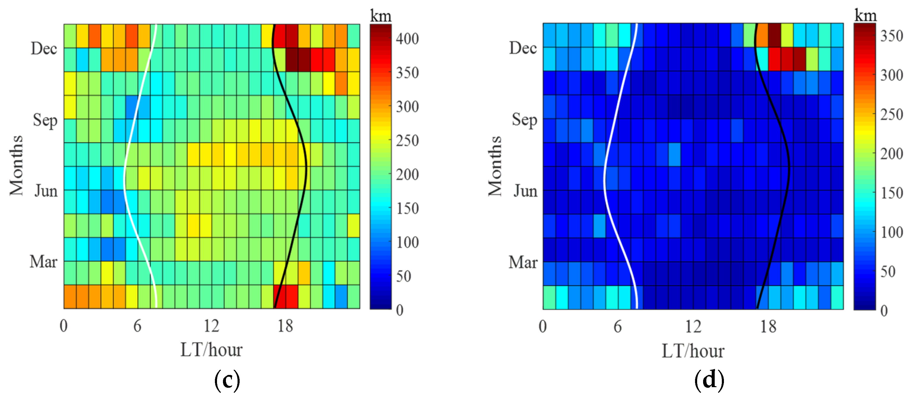
As for the solar activity dependence of τ, Figure 4 presents the median and standard deviation of τ during geomagnetic quiet-time in years of high- and low-solar-activity. Besides common features in high- and low-solar-activity years, there also exist some differences between high- and low-solar-activity years as follows:

(1)

The τ values for the high-solar-activity years are overall lower than those for all years. By contrast, the τ values for the low-solar-activity years are overall larger than those for the high-solar-activity years. It is of great importance to note that the solar activity dependence is most apparent during the nighttime, whereas it is not distinct in the daytime, consistent with the previous study conducted by Pignalberi et al. [15].

(2)

The pre-sunrise and post-sunset peaks are not apparent in winter in the high-solar-activity years, while they can be clearly seen in winter in the low-solar-activity years.

(3)

Daytime τ is larger than nighttime τ during the equinox in the high-solar-activity years, and the reverse situation applies for the τ values during the equinox in the low-solar-activity years.

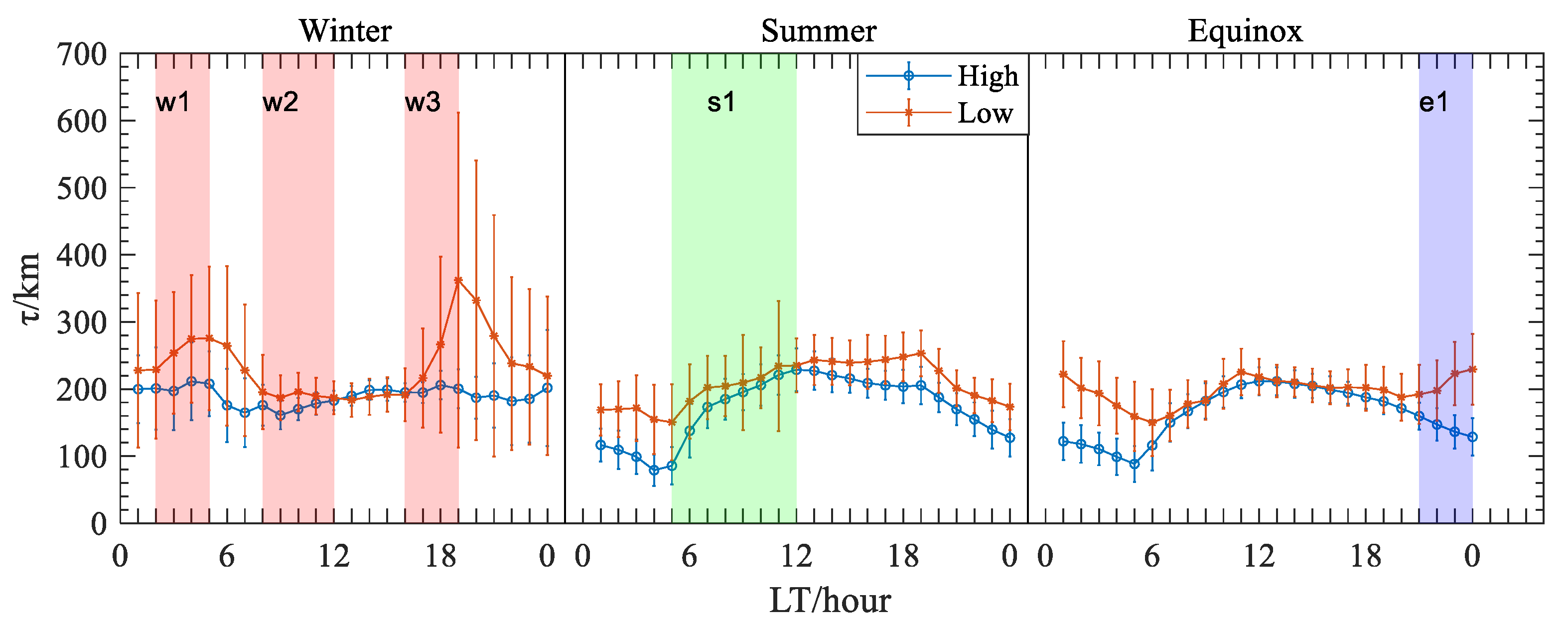
To show more clearly how τ changes throughout the day in different seasons, Figure 5 depicts the median and standard deviation of τ during the winter, summer, and equinox in the high- and low-solar-activity years. The figure highlights that the statistical characteristics of τ vary with season and solar activity:

(1)

In winter, nighttime τ are far larger than daytime τ in the low-solar-activity year, and nighttime τ are slightly greater than daytime τ in the high-solar-activity year. Moreover, the τ values in the low-solar-activity year are always greater than those in the high-solar-activity year, except for 13–15 LT, when they are slightly smaller than those in the high-solar-activity year. In addition, the pre-sunrise peak is present in both the low- and high-solar-activity years, and the peak in the low-solar-activity year is more apparent than that in the high-solar-activity year. Furthermore, the post-sunset peak is very pronounced and even surpasses the pre-sunrise peak in low-solar-activity years, while τ has only a very small peak after sunset in high-solar-activity years.

(2)

In summer, the diurnal pattern of τ in the high- and low-solar-activity years is generally consistent. In contrast to the diurnal variation in winter, daytime τ is always greater than nighttime τ in summer. Moreover, τ in the low-solar-activity years is greater than that in the high-solar-activity years during all hours, and this feature is most apparent during the nighttime. In high-/low-solar-activity years, the peak of τ does not occur before sunrise, but rather a minimal value of τ occurs before sunrise and continues to increase after sunrise with the largest increase rate during this period.

(3)

In equinox, daytime τ is greater than nighttime τ, and it has a single peak around noon hours in the high-solar-activity years. In the low-solar-activity years, the τ values have two peaks around midday and midnight hours. Moreover, the minimum value of τ appears before sunrise irrespective of the solar cycle. Additionally, τ continues to decrease after sunset in the high-solar-activity years, while τ increases after sunset until it reaches its peak around midnight in the low-solar-activity years.

(4)

The solar activity dependence is apparent for τ during the nighttime; that is, nighttime τ decreases with the solar activity irrespective of whether it is winter, summer, or equinox. However, it seems that there is no clear relationship between τ during the daytime and solar activity. The result agrees with the previous findings of Pignalberi et al. [6,15], but it also differs from the positive correlation reported by Stankov and Warnant [17] and by Davies and Liu [21].

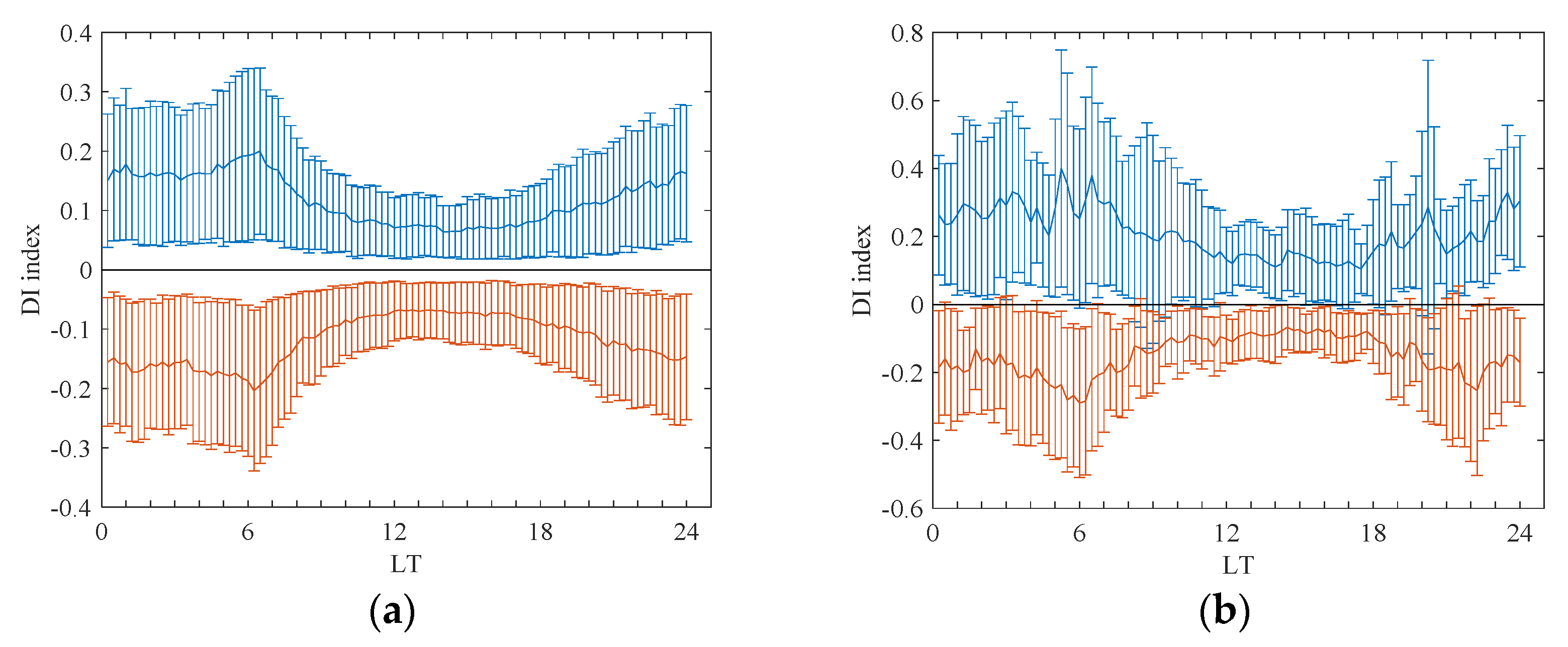
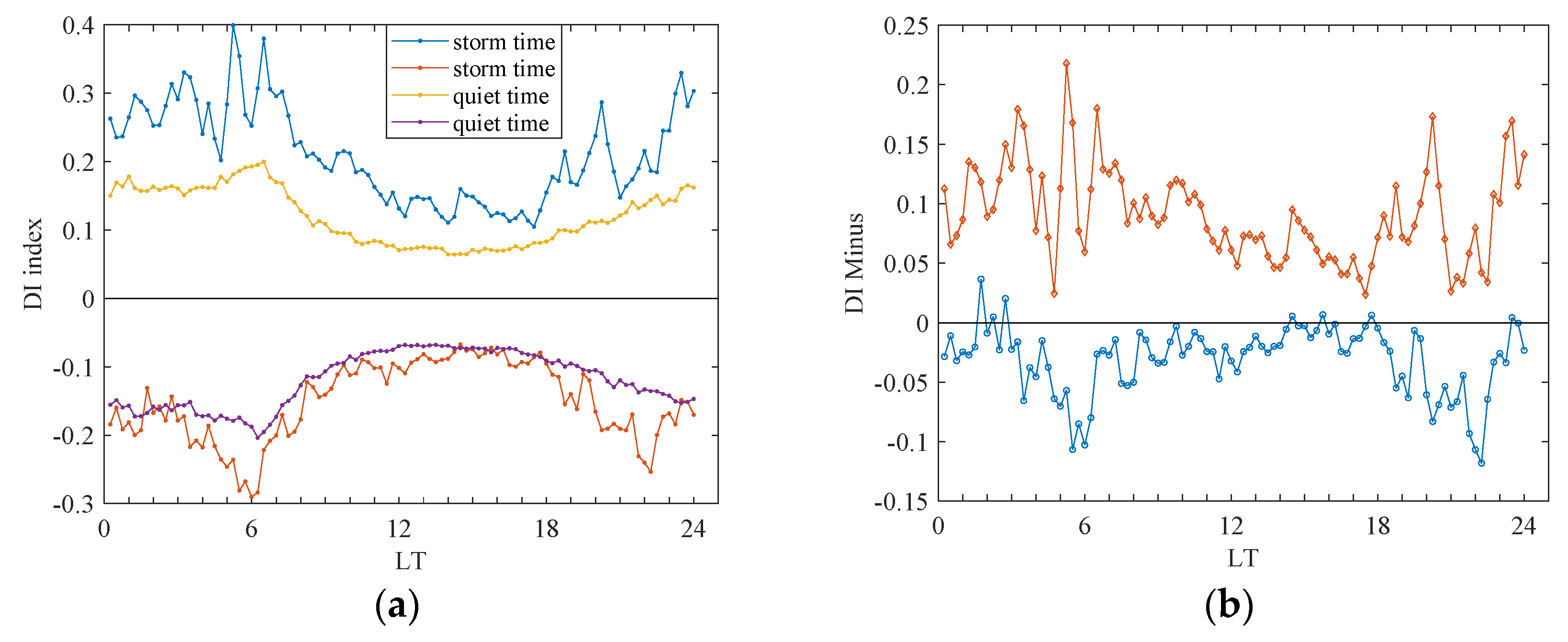
As for the geomagnetic activity dependence, the DI index described above was employed in this paper. To show how τ differs between storm-time and quiet-time, we first calculated the DI index during geomagnetic quiet-time. According to the sign of the DI, the average and standard deviation of the DI index are depicted separately. Figure 6a displays the daily variation in τ perturbation at Beijing station, with blue curves representing positive DI variations and red curves representing negative DI variations. The magnitude of the perturbation remained stable throughout the post-sunrise to sunset period, as the DI index fluctuated between −0.11 and 0.12. On the contrary, the disturbance was more pronounced during the nighttime and solar terminator hours, especially for the sunrise period, with the positive and negative DI indices being at least 0.17 and less than −0.17 between 05:00 LT and 07:00 LT, respectively. The DI index reached a maximum and a minimum of 0.2 and −0.2 at 6:30 LT and 6:15 LT, respectively.

Figure 6b illustrates the diurnal variations in the DI index for τ during storm-time. The overall variation in the DI index during storm-time is generally consistent with that during geomagnetic quiet-time but with greater fluctuations in amplitude. Specifically, the DI index varied within the range of −0.18 to 0.21 during the post-sunrise to sunset period (8:00–18:00 LT), while τ varied over a wider range, with DI indices at least greater than and less than 0.15 and −0.13 during the night and solar terminator hours, respectively. The range of the variation was the greatest around sunrise, with the maximum and minimum DI indices of 0.4 and −0.29 at 05:15 UT and 06:00 UT, respectively. Overall, the most intense disturbances in τ and the corresponding largest DI indices were observed during the night, especially during the solar terminator hours.

The effect of geomagnetic activity on τ is illustrated by comparing the DI index during quiet-time and storm-time in Figure 7a. Noting that the same DI index is displayed in Figure 6 and Figure 7a, and it enables a straightforward evaluation of how τ is affected by geomagnetic activity during stormy and quiet periods. The figure demonstrates that the range of the variation of the storm-time DI index is greater than that of the quiet-time DI index. The DI index during storm-time is higher than during quiet-time for both positive values, especially at night. The negative DI index during storm-time is slightly lower than during quiet-time in the day, but much lower than during quiet-time at night and after sunrise (6:00–8:00 LT). In order to better numerically compare the difference between the positive and negative DI indices for storm-time and quiet-time, Figure 7b shows the difference between positive and negative DI indices for storm-time and quiet-time, based on their values. It can be seen that the difference of positive DI index (larger than 0.05 for most of the period) is greater than the difference of negative DI (larger than −0.05 index) during daytime hours (07:00–18:00 LT). During the hours of sunrise and sunset, it has a relatively large value of 0.21 and 0.17, respectively. The negative DI difference fluctuates within ±0.05 for most of the period, except for the post-sunset (18:00–23:00 LT) and pre-sunrise (03:00–04:00 LT) hours, when the negative DI difference reaches the minimum values of −0.11 and −0.12, respectively. Therefore, the daytime variation in τ in Beijing during geomagnetic storms seems increased when compared with τ during geomagnetically quiet periods, while τ during the nighttime increases or decreases with a greater amplitude, especially during the solar terminator hours.

4. Discussion

Beijing is located in the midlatitudes of East Asia, and there are several factors affecting its ionospheric state. First of all, solar radiation is the most important factor influencing its ionosphere, and the summer-to-winter prevailing circulation is also one of the main contributors to the variation of the ionosphere due to it being able to cause the “winter anomaly” during the daytime at midlatitudes [44]. On the other hand, the nighttime ionosphere could be influenced by the downward plasma influx, which comes from the topside plasmasphere and conjugate hemisphere [45,46]. In addition, the reversal of the meridional wind and electric field during solar terminator hours can also have an effect on the ionosphere. In addition to the above factors that control climatology, geomagnetic activity could also cause ionospheric storms, which can have a significant influence on the ionosphere depending on the local time, solar activity, and other background states of the ionosphere–thermosphere system. These storms can be either positive or negative, and the storm-time physical drivers include the penetrating electric field, the equatorial neutral wind, the disturbance dynamo electric field, and other factors [47,48,49]. Therefore, τ at Beijing station displays a complicated pattern. As geomagnetic activity mainly contributes to ionospheric weather and results in a large ionospheric variability, this section begins by discussing the climatology of τ, and then it proceeds to analyze its variation during storm-time.

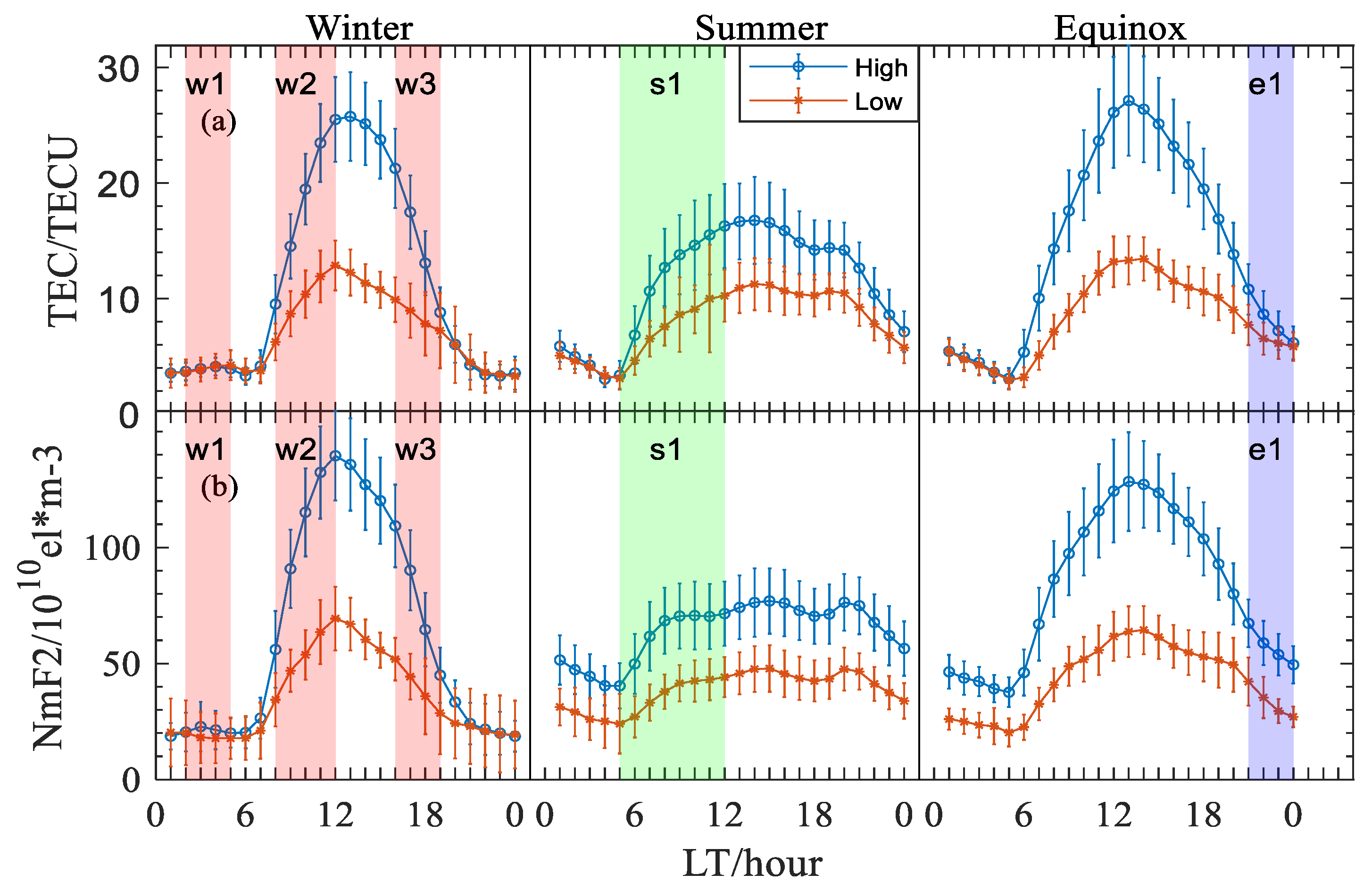
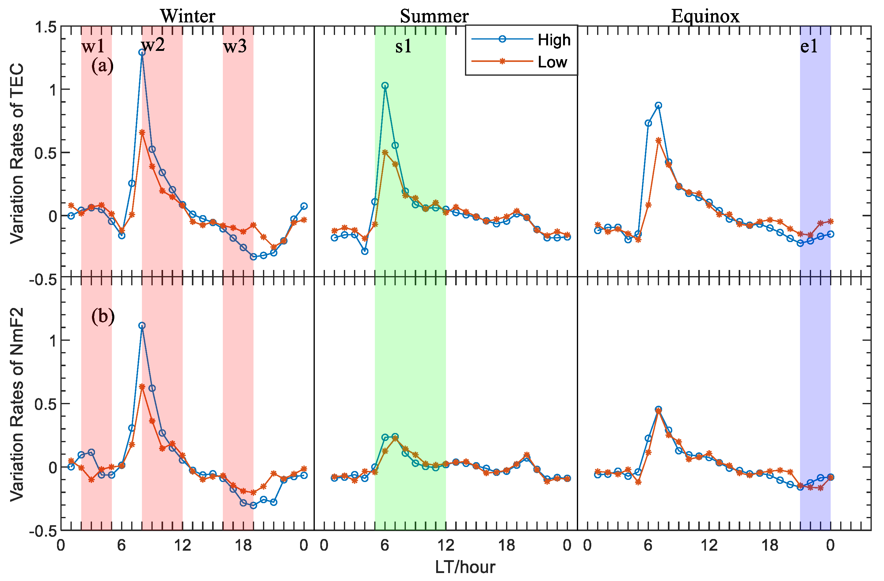
Based on the definition of τ, this paper examined TEC and NmF2 during the same geomagnetically quiet period used to examine τ in order to explain the diurnal variation in τ in different seasons in high-and low-solar-activity years, and we displayed them in Figure 8. Furthermore, the local time dependence of τ is closely related to the variation rates of TEC and NmF2, as determined using Equation (1):

$$\frac{d_{\tau }}{dt}=\frac{1}{NmF2}\frac{dTEC}{dt}-\frac{TEC}{NmF{2}^2}\frac{dNmF2}{dt}$$

(3)

Figure 9 illustrates the variation rates of τ during geomagnetically quiet periods. It can be easily determined using Equation (3) that the increase in the variation rates of τ can be classified into the following three groups: (1) the first group is when TEC increases and NmF2 decreases; (2) the second group is when TEC and NmF2 both increase, but the variation rate of TEC is greater than that of NmF2; and (3) the third group is when TEC and NmF2 both decrease, but the variation rate of NmF2 is smaller than that of TEC. The opposite situation applies for the decreases in variation rates of τ.

Figure 9 shows that the increased rates of TEC during the morning period are greater than the increased rates of NmF2 in summer and equinox, while in winter, the increase in TEC after sunrise is nearly the same as the increase in NmF2. Therefore, the value of τ in summer increases the fastest during the period from sunrise to noon, and the value of τ in summer is the maximum during this period. Comparing the curves of the TEC variation rates with the curves of the NmF2 variation rates in winter and summer in Figure 9, it can be seen that, although both parameters have high winter variation rates, the difference between the winter TEC growth rate and the summer TEC growth rate is much less than the difference between the growth rates of NmF2 in both winter (the W2 period) and summer (the S1 period). That is, the different increase rates of NmF2 and TEC between sunrise and noon in winter and summer result in the different seasonal characteristics of τ during this period. An analysis of the causes of this phenomenon in terms of the physical factors that affect ionospheric parameters in the Beijing area in both winter and summer is presented below.

Beijing station is located in the midlatitudes of East Asia, where solar radiation is the most fundamental element influencing the state of the ionosphere, followed by the summer–winter trans-equatorial circulation, which causes winter anomalies in electron density [44]. As can be seen in Figure 8, winter anomalies exist in NmF2 in both the high-/low-solar-activity years, while for TEC, winter anomalies exist in TEC in the high-solar-activity years and disappear in the low-solar-activity years. Previous studies have also found that “winter anomalies” appear in NmF2 frequently, while TEC has no “winter anomalies” in some years [50]. Therefore, the response of NmF2 to trans-equatorial summer–winter neutral winds is more sensitive than that of TEC. In terms of the factors influencing electron density at different heights, the summer-to-winter neutral wind mainly influences the electron density around hmF2. Thus, the decrease in NmF2 result from the summer–winter neutral wind (overall, NmF2 still increases due to solar altitude angle changes) leads to the increase in TEC being far greater than the increase in NmF2 during the summer morning hours, resulting in an increase in τ during the summer morning hours and the maximum daytime τ value for the year (the S1 period). However, the summer–winter neutral wind has a more pronounced winter anomaly effect on the increase in NmF2 than on the increase in TEC, which leads to a slightly greater increase in TEC than in NmF2 in winter in the high-solar-activity years and an even smaller increase in NmF2 than in TEC in the morning hours in the low-solar-activity years, resulting in a slow increase and the relatively stable state of τ in the morning hours in winter in the high- and low-solar-activity years, respectively, as shown in Figure 5.

Figure 5 shows that there is a large winter post-sunset peak of τ in the low-solar-activity years, and a less pronounced peak in winter sunset period in the high-solar-activity years (the W3 period). As shown in Figure 9, the NmF2 declines more rapidly than the TEC during the afternoon and sunset periods in both years with high-solar activity and years with low-solar activity, t which leads to a sunset peak of τ (the W3 period). The peak of τ in winter in the low-solar-activity years is probably related to the plasma descending at sunset hours, when the downward plasma influx reaches its maximum velocity [51,52,53]. When the plasma in the plasmasphere is transported from the top to the bottom and the recombination rates at higher heights are lower than those at hmF2, they are responsible for the decrease rate of TEC being less than the decrease rate of NmF2 during sunset hours. In addition, the plasmasphere at higher altitudes is exposed to more solar radiation than the F2 layer around sunset hours, as well as the meridional wind reverses to equatorward to lift up the ionosphere to a higher altitude during this period, and these phenomena are also drivers of the TEC decreasing rate being smaller than the NmF2 decreasing rate [15,16,17,35]. In summary, the field-aligned transport of plasma from the plasmasphere at sunset and the effect of more solar radiation in top ionosphere with equatorward neutral winds lead to peaks of τ in both years with high-solar-activity and years with low-solar activity. Moreover, the peaks of τ in low-solar-activity years are more pronounced because the ionospheric background O+-H+ transition heights are relatively lower in low-solar-activity years than in high-solar-activity years, resulting in a more significant effect of the transport of field-aligned plasma on the topside electron content during the nighttime, thereby increasing τ in low-solar-activity years [14,27].

Figure 5 also displays that there is a pre-sunrise peak of τ that occurs 2–3 h before sunrise (the W1 period), and there are no mechanisms for the equatorial neutral wind reversal or the exposure of the plasmasphere to solar radiation during this period. Therefore, we preliminarily infer that the pre-sunrise peaks are related to the lowering of the O+-H+ transition heights at nighttime. Moreover, the post-midnight enhancement of τ can also be seen in winter in other regions, such as South Korea and Europe, which is consistent with our results [2,14,54,55]. Furthermore, this phenomenon is the most pronounced in winter as the O+-H+ transition height is the lowest in winter, while the nighttime ionospheric O+-H+ transition height in summer is much higher than that in winter, and the effect is weak in the summer nighttime.

As for the difference in τ in equinox in the high- and low-solar-activity years, it can be seen that τ increases during the post-sunset period in the low-solar-activity years, whereas τ decreases during the same period in the high-solar-activity years (the e1 period). Figure 8 shows that TEC and NmF2 both decrease during this period; therefore, the difference may be due to the fact that TEC decreases more than NmF2 in the high-solar-activity years, while NmF2 decreases more than TEC in the low-solar-activity years, as shown in Figure 9. Moreover, Figure 9 demonstrates that the TEC variation rates in the high-solar-activity years are lower than those in the low-solar-activity years, and the opposite applies for the NmF2 variation rates, confirming this inference. The physical driver of the peaks in the low-solar-activity years may also be the strong downward plasma transport in the low-solar-activity years [15,35,54,55]. The difference between the high- and low-solar-activity years is the low background values of ionospheric electron density, TEC, NmF2 and O+-H+ transition heights in the low-solar-activity years, resulting in the downward plasma influx having an important effect on τ, and the opposite situation applies for τ in the high-solar-activity years.

It is worth highlighting that the diurnal variation in τ in equinox described above is different from the diurnal variation in τ in other midlatitude regions in the Northern Hemisphere. Based on the results of three European and American midlatitude ionospheric stations, Pignalberi et al. [15] reported that the values of τ during the daytime are smaller than those during the nighttime in winter and equinox irrespective of solar activity. Moreover, in a recent review study, they comprehensively summarized findings demonstrating that daytime τ is smaller than nighttime τ in winter and equinox during low-solar activity. However, they also found that the daytime values in the autumn equinox are larger than the nighttime values in high-solar-activity years in Hermanus, which is located in the midlatitude of South Africa [6]. Jin et al. [14] also reported that the daytime values are larger than the nighttime ones during equinox in South Korea in the moderate-solar-activity year 2003. In addition, Zhou et al. [37] found that τ in the daytime is larger than that in the nighttime in equinox in high-solar-activity years, while the reverse situation applies for τ in equinox in low-solar-activity years. This paper found larger daytime values in the high-solar-activity year 2014 and larger nighttime values, which might be due to the lowering of the O+-H+ transition height, in the low-solar-activity year 2016, results that are consistent with those of previous studies of τ in the midlatitudes of East Asia. Therefore, the τ values in equinox show different variations for different midlatitude sectors, and they still need further investigation.

Geomagnetic storms greatly influence the state of the ionosphere, as they trigger various processes that can severely disrupt the ionosphere–thermosphere system. Previous research has indicated that the relationship between τ and geomagnetic activity varies based on various spatial–temporal factors, such as location, local time, season, and other factors, such as solar and magnetic activity intensity [6,9,16,17]. At midlatitudes, there is controversy about τ during geomagnetic storms [16,19,22,31]. Bhonsle et al. [19] found that the relationship between τ and the geomagnetic index Kp appears to be ambiguous, with τ increasing and decreasing according to the season. Moreover, Fox et al. [22] found that there is no significant difference between τ in geomagnetically quiet periods and geomagnetic storms. It is worth noting that the two studies described above were conducted at midlatitude stations in North America. On the contrary, there are several studies showing that τ tends to increase during geomagnetic storms at midlatitude stations in Europe. For example, Jayachandran et al. [16] examined the impact of geomagnetic disturbances on τ by comparing the diurnal patterns of τ during magnetically quiet days with an Ap < 10 nT with those observed during disturbed days, and the results showed that τ tends to increase during both daytime and nighttime periods at the midlatitudinal Boulder station. Based on several European mid-to-high-latitude stations and using the super-posed epoch method, Gulyaeva and Stanislawska [31] found that τ tends to increase immediately after the onset of a geomagnetic storm at the solar maximum, whereas 12 to 24 h after the start of the geomagnetic storm, τ begins to increase at the solar minimum. It is of great importance to note that this conclusion is based on the τ values for 12, 24, 36, and 48 h after the storm onset. Stankov and Warnant [17] also found that τ at the European midlatitude station Dourbes increased significantly during the main phases and early stages of two severe geomagnetic storms, with Dstmin close to −400 nT. Therefore, τ seems to have different storm-time behavior in the midlatitudes of different longitudinal sectors.

As for the storm-time variation in τ in the midlatitudes of East Asia, we defined the DI index of τ in the same manner as previous studies to study the influence of geomagnetic storms on τ at Beijing station [34,35]. The results show that the differences between the positive and negative DI indices during storm and the positive and negative DI indices during quiet days are below 0.11 and above −0.05 during the daytime hours (07:00–18:00 LT), respectively. Furthermore, the differences are relatively large around dawn and dusk, reaching 0.24 and 0.19 for the positive DI index and −0.11 and −0.12 for the negative DI index, respectively. From this perspective, the results indicate that, during geomagnetic storms, the τ value in Beijing might slightly increase during the daytime, while it may both increase and decrease during the nighttime, especially around sunrise and sunset hours. Taking Figure 2 as an example, the storm-time τ values increase when compared with the monthly median values from 03:00 to 18:00 UT (11:00–02:00 LT), which is the main phase and early recovery phase of this storm, consistent with the result of Stankov and Warnant [17]. Moreover, τ decreases during the 20:00–00:00 UT (04:00–08:00 LT) period, which is the second half of the recovery phase. Therefore, the morphology of τ during this storm confirms the result in Figure 7b. In the following section, we use the example of 2–3 October 2013 to examine why τ shows such a variation during geomagnetic storms. Noteworthy is that the variation in Dst during geomagnetic storms is displayed in Figure 2.

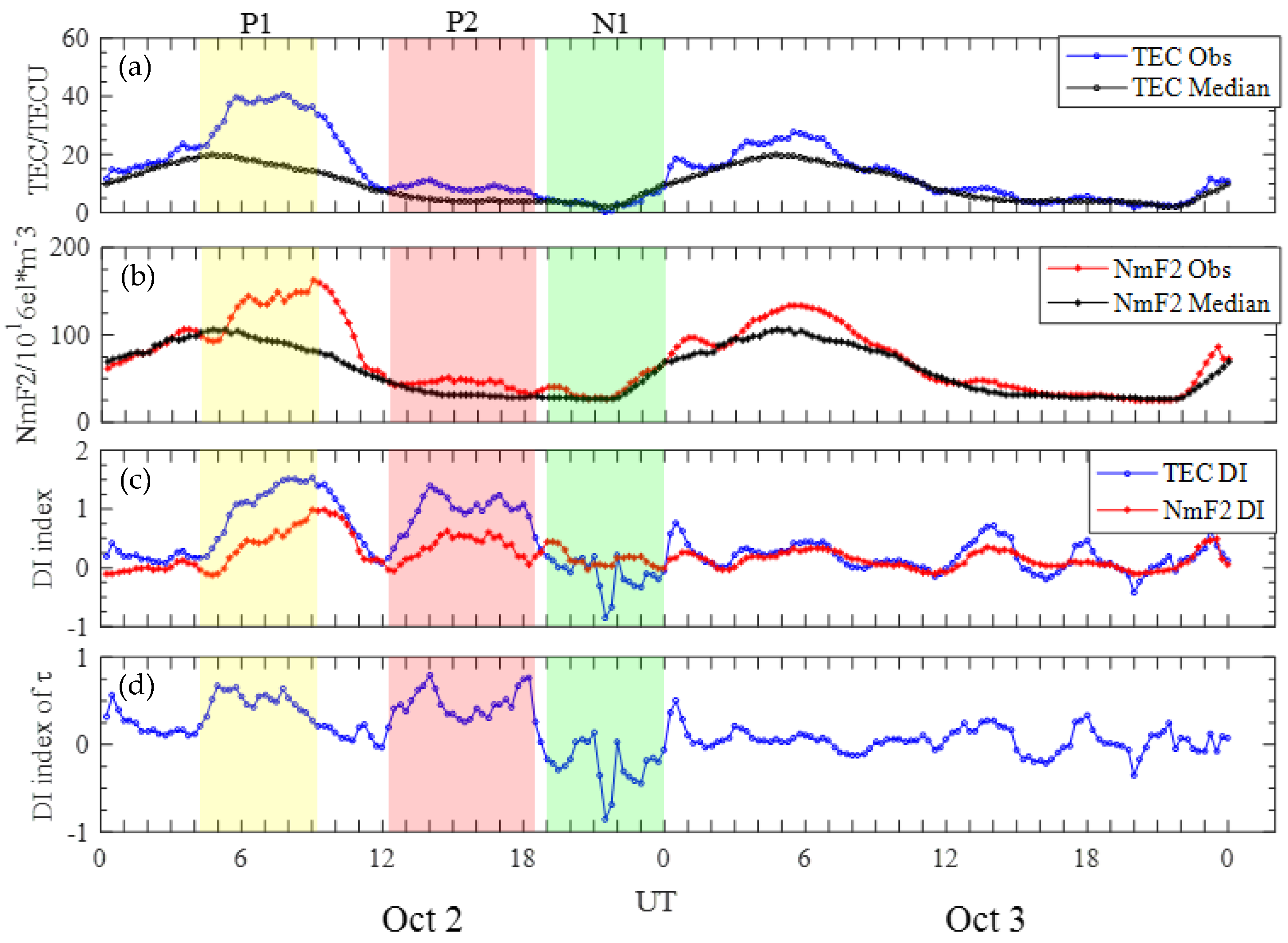
During geomagnetic storms, various processes can affect τ, including (1) the prompt penetration electric field caused by an imbalance between the R1 (region 1) and R2 (region 2) field-aligned currents (FACs), (2) equatorward neutral winds resulting from particle precipitation and Joule heating at high latitudes, (3) the disturbance dynamo electric field caused by equatorward neutral winds during the storm, and (4) composition changes transported by the storm-time equatorward neutral wind. To explain the variation in τ during storm-time, Figure 10 illustrates the changes in the DI indices in TEC, NmF2, and τ from 2 October at 0:00 UT to 4 October at 0:00 UT. Additionally, Figure 10 presents the TEC and NmF2 observations and their monthly median values.

Figure 10 shows that there is a positive disturbance of TEC from 04:15 to 08:15 UT (the P1 period), which occurs in the main phase of this storm, and there is a positive disturbance of NmF2 during this period, but not from 04:15 to 5:30 UT, when the DI index of NmF2 is negative. In this period, the positive DI index of TEC exceeds that of NmF2, leading to a positive disturbance of τ in the main phase of the storm. There is a generally a consensus that, at this latitude, the positive disturbance is primarily driven by the prompt penetration electric field and the storm-time equatorward wind [47,48]. The daytime prompt penetration electric field would lift plasma in the bottomside ionosphere to a higher altitude, where the recombination rates of electrons are lower. At the same time, the bottom ionosphere would be compensated by daytime ionization. Moreover, the equatorward neutral wind would push the ionosphere to a higher altitude during the storm. Therefore, there is a greater increase in TEC and a rather smaller increase in NmF2, resulting in τ increasing during the main phase of storm at Beijing station. Mao et al. [56] studied how the ionosphere responded to this storm in China., and the result also shows that the topside ionosphere has a stronger enhancement than the bottomside ionosphere at Beijing station, consistent with this study. Noting that there is a decrease in NmF2 from 04:15 to 05:30 UT in the P1 period, and TEC is slightly increased during this period, resulting in the positive disturbance of τ. Moreover, a decrease in NmF2 during this period could also be seen at Mohe and Xian, as shown in the work conducted by Mao et al. [56], with hmF2 being found to increase at these stations. Therefore, these findings could be attributed to the servo mechanisms proposed by Rishbeth et al. [57], and there is no prompt penetration electric field from 04:15 to 05:30 UT, as TEC does not show abrupt increases in this daytime period.

As shown in Figure 10, TEC and NmF2 both increase from 12:15 to 18:30 UT, which is the early recovery phase of the storm (the P2 period). In addition, the positive disturbance of TEC is greater than that of NmF2, leading to the positive disturbance of τ. Considering that it has entered the recovery phase, a disturbance dynamo electric field (DDEF) could exist during this period. As the DDEF is eastward during the nighttime, it would lift up the ionosphere to a higher altitude. Moreover, the storm-time neutral wind along with the nighttime equatorward neutral wind would also have an effect on the ionosphere and lift it up to a higher altitude, where the recombination rates of electrons are lower, resulting in an increase in TEC and NmF2. As the topside ionosphere has lower recombination rates, TEC could increase faster than NmF2. However, the composition disturbance zone would decrease TEC and NmF2, and it would mainly affect the ionosphere around hmF2, resulting in the decrease in NmF2 being larger than that in TEC. Therefore, the DDEF and storm-time equatorward neutral wind have a larger effect on TEC and NmF2 than the composition changes during this period, resulting in the increase in τ in the early recovery phase of the storm. It is worth noting that Lei et al. [58] found that the F2 peak and the topside ionosphere exhibit contrasting behaviors at the low latitudes of the East Asian stations Sanya and Guam, and they attributed this to the equatorward wind. In addition, they proposed that the DDEF could also play an important role in this phenomenon, confirming the inference described above.

As for the negative disturbance of τ during the P3 time interval, it can be seen that NmF2 is relatively stable during this period, and TEC decreases, especially during the time period between 21:00 and 22:00 UT (5:00 and 6:00 LT), resulting in a notable decrease in τ during this sunrise period. Previous studies have shown that the solar terminator hours are the most disturbed period for τ [6,15,34,35]. Moreover, this paper shows that the most disturbed time for τ is around sunrise and sunset times. As for the decrease in TEC, it might be due to the electric field reversal, resulting in the lowering of the ionosphere. Moreover, there is no solar radiation during this period (5:00–6:00 LT), resulting in a great decrease in topside TEC, which contains most of the TEC. In addition, the composition changes might also contribute to the TEC decreases. However, the uplifted ionosphere caused by the equatorward neutral wind has the largest effect on the F2 region in the midlatitude [44], which might be responsible for NmF2 not decreasing during this period. Therefore, the negative disturbance mainly occurred in the topside ionosphere, which caused TEC to decrease greatly, NmF2 to vary a little, and τ to decrease during this period.

Noteworthy is that the variations in TEC, NmF2, and τ during this storm are only examples. Figure 7b shows that τ could decrease significantly during the sunset period, which is not shown in Figure 10. In addition, the positive disturbance during the P1 period is larger than that shown in Figure 6b, as the disturbance shown in Figure 6 is only the mean values of the positive DI index, and there are also small positive DI indices during the daytime geomagnetic storm. As the ionospheric response to geomagnetic storms depends on geolocation, local time, solar activity, and other spatial–temporal factors, τ has other types of responses to geomagnetic storms at Beijing station. Moreover, geomagnetic storms seem to have different effects in the midlatitudes of European and American sectors. Therefore, more observations and classification work are needed in the future to explore the physical mechanism of different storm-time behaviors of τ in the midlatitudes of East Asia.

5. Conclusions

Based on the TEC and NmF2 data for the years of 2010–2017, this paper presents a statistical study of τ at Beijing station, which is located in the midlatitudes of East Asia. The results demonstrate that τ exhibits significant variations according to local time, season, solar activity, and geomagnetic activity. In addition, the climatology and storm behavior of τ are different to those in other midlatitude regions. The main conclusions of this paper can be summarized as follows:

(1)

Daytime τ is significantly greater than nighttime τ in summer, and the opposite applies for τ in winter regardless of the solar cycle, consistent with previous studies. Moreover, the largest and smallest increases in τ during the morning hours in summer and winter, respectively, are due to the prevailing summer-to-winter circulation.

(2)

Daytime τ is larger than nighttime τ in equinox in high-solar-activity years, while the opposite situation applies for τ in equinox in low-solar-activity years. This result is different from previous results in other longitudinal sectors, but it is consistent with that in previous studies in East Asia. Moreover, the post-sunset increases in τ in low-solar-activity years may be due to the lowering of the O+-H+ transition height.

(3)

The pre-sunrise and post-sunset peaks of τ are the most pronounced in winter in low-solar-activity years; this is because of the most intense downward plasma transport from the plasmasphere and the conjugate hemisphere and the resulting descent of the O+-H+ transition height in winter in low-solar-activity years.

(4)

Nighttime τ decreases with solar activity, while it seems that there is no relationship between daytime τ and solar activity, consistent with the result of Pignalberi et al. [6,15].

(5)

Storm-time τ might increase during the daytime with the effect of the prompt penetration electric field and the storm-time equatorward neutral wind, while it may both increase and decrease during the nighttime with the disturbance of the dynamo electric field, the equatorward neutral wind, composition changes, and other factors, especially around the sunrise and sunset hours when the neutral wind and electric field reverse.

These results would complement analyses of τ behavior during geomagnetically quiet and disturbed conditions in the midlatitudes of East Asia.

It is of great importance to note that there are similarities and differences between τ in the midlatitudes of different longitudinal sectors, and we will conduct more studies in this field in the future. Moreover, not only does the effect of geomagnetic activity on τ include the situations described above, but it also includes other situations, and they may depend on local time, season, solar activity, and ionospheric background when a storm occurs. Therefore, more observations and classification work will be conducted in the future to study the physical mechanism of the storm-time behavior of τ in the midlatitudes of East Asia.