Water Storage Variations Recovered from Global Navigation Satellite System Network Using Spatial Constraints: A Case Study of the Contiguous United States

Abstract

Global Navigation Satellite System (GNSS) vertical displacements are widely used to infer terrestrial water storage (TWS) variations. The traditional Laplacian inversion requires dedicated efforts to determine the optimal parameters, which has an important effect on the spatial patterns. In this study, we develop a new GNSS inversion method with flexible spatial constraints. One major merit is that the new method only requires loose boundary conditions rather than optimal parameters. A closed-loop simulation shows that the inversion using spatial constraints is improved by 7–21% compared with the Laplacian constraints. We apply this method to 18 watersheds across the Contiguous United States (CONUS) to infer daily TWS variations from January 2018 to August 2022. The results show that the amplitudes of monthly TWS time series from the spatial and Laplacian constraints are comparable to the Gravity Recovery and Climate Experiment (GRACE) Follow-On (GFO) in 16 watersheds. Furthermore, the standard deviation between the spatial constraints and GFO is at the same level as that between the Laplacian constraints and GFO. We also extract the daily TWS variations caused by heavy precipitation events in California. Our results demonstrate that spatial constraint inversion supplements the existing constraint strategies of GNSS inversion in hydrogeodesy; therefore, spatial constraint inversion can be an alternative tool for GNSS inversion.

1. Introduction

Accurately monitoring and quantifying terrestrial water storage (TWS) changes is of great importance for investigating the water available for humans and natural systems [1,2]. Satellite gravimetry, e.g., Gravity Recovery and Climate Experiment (GRACE) and GRACE Follow-On (GFO), which were launched in March 2002 and May 2018, respectively, provides a new tool used to study global mass transports, such as the terrestrial water cycle and ice sheet and glacier mass balance, at a global scale at an approximately 300–500 km spatial resolution and monthly temporal resolution [3]. Due to their coarse spatial resolution, GRACE and GFO are more sensitive to large-scale mass variations, and it is challenging to subtract high-frequency TWS changes, e.g., on a sub-monthly time scale.

The Global Navigation Satellite System (GNSS) can be used to infer regional TWS variations independently. The solid earth deforms due to the Earth’s mass changes, including water, snow, ice and atmosphere, and GNSS accurately measures this deformation with millimeter-level precision [4,5,6]. The elastic response can be theoretically modeled using loading theory [7,8]. With displacements from densely distributed GNSS stations and Green’s functions, the seasonal TWS changes have been inferred for the first time in California at a resolution of 50 km [4]. Subsequently, TWS variations are inverted at various spatiotemporal scales in the continental United States (CONUS) [1,5,6,9,10,11,12] and China [13,14,15,16,17,18,19,20]. For example, Brosa et al. inverted the mass loss during a severe drought period in the western United States, which shows consistency with the decreases in precipitation and streamflow [6]. Fu et al. recovered the seasonal TWS variations in the northwest of the CONUS; they show that the GNSS can be independently used to estimate the TWS variations. The mass changes in dry and wet periods can be inferred using the GNSS, and it can fill the gap between GRACE and GFO [1]. Zhang and Jin estimated the monthly evapotranspiration variation using the GNSS-derived TWS in the Mississippi River basin; the results indicate strong agreement between the evapotranspiration variations obtained from the GNSS and other remote sensing datasets [9]. Liu et al. recovered the TWS in Southwest China using an independent component analysis (ICA)-based inversion method; the results show that the TWS variations from ICA-based inversion highly agree with the GRACE and hydrologic models, especially in the northwest of the study region with an extreme and complex terrain, where the TWS derived from the original GNSS data was overestimated [19].

In areas with a sparse distribution of GNSS stations, the Slepian basis function (SBF) is another effective tool used for TWS inversion. Han and Razeghi proposed the SBF method for surface mass variation inversion in the Australian continent for the first time using GNSS vertical displacements [21]. Subsequently, Jiang et al. inferred the TWS variations in mainland China and Brazil; they developed a novel drought index and assessed the severity of hydrological drought [22,23]. Tang et al. developed a hydrological drought index at multiple scales based on the TWS using the SBF and found that it is more robust in quantifying Brazil’s hydrological drought [24]. Li et al. inverted the TWS variations in southwest China; they found that the amplitudes of the TWS using the SBF are larger than those of GRACE/GFO, and the filter radius of the SBF inversion method can be determined according to the average distance between the GNSS stations [25].

The TWS inferred using the Green’s function and SBF methods show good agreement with the GRACE/GFO and hydrologic models, but there are differences in the spatial and temporal patterns in some regions [26]. Other recent studies focused on obtaining more reliable TWS estimates through the joint inversion of the GNSS and GRACE/GFO in the CONUS [27,28,29] and China [26,30,31,32]. Adusumilli et al. [27] and Carlson et al. [29] pointed out that the integration of GNSS and GRACE produces a higher spatiotemporal resolution than does GRACE alone. The GNSS has the advantages of recovering the TWS with a daily temporal resolution and near-real time, i.e., increasing attention is being paid to high-frequency extreme hydrological events, such as hurricane Harvey along the Gulf Coast [33], and heavy precipitation in Yunnan [17] induced TWS changes.

In many studies, the conventional and Laplacian constraints are commonly applied to the GNSS inversion. They both help to solve ill-posed equations when the number of pixels is larger than the number of GNSS stations. In addition, the Laplacian constraints are effective tools used to ensure that the TWS changes vary smoothly between neighboring pixels. The principle of Laplacian constraints is illustrated in Figure 1. There are two kinds of Laplacian constraints. To constrain a target grid point, the simple Laplacian constraints use its four neighboring grid points, the left one, the right one, and the ones on the top and bottom, to force their average to be zero. The complex constraints use all eight neighboring grid points. In essence, the Laplacian constraints require a complex and intricate process to determine the optimal smoothing factor in order to balance the roughness of the TWS in the spatial distribution and the misfit between the model’s prediction and observation. Sometimes, determining the optimal smoothing factor using the L-curves [34] or generalized cross-validation (GCV) methods is difficult [35]. Other researchers have attempted to establish different constraint strategies. Li et al. presented the a priori constraint based on the hydrological models, and the optimal regularization parameter was determined through the iterative least squares estimation instead of the L-curves or GCV method; simulations show that TWS variations from this new constraint can produce more robust inversion results than the traditional Laplacian constraint [20]. Shen et al. proposed a boundary-included inversion algorithm, which reduced the variance by 10%–20% in the boundary regions [12]. However, both the a priori constraint and boundary-included inversion methods need to determine the optimal regularization parameters. In addition, the Laplace matrix constitutes tightly fixed constraints, which may result in overly smoothed patterns. To address these issues, we propose a loose spatial constraints strategy. As shown in Figure 1c, the neighboring pixels of a certain pixel are defined as all the pixels within a given radius instead of fixed points. In addition, the TWS at the target point is allowed to change within a threshold value. This threshold value is determined based on a presumed difference between the target point and its surrounding area. These two factors, the given radius and the threshold value, are the key features of the spatial constraints.

We aim to improve the spatial distributions of TWS variations across the CONUS in this study. We establish more flexible constraint schemes based on the spatial constraints, which are exempt from the precise determination of the optimal smoothing factor. We first conduct simulations to demonstrate that the inversion with spatial constraints improves the spatial pattern of the TWS. Then, we compare the TWS from different inversions to the TWS provided by the models and time-variable gravity.

2. Study Area and Datasets

2.1. Study Area

The CONUS is located in the south of the North American continent, facing the Atlantic Ocean in the east, the Pacific Ocean in the west, Mexico and the Gulf of Mexico in the south, and Canada in the north, and is surrounded by the sea on three sides. The CONUS is divided into 18 watersheds by the United States Geological Survey (USGS), which are shown in Figure 2a and listed by 2-digit hydrological unit codes (HUC-2) [36] in

Table 1. Watershed division of the CONUS and the area and number of GNSS stations in the 18 watersheds and the CONUS.

HUC-2	Watershed	Area (km2)	n
1	New England	171,083	17
2	Mid Atlantic	301,894	26
3	South Atlantic–Gulf	713,806	104
4	Great Lakes	466,972	138
5	Ohio	428,693	80
6	Tennessee	107,319	27
7	Upper Mississippi	491,732	139
8	Lower Mississippi	262,302	28
9	Souris–Red–Rainy	154,068	23
10	Missouri	1,346,773	101
11	Arkansas–White–Red	646,504	42
12	Texas–Gulf	467,444	34
13	Rio Grande	354,447	2
14	Upper Colorado	307,390	5
15	Lower Colorado	390,390	3
16	Great Basin	402,552	58
17	Pacific Northwest	779,423	227
18	California	477,853	265
	CONUS	8,270,645	1315

. The CONUS is affected by complex terrain and climate change; its TWS variations differ significantly over regions, e.g., a severe drought from 2012 to 2015, heavy precipitation from 2016 to 2017 in California [28], and hurricane Harvey in August 2017, which induced heavy precipitation and water gain along the Gulf Coast [33].

2.2. Datasets

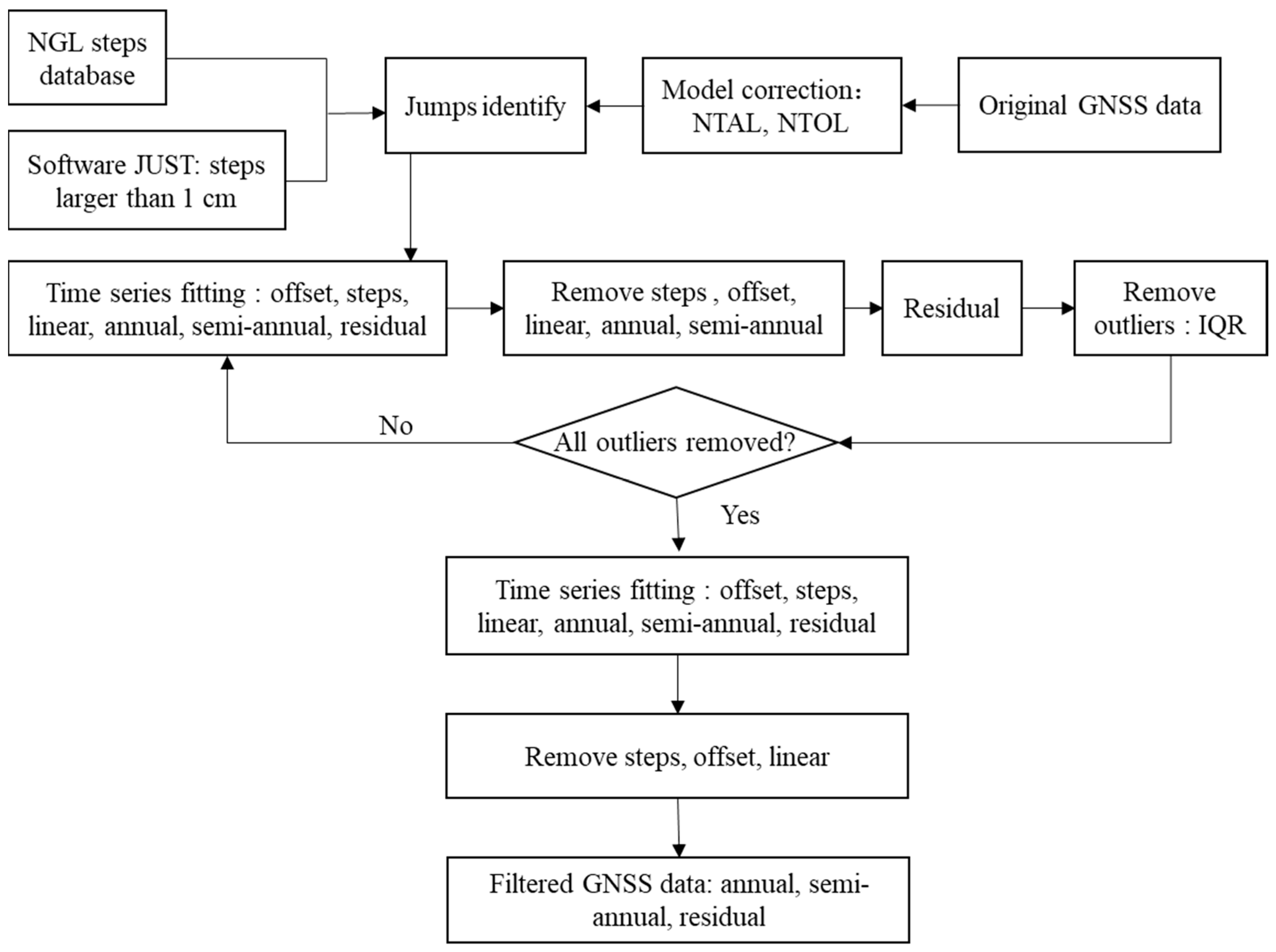
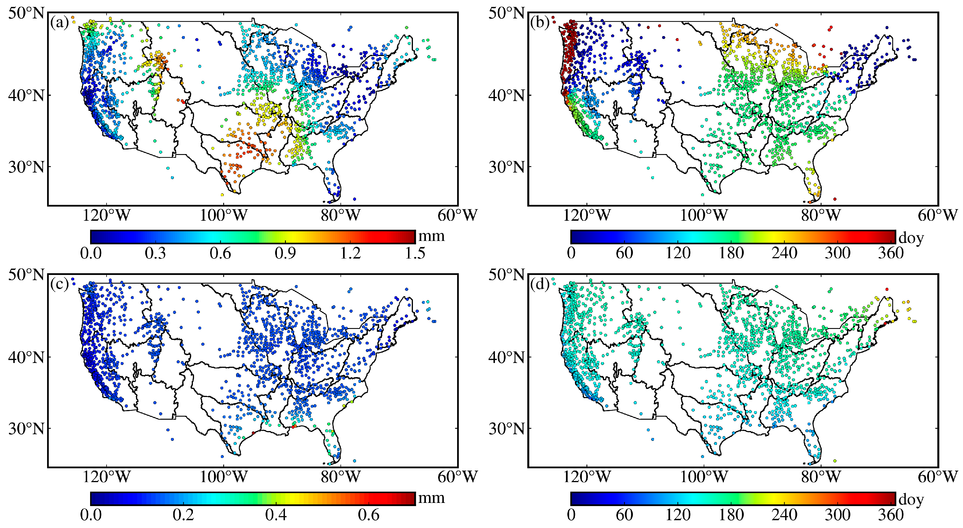
2.2.1. GNSS Vertical Displacements

We collect daily GNSS station time series and the corresponding standard deviations (STDs) released by the Nevada Geodetic Laboratory (NGL) in the International GNSS Service 2014 reference frame from 1 January 2018 to 31 August 2022 [37], in order to be consistent with the GFO observation span. The GNSS time series were processed with GipsyX software-1.0 [38]; details of the GNSS data analysis strategies are available on the NGL website (http://geodesy.unr.edu/gps/ngl.acn.txt, accessed on 18 December 2022). We use the GNSS stations selected by Argus et al. [39]. Following their recommendations, we remove the GNSS sites affected by volcanic activity in California, as well as those influenced by solid Earth’s porous responses due to groundwater withdrawal in California and oil extraction in the Gulf Coast, which are the two most prominent aquifer systems across the CONUS [40]. We remove the GNSS stations whose displacements are out of phase with the nearby stations [27,41,42] and the stations with observation durations of less than 2 years. Finally, 1437 GNSS stations are employed to study the TWS changes across the CONUS. The distribution and continuity of GNSS stations and total number of GNSS stations recorded each day are shown in Figure 2b, c. The area and number of GNSS stations of the 18 watersheds and the CONUS are listed in Table 1. Figure 3 shows the flow chart of the GNSS data processing process.

Surface displacements induced by non-linear variations, such as non-tidal atmospheric loading (NTAL) and non-tidal oceanic loading (NTOL), are unrelated to hydrological loading and need to be eliminated from the GNSS time series [43,44]. To isolate hydrological loading, we remove the vertical displacements due to NTAL and NTOL at each GNSS station. NTAL and NTOL can be downloaded from the Earth System Modeling group at Deutsches GeoForschungsZentrum [45]. We fit the vertical displacements caused by NTAL and NTOL with Equation (1) using the least squares method, as shown in Figure 4; the amplitudes of the annual terms in vertical displacements induced by NTAL and NTOL are 0~1.5 mm and 0~0.7 mm, respectively.

$$\mathrm{y}\left(t\right)=A+Bt+Ccos\left(wt+{\theta }_1\right)+Dcos\left(2wt+{\theta }_2\right)+\epsilon$$

(1)

where $t$ represents the epoch with a daily or monthly resolution; $y$ represents vertical displacement or TWS; $A$ represents the offset; $B$ represents the linear trend, $C,D,{ \theta }_1,$ and ${\theta }_2$ represent the amplitudes and phases of annual and semi-annual components; and $\epsilon$ represents a residual.

We fit the GNSS time series with the following equation:

$$\mathrm{y}\left(t\right)=A+Bt+Ccos\left(wt+{\theta }_1\right)+Dcos\left(2wt+{\theta }_2\right)+\sum _{i=1}^k{E}_{i}H\left(t-{tE}_i\right)+\epsilon$$

(2)

where $t$ represents the epoch with daily resolution; $y$ represents GNSS vertical displacement; $A$ represents the offset; $B$ represents the linear trend; $C,D,{\theta }_1,$ and ${\theta }_2$ represent the amplitudes and phases of annual and semi-annual components; $E$ represents the step caused by earthquakes, equipment replacement, and so on, at the $tE$ epoch; $\epsilon$ represents the residual; and $H$ represents the Heaviside function, which is 0 and 1 when $(t-{tE}_i)$ is negative and positive, respectively. The main steps in the GNSS time series can be found in the database on the NGL website (http://geodesy.unr.edu/NGLStationPages/steps.txt, accessed on 30 December 2022); potential jumps with a threshold of 1 cm in the GNSS time series are identified using change detection and time series analysis software, jumps upon spectrum and trend (JUST) [46].

The outliers in each GNSS time series are detected and omitted based on the median and interquartile range (IQR) statistics [47]. Within a sliding window centered on the GNSS displacement corresponding to each epoch, the median and IQR are calculated. When the difference between the residual and the median is 3 times larger than the IQR, it is automatically determined as an outlier.

$$\mid v_i-median\left(v_{i-\frac{L}{2},i+\frac{L}{2}}\right)\mid >3·IQR\left(v_{i-\frac{L}{2},i+\frac{L}{2}}\right)$$

(3)

where $v_i$ represents the ith residual in the GNSS time series, $L$ represents the length of the sliding window, which is set to be 1 year, and the window gradually slides with each epoch as the center of the window.

We first extract the residual term using Equation (2), and then remove the outliers using Equation (3) for each GNSS time series; all the outliers are omitted after several iterations. Finally, we remove the offset, linear trend, and steps in the GNSS time series. The resulting signals mainly reflect hydrological loading deformation, including the seasonal and residual terms in Equation (2). Figure 5 shows the GNSS vertical displacements time series at six selected stations; after the iterations mentioned above are performed, the steps are easily identified, and the outliers are effectively removed.

2.2.2. GFO Time-Variable Solutions

We use the GFO RL06 mascon data released by the Center for Space Research (CSR) at the University of Texas at Austin [48] from May 2018 to August 2022. The CSR mascon solutions are estimated on a hexagonal geodesic grid and have a spatial sampling of about 1° in equatorial longitude and a monthly temporal resolution, limited by the band-limited nature; the 1° spatial sampling is likely not the spatial resolution of the GRACE solutions, and the spatial resolution is about 300−500 km [49]. The CSR mascon solutions reflect changes in the TWS, and they are expressed in terms of the equivalent water height (EWH). During generation, the CSR mascons are corrected for glacial isostatic adjustment and leakage effects. Note that the low-degree changes (e.g., degree-one, C20, and C30) are resolved with independent measurements or models [50,51].

2.2.3. Hydrological Models

The Global Land Data Assimilation System (GLDAS) [52] Noah2.1 model provides 4-layered soil moisture values of 0~2 m below the surface and snow water content data on the Earth’s surface. We integrate soil moisture and snow water in the estimation of the shallow-surface TWS (GLDAS-TWS). We use three sets of GLDAS hydrological models with different spatial resolutions. The monthly models with a grid interval of 1° from January 2020 to December 2020 are used to simulate the vertical deformations at each GNSS station across the CONUS. The monthly models with a grid interval of 0.25° from January 2018 to August 2022 are used to evaluate the consistency of the TWS estimated using the GNSS (GNSS-TWS) and TWS derived with GFO (GFO-TWS). The models with a temporal resolution of 3 h and grid interval of 0.25° from 1 January 2019 to 31 January 2019 are used to extract daily shallow-surface TWS variations caused by a heavy precipitation event in January 2019 in the California watershed.

2.2.4. Meteorological Precipitation Products

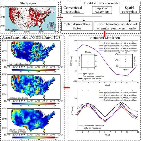
We adapt reconstructed monthly precipitation datasets from January 2018 to August 2022 provided by National Oceanic and Atmospheric Administration (NOAA) for the estimation of precipitation over the CONUS. The datasets are provided in the format of 0.5° × 0.5° grids at a global scale and are derived from a network of global gauge stations by employing advanced interpolation techniques to fill in the missing data [53]. The daily datasets are available in the format of 0.25° × 0.25° grids over the CONUS and are constructed using an interpolation algorithm based on gauge observations collected from multiple sources [54,55].

3. Methodology

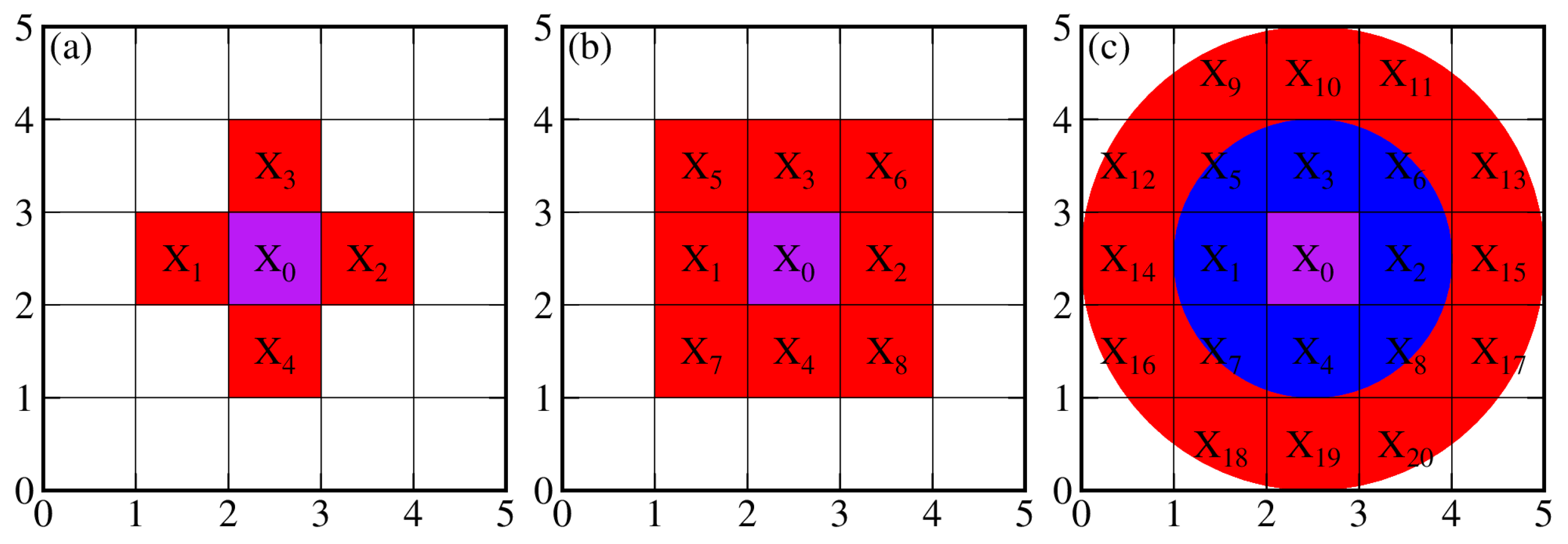
3.1. GNSS Inversion Method

According to the elastic deformation theory [5,28,56,57], the relationship between vertical displacements and TWS in the EWH reads:

$$L+v=Gx$$

(4)

where $L$ represents the vertical displacements measured by GNSS, $v$ represents the observation residual, $G$ represents Green’s function calculated based on the disc model [7,8], and $x$ represents TWS to be estimated for each grid cell; the study area is divided into a 1° × 1° grid cell. In order to mitigate the edge effects, we extend the study area by 2.5° and 0.5° beyond the land and ocean, respectively. The number of grid cells is less than the number of GNSS sites in this study; therefore, the inversion solutions are overdetermined problems. Equation (4) is subject to this condition:

$${‖Pv‖}^2\to min$$

(5)

where P represents the diagonal weight matrix, which is constructed using the inverse of the variance in GNSS vertical displacements. Equation (5) is ill-posed when the number of grid cells is larger than the number of GNSS stations; the Tikhonov regularization method is commonly used for solving ill-posed equations [58]. In addition, to ensure smooth spatial variations in the TWS between adjacent grid cells, a regularization term like Tikhonov is added to Equation (4). The constraint based on the Laplacian operator is as follows [59]:

$$\lambda Dx=0$$

(6)

where $\lambda$ represents the smoothing factor that adjusts the relative weight between the model misfit and roughness. $D$ represents the Laplacian operator with the following kernels:$\left[ \begin{array}{ccc}0& 1& 0\\ 1& -4& 1\\ 0& 1& 0\end{array}\right]$. Thus, Equation (5) is written as follows after adding the Laplacian constraints:

$${‖Pv‖}^2+{\lambda }^2{‖Dx‖}^2\to min$$

(7)

where the first term ${‖Pv‖}^2$ represents the model misfit, and the second term ${‖Dx‖}^2$ represents the roughness of the solution. The TWS is estimated as follows:

$$x={{(G}^{T}PG+\lambda D^{T}D)}^{-1}{G}^{T}PL$$

(8)

In addition to the Laplacian constraint strategy mentioned above, the conventional constraint strategy is also applied in this study, which is similar to the Laplacian constraints in Equation (6), but the Laplacian operator is replaced with the identity matrix. The conventional constraint strategy addresses the issue of ill-posed equations but does not consider the smoothness of the TWS changes between adjacent grid cells. The formula is as follows:

$$\lambda Ix=0$$

(9)

where $I$ represents the identity matrix. The TWS is inverted as follows:

$$x={{(G}^{T}PG+\lambda I)}^{-1}{G}^{T}PL$$

(10)

The optimal smoothing factors need to be determined before inversion for the conventional constraints and Laplacian constraints. We use the GCV approach to estimate the optimal parameters. We utilize the GNSS vertical displacements from 1 January 2018 to 31 August 2022 at 1437 GNSS stations across the CONUS and run the inversion with various values of $\lambda$. Subsequently, we obtain the curves between the smoothing factors and the sum of squared residuals obtained through cross-validation (CVSS). As shown in Figure 6, the optimal parameters are 3.2 for conventional constraints and 1.3 for Laplacian constraints, as in these cases, the CVSS values are minimized.

As mentioned above, the principle of spatial constraints is as follows: the absolute difference between the EWH of the $k$th grid cell and the average EWH of all the grid points in the circle with a radius of $r$ centered on the $k$th grid cell is within a certain range. This is illustrated by the following inequality:

$$|x_k-\frac{1}{n}(x_{k_1}+x_{k_2}+\cdots +x_{k_n})|\le e$$

(11)

where $x_k$ represents the EWH of the kth grid cell; $x_{k_1}, x_{k_2}, \cdots , x_{k_n}$ represent the EWH of all the grid points within a circle of radius r centered on the kth grid cell; and e represents the set threshold value. Equation (11) is the same as the following inequality:

$$\left|Ax\right|\le e$$

(12)

where A represents the constraint matrix.

The above inequality is transformed into an equality below, and then a non-linear programming approach is utilized to solve it by introducing the vector $y (0\le y\le 2e)$.

$$Ax+y=e$$

(13)

By combining Equations (5) and (13), the following equation for TWS inversion under spatial constraints is established:

$$\begin{gathered} {‖Pv‖}^2\to min \\ \mathrm{s}.\mathrm{t}. Ax+y=e \end{gathered}$$

(14)

where x and y are the parameters that need to be estimated. Equation (14) can be written as follows:

$$\begin{gathered} {‖P(\left[\begin{array}{cc}G& 0\end{array}\right]·\left[\begin{array}{c}x\\ y\end{array}\right]-L)‖}^2\to min \\ \mathrm{s}.\mathrm{t}. \left[\begin{array}{cc}A& I\end{array}\right]·\left[\begin{array}{c}x\\ y\end{array}\right]=e \end{gathered}$$

(15)

We use MATLAB’s lsqlin routine to solve Equation (15) following Khorrami et al. [60], which represents a constrained least squares adjustment. We choose the ‘interior-point’ algorithm in the lsqlin routine, where the lower and upper bounds of x are set to be −0.5 m and 0.5 m, respectively, the lower and upper bounds of y are set to be 0 and $2·\mathrm{e}$, respectively, and the initial points of x and y are set to be 0. Then, the two unknown parameters x and y are solved.

3.2. Closed-Loop Simulation

We conduct a closed-loop simulation to assess the performance of spatial constraints for recovering the TWS variations. The procedure is described as follows: Firstly, we extract soil moisture and snow water data from the monthly GLDAS 1° × 1° dataset in 2020 across the CONUS, which is used as the input signal. Next, we forward calculate the monthly vertical displacements at each GNSS station. The noise signals at each GNSS station are obtained by averaging the STD of vertical displacements from 1 January 2020 to 31 December 2020 in each month. Then, we apply different constraint strategies to invert the monthly spatial distributions of the TWS and obtain the TWS time series. Finally, we calculate the amplitudes and STDs of monthly TWS from the conventional (CC-TWS), Laplacian (LC-TWS), and spatial constraints (SC-TWS).

For the spatial constraint inversion algorithm, two empirical parameters, the radius r and the threshold e, jointly control the spatial smoothness of the TWS variations, which, in turn, affects the oscillation amplitude of the TWS time series. We illustrate the performance of the spatial constraints in TWS inversion using different combinations of r and e (see

Table 2. Annual amplitudes of input GLDAS and recovered TWS and average STDs between input GLDAS and recovered TWS across the CONUS in 2020. CC and LC represent conventional and Laplacian constraints, respectively. The first three digits and the last two digits after the letter SC represent the values of the parameters r and e of the spatial constraint inversion method, respectively. For example, SC15045 represents the parameters r = 150 km, e = 45 mm, and so on.

Constraint Strategy	Amplitude (mm)	Average STDs (mm)
input	52.59
CC	50.06	14
LC	50.21	14
SC15045	51.03	11
SC20045	50.76	12
SC25055	50.74	11
SC30060	50.82	11
SC35065	50.76	11
SC40060	50.68	13
SC45075	51.00	12
SC50075	50.89	12

). The amplitudes and average STDs are shown in Table 2, the average STDs of the SC-TWS are lower than those of the CC-TWS and LC-TWS, indicating that the spatial constraint inversion results are closer to the input TWS. The conventional constraints exhibit the minimum oscillation amplitude, and the spatial constraints show the maximum oscillation amplitude.

We use the following equation to quantify the improvement of TWS using the spatial constraint method:

$$∆\mathrm{S}\mathrm{T}\mathrm{D}=\frac{{\mathrm{S}\mathrm{T}\mathrm{D}}_{\mathrm{C}\mathrm{C}/\mathrm{L}\mathrm{C}}-{\mathrm{S}\mathrm{T}\mathrm{D}}_{\mathrm{S}\mathrm{C}}}{{\mathrm{S}\mathrm{T}\mathrm{D}}_{\mathrm{C}\mathrm{C}/\mathrm{L}\mathrm{C}}}\times 100\%$$

(16)

where ${\mathrm{S}\mathrm{T}\mathrm{D}}_{\mathrm{C}\mathrm{C}/\mathrm{L}\mathrm{C}}$ represents the average STDs of the conventional or Laplacian constraints, ${\mathrm{S}\mathrm{T}\mathrm{D}}_{SC}$ represents the average STDs of the spatial constraints, and $∆\mathrm{S}\mathrm{T}\mathrm{D}$ represents the improvement of the spatial constraint method. From Table 2, we can see that the spatial constraint inversion is improved by 7–21% compared with the inversion using the conventional and Laplacian constraints.

4. Results and Analysis

4.1. Spatial Distributions of TWS

We recover the daily TWS variations across the CONUS with a 1° grid using three inversion strategies and evaluate their spatial patterns by comparing them to the patterns from the GFO-TWS, GLDAS, and precipitation dataset. We fit the daily TWS time series with Equation (1) using the least squares method at each grid cell and obtain the annual amplitudes. We select the following set of parameters to illustrate the spatial constraint inversion performance: r = 300 and e = 60 (SC30060), as they are one of the parameter sets that exhibit good performance in the closed-loop simulation (Table 2). As shown in Figure 7, the spatial distributions of the annual amplitude from various data sources are consistent over many regions. In general, the CC-TWS exhibits the largest amplitude, the SC-TWS displays the smallest amplitude, and the LC-TWS approximately falls between the two in terms of amplitude. The amplitudes of the annual terms in the CC-TWS and LC-TWS exhibit a rougher texture in the spatial domain, resulting in larger amplitudes. Conversely, the SC-TWS shows a smoother spatial distribution of annual amplitudes. The strong signals are mainly distributed in the watersheds of lower Mississippi, the Pacific Northwest, and California. We investigate the spatial distributions of the TWS for r and e listed in Table 2 for spatial constraint inversion. As shown in Figure 8, the TWS exhibits consistent spatial distributions across various parameter settings. This result implies that the spatial constraint inversion is less sensitive to the changes in the parameters of r and e, it can provide us a robust inversion with a more flexible range of parameter combinations.

The spatial distribution of the annual amplitudes from the LC-TWS and SC-TWS presents some discrepancies in several regions compared with the GFO, GLDAS, and precipitation (Figure 7), e.g., in the Rio Grande watershed region, we observe apparent TWS signals in the inversion using spatial constraints, but those signals are not seen in the LC-TWS and CC-TWS, and neither GFO nor GLDAS show similar signal patterns. We speculate that this discrepancy could be due to the sparse GNSS stations in this region, and therefore the spatial constraints might introduce some unrealistic signals. In addition, we find evident discrepancies in the watersheds of New England and South Atlantic–Gulf, which may be attributed to the local climate characteristics; another reason could be that GNSS is more sensitive to local mass loading, while the GFO is sensitive to large-scale mass changes.

We compare the TWS variations with precipitation (Figure 7). Precipitation mainly concentrates in the southeast and northwest of the CONUS; the average annual precipitation total is 1000–2500 mm. The large oscillations of the GLDAS, GFO, and GNSS-TWS in the Pacific Northwest watershed region are caused by abundant precipitation. In addition, abundant precipitation causes an obvious increase in the GLDAS, GFO, and GNSS-TWS values around the Appalachian Mountains due to the good water and soil conservation effects. While the oscillation of TWS is weak far from the Appalachian Mountains, this is attributed to the precipitation in flat areas flowing into the Atlantic Ocean through rivers.

4.2. Temporal Variation Features of TWS

We assess the temporary variations in the TWS for all the watersheds (Figure 9). The watershed mean TWS variations are computed using a cosine latitude weighting scheme. We focus on the monthly mean changes; therefore, we average the daily time series into a monthly time series. The TWS variations in the CONUS vary significantly over time in different regions. Figure 9 shows the monthly TWS time series from January 2018 to August 2022 in the 18 watersheds and the CONUS. As shown in Figure 9, the time series variations in the CC-TWS, LC-TWS, and SC-TWS are generally consistent, indicating that the impact of different constraints strategies on the TWS time series is minor over regional scales. The temporal variations in the GNSS-TWS, GFO-TWS, and GLDAS-TWS are consistent, particularly in the regions with large oscillation amplitudes, such as the watersheds of lower Mississippi, the Pacific Northwest, and California. However, it is inconsistent in the Rio Grande watershed due to the fact that the GNSS stations are sparsely distributed.

We compare the annual amplitudes of the GNSS-TWS with the GFO-TWS and GLDAS-TWS to quantitatively evaluate the performance of the GNSS inversion strategies. The TWS time series mainly show seasonal variations; therefore, we fit the TWS time series using Equation (1) and obtain the amplitudes of the annual terms in the TWS time series for each watershed. As shown in

Table 3. The amplitudes of the annual terms in GNSS-TWS, GFO-TWS, and GLDAS-TWS time series. CC and LC represent conventional and Laplacian constraints, respectively. SC30060 represents the parameters r = 300 km and e = 60 mm for spatial constraints.

HUC-2	Amplitude (mm)
	CC	LC	SC30060	GFO	GLDAS
1	28.76 ± 8.79	30.41 ± 9.21	41.74 ± 8.79	97.23 ± 9.02	111.64 ± 6.08
2	45.15 ± 7.75	45.78 ± 8.21	39.64 ± 7.93	43.44 ± 8.81	66.71 ± 5.58
3	20.48 ± 7.39	25.64 ± 7.83	27.00 ± 8.44	55.28 ± 7.58	39.98 ± 5.47
4	14.14 ± 10.62	13.09 ± 10.90	10.73 ± 11.07	24.39 ± 11.65	87.47 ± 5.09
5	37.62 ± 6.02	38.29 ± 5.81	35.42 ± 5.61	80.32 ± 4.35	79.47 ± 4.60
6	79.22 ± 14.62	75.02 ± 13.72	63.71 ± 10.42	107.65 ± 6.91	86.12 ± 5.93
7	28.14 ± 8.57	26.43 ± 7.74	26.56 ± 7.87	62.72 ± 7.64	53.78 ± 7.87
8	94.58 ± 10.85	106.70 ± 11.71	96.79 ± 11.40	133.45 ± 10.23	86.09 ± 7.11
9	51.49 ± 9.93	72.96 ± 10.38	71.22 ± 11.01	40.26 ± 9.78	39.88 ± 9.19
10	33.52 ± 7.94	36.08 ± 9.44	37.14 ± 8.86	47.08 ± 8.32	25.94 ± 4.52
11	26.39 ± 9.45	13.89 ± 12.10	23.72 ± 11.33	58.11 ± 7.49	36.97 ± 6.96
12	38.58 ± 11.52	37.23 ± 11.68	30.87 ± 11.80	41.84 ± 8.72	30.56 ± 8.37
13	18.90 ± 4.97	39.68 ± 12.52	88.14 ± 10.78	17.38 ± 7.24	4.41 ± 2.84
14	34.14 ± 7.32	48.91 ± 10.89	62.10 ± 9.78	59.90 ± 5.83	26.94 ± 3.09
15	27.27 ± 6.99	72.49 ± 12.95	47.36 ± 10.53	28.36 ± 5.90	12.19 ± 3.38
16	15.72 ± 9.64	26.19 ± 10.39	11.81 ± 9.89	58.31 ± 7.41	42.84 ± 3.16
17	94.74 ± 9.06	96.90 ± 9.12	89.12 ± 8.86	113.62 ± 3.59	119.56 ± 3.70
18	54.43 ± 11.38	58.79 ± 11.64	56.38 ± 12.05	81.63 ± 8.81	86.97 ± 5.07
CONUS	22.28 ± 5.78	21.55 ± 6.09	21.13 ± 6.10	60.65 ± 4.55	51.61 ± 3.03

, the CC-TWS, LC-TWS, and SC-TWS exhibit amplitudes that are comparable to those of the GFO-TWS and GLDAS-TWS in most of the watersheds. However, we find that the amplitudes of the annual term in the SC-TWS is nearly four times larger than the GFO-TWS in the Rio Grande watershed, probably due to the sparse distribution of GNSS stations. The amplitudes of the annual terms in the CC-TWS, LC-TWS, and SC-TWS are about 0.3 times larger than those in the GFO-TWS in the Great Basin watershed; this large discrepancy may be due to tectonic activity and climate types, and the GNSS vertical displacements may be contaminated by non-hydrological factors. We calculate the STDs of the time series between the GNSS-TWS and GFO-TWS in order to quantify the consistency of the TWS inverted from various constraints strategies and the GFO. As shown in

Table 4. The STD between time series of GNSS-TWS and GFO-TWS. CC and LC represent conventional and Laplacian constraints, respectively. SC30060 represents the parameters r = 300 km and e = 60 mm for spatial constraints.

HUC-2	STD (mm)
	CC	LC	SC30060
1	69	70	65
2	55	57	55
3	51	53	55
4	46	48	47
5	40	38	39
6	86	78	57
7	57	56	54
8	51	47	51
9	45	54	54
10	41	42	42
11	48	53	47
12	61	63	56
13	47	83	87
14	46	64	53
15	43	82	64
16	64	72	64
17	54	55	54
18	64	63	65
CONUS	37	37	38

, the STDs of the SC-TWS across 13 watersheds are smaller than those of the LC-TWS. The STDs of the SC-TWS and LC-TWS are at the same level, and the deviations are within 5 mm in the remaining five watersheds and the CONUS.

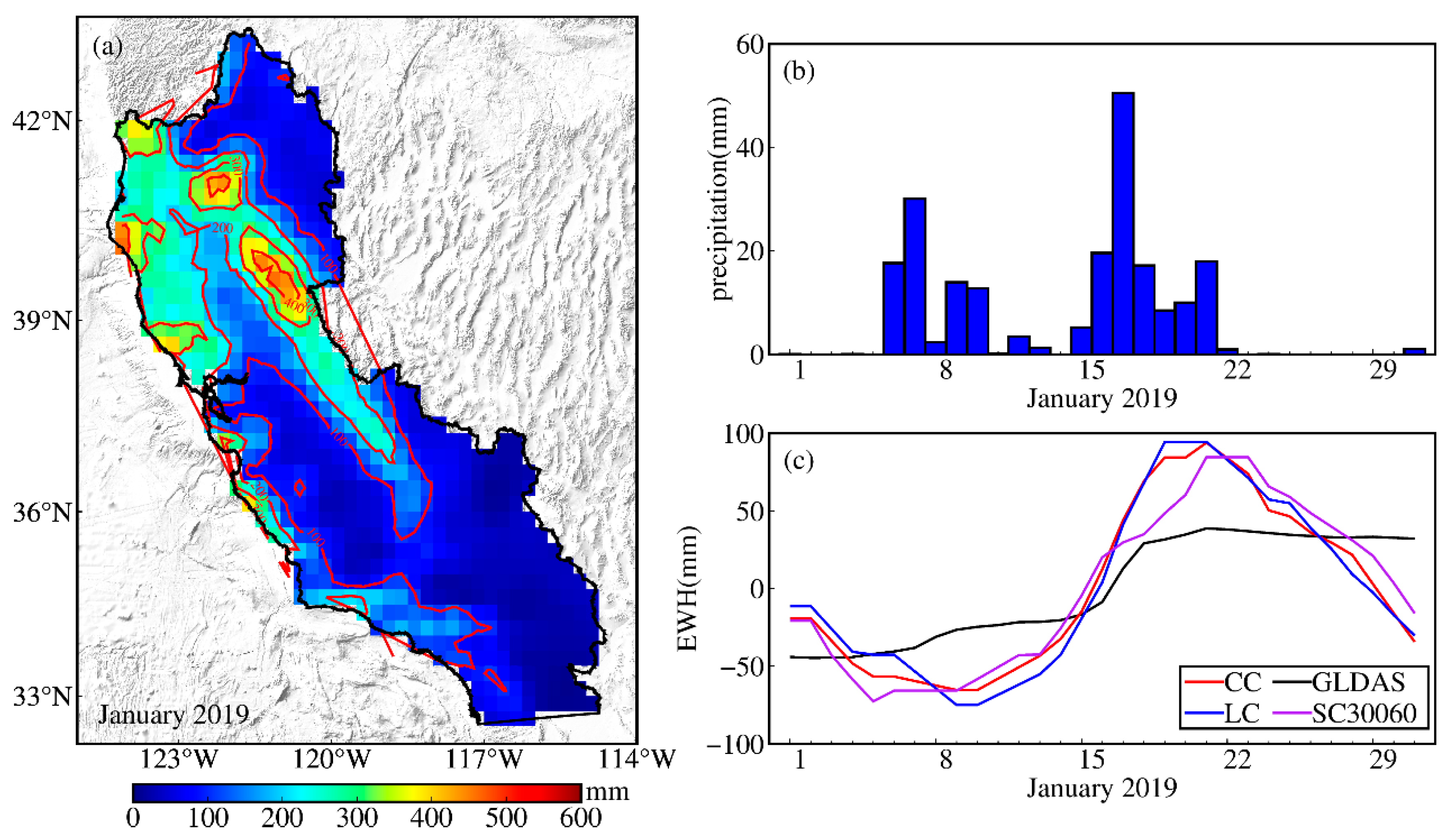
4.3. Identifying Extreme Precipitation Events in the California Watershed

The GNSS has great advantages in capturing instantaneous high-frequency signals due to its high temporal resolution, e.g., Milliner et al. successfully tracked the daily transient TWS caused by hurricane Harvey based on the vertical and horizontal GNSS displacements in Gulf Coast of the CONUS [33]. Jiang et al. confirmed that the GNSS could be used to track a stormwater event in Yunnan, China, which was weaker than the catastrophic storm surges [17].

We investigate the TWS change caused by extreme precipitation in January 2019 in the California watershed. We obtain the spatial distribution of the monthly precipitation total, daily time series of precipitation, GNSS-TWS, and GLDAS-TWS in the California watershed in January 2019. As shown in Figure 10, precipitation is mainly concentrated around California’s Central Valley and the western Pacific coastal area, the total of which is lower in the northeast and southeast inland areas of California. The maximum precipitation total is 460 mm in the northwest of California’s Central Valley in January 2019. We calculate the daily precipitation time series of the grid points with a total precipitation greater than 100 mm, which shows that California experienced two extreme precipitation events in January 2019; the first extreme precipitation event lasted five days from 6 January to 10 January, with the maximum average precipitation reaching 30 mm on 7 January, and the second extreme precipitation event lasted six days from 16 January to 21 January, with the maximum average precipitation reaching 51 mm on January 17. In order to reduce the noise, we fit the daily GNSS-TWS time series with a 7 day median and a 3 day moving average filter, and the GNSS-TWS increased rapidly after the first extreme precipitation event. The GNSS-TWS reached the maximum immediately due to the continuous accumulation of precipitation after the second extreme precipitation event. The GNSS-TWS remained stable change for about 3 days after the two extreme precipitation events. The evolution of the daily GLDAS-TWS is consistent with that of the GNSS-TWS, while the amplitude of the GLDAS-TWS is smaller than the GNSS-TWS. The correlation coefficients of the CC-TWS, LC-TWS, SC-TWS, and GLDAS-TWS are 0.82, 0.78, and 0.82, respectively. This demonstrates that spatial constraint inversion can be an independent constraint strategy used to extract the TWS caused by extreme precipitation events.

5. Discussion and Conclusions

The spatial constraints provide a valuable complement to the existing conventional and Laplacian constraint methods. The inversion results with spatial constraints are subject to two important parameters (i.e., the radius r and the threshold e). The parameter e determines to what extent the spatial pattern will be smoothed, and the parameter r affects the spatial scale that will be constrained. Our work suggests that there is no need to precisely estimate the optimal parameters for spatial constraints; instead, a rough range for the empirical parameters is sufficient. As shown in Figure 8, changes in these two factors do not necessarily cause dramatically different inversion results; for instance, the evident signal in the northwest region is similar for different combinations of r and e. The spatial constraints allow us to employ a more flexible range of parameter selection, but still provide robust inversion results.

The densely distributed continuous GNSS stations across the CONUS enable us to study land–water cycle processes with a high spatiotemporal resolution. The constraints are effective in most regions, and the spatiotemporal distribution of the TWS from the GNSS is consistent with those of the GFO and GLDAS. We illustrate the performance of spatial constraints using the six sets of parameters listed in Table 2 and compare the results with conventional and Laplacian constraints. As the spatial distribution of the TWS is not sensitive to changes in the two empirical parameters, the range of parameters for the spatial constraints is not limited to these six sets. The parameters r and e fluctuate within a certain range, and the TWS inversion results remain stable, allowing a broader range of r and e values. We can apply the spatial constraint inversion method with flexible parameter selection to other regions with a dense distribution of GNSS stations, such as Europe and Japan.

The TWS variations inferred from the GNSS vertical displacements using the spatial constraint inversion method still face some challenges and limitations. The GNSS vertical displacement time series contains all the land motion signals, and the unmodelled vertical deformation caused by thermal expansion of the monument [61] also affects the isolation of the hydrological loading, which is difficult to accurately separate. Our proposed method only applies flexible spatial constraints, but it cannot reduce the noise in the GNSS measurements. Without doubt, using a preprocessing strategy to denoise the GNSS measurements would improve the inversion not only using the spatial constraints but also using other methods. In addition, using the STDs to evaluate the inversion also has limitations, especially in the inversion with real GNSS data, because the true TWS signal is unknown. In our evaluation, we assume that the signals observed with GRACE/GFO are true; therefore, a small difference in GRACE/GFO would indicate a better result. However, we must recognize that, on the one hand, the TWS variations observed with GRACE/GFO suffer from a low resolution, and on the other hand, they reflect total variations, including the changes in groundwater, which may not be well observed by GNSS measurements.

With the increase in global temperatures, droughts and floods are more frequent, severe, and longer lasting [62]. The use of GNSS observations for studying the loading deformation caused by extreme hydrological events, such as storms, hurricanes, and heavy precipitation, will become increasingly important. It is of great significance to conduct research on the inversion of the TWS. The improvement in GNSS data processing and the enrichment of the GNSS inversion methods will better serve meteorological and hydrological management departments in the future.

We propose a new inversion method with flexible spatial constraints for daily TWS inversion using the GNSS vertical displacements from January 2018 to August 2022 across the CONUS in this study. Our closed-loop simulation demonstrates that the spatial constraint inversion has an advantage in recovering the annual oscillation amplitude of the TWS. Additionally, the TWS time series from spatial constraints are closer to the input signals. We use conventional, Laplacian, and spatial constraints to investigate the spatiotemporal distributions of the TWS across the CONUS and compare them with the GFO-TWS and GLDAS-TWS. The results show that the spatial distributions of the annual amplitude from different constraint strategies are consistent with those of the GFO and GLDAS over many regions, but still present some discrepancies in the regions with sparse GNSS stations. The temporal variations in GNSS-TWS from different constraint strategies show good consistency with GFO and GLDAS, and the STDs between SC-TWS, LC-TWS and GFO are at the same level. The spatial constraint inversion proposed in this study can be an alternative tool for TWS inversion.

References

1. Fu, Y.; Argus, D.F.; Landerer, F.W. GPS as an independent measurement to estimate terrestrial water storage variations in Washington and Oregon. J. Geophys. Res. Solid Earth 2015, 120, 552–566. [Google Scholar] [CrossRef]
2. White, A.M.; Gardner, W.P.; Borsa, A.A.; Argus, D.F.; Martens, H.R. A review of GNSS/GPS in hydrogeodesy: Hydrologic loading applications and their implications for water resource research. Water Resour. Res. 2022, 58, e2022WR032078. [Google Scholar] [CrossRef] [PubMed]
3. Tapley, B.D.; Watkins, M.M.; Flechtner, F.; Reigber, C.; Bettadpur, S.; Rodell, M.; Sasgen, I.; Famiglietti, J.S.; Landerer, F.W.; Chambers, D.P.; et al. Contributions of GRACE to understanding climate change. Nat. Clim. Chang. 2019, 9, 358–369. [Google Scholar] [CrossRef] [PubMed]
4. Argus, D.F.; Fu, Y.; Landerer, F.W. Seasonal variation in total water storage in California inferred from GPS observations of vertical land motion. Geophys. Res. Lett. 2014, 41, 1971–1980. [Google Scholar] [CrossRef]
5. Argus, D.F.; Landerer, F.W.; Wiese, D.N.; Martens, H.R.; Fu, Y.; Famiglietti, J.S.; Thomas, B.F.; Farr, T.G.; Moore, A.W.; Watkins, M.M. Sustained water loss in California’s mountain ranges during severe drought from 2012 to 2015 inferred from GPS. J. Geophys. Res. Solid Earth 2017, 122, 10559–10585. [Google Scholar] [CrossRef]
6. Borsa, A.A.; Agnew, D.C.; Cayan, D.R. Ongoing drought-induced uplift in the western United States. Science 2014, 345, 1587–1590. [Google Scholar] [CrossRef]
7. Farrell, W.E. Deformation of the Earth by surface loads. Rev. Geophys. 1972, 10, 761–797. [Google Scholar] [CrossRef]
8. Wahr, J.; Khan, S.A.; van Dam, T.; Liu, L.; van Angelen, J.H.; van den Broeke, M.R.; Meertens, C.M. The use of GPS horizontals for loading studies, with applications to northern California and southeast Greenland. J. Geophys. Res. Solid Earth 2013, 118, 1795–1806. [Google Scholar] [CrossRef]
9. Zhang, T.; Jin, S. Evapotranspiration variations in the Mississippi river basin estimated from GPS observations. IEEE Trans. Geosci. Remote Sens. 2016, 54, 4694–4701. [Google Scholar] [CrossRef]
10. Enzminger, T.L.; Small, E.E.; Borsa, A.A. Accuracy of snow water equivalent estimated from GPS vertical displacements: A synthetic loading case study for western U.S. mountains. Water Resour. Res. 2018, 54, 581–599. [Google Scholar] [CrossRef]
11. Enzminger, T.L.; Small, E.E.; Borsa, A.A. Subsurface water dominates Sierra Nevada seasonal hydrologic storage. Geophys. Res. Lett. 2019, 46, 11993–12001. [Google Scholar] [CrossRef]
12. Shen, Y.; Yan, H.; Peng, P.; Feng, W.; Zhang, Z.; Song, Y.; Bai, X. Boundary-included enhanced water storage changes inferred by GPS in the Pacific rim of the western United States. Remote Sens. 2020, 12, 2429. [Google Scholar] [CrossRef]
13. Zhang, B.; Yao, Y.; Fok, H.S.; Hu, Y.; Chen, Q. Potential seasonal terrestrial water storage monitoring from GPS vertical displacements: A case study in the lower three-rivers headwater region, China. Sensors 2016, 16, 1526. [Google Scholar] [CrossRef] [PubMed]
14. Hsu, Y.-J.; Fu, Y.; Bürgmann, R.; Hsu, S.-Y.; Lin, C.-C.; Tang, C.-H.; Wu, Y.-M. Assessing seasonal and interannual water storage variations in Taiwan using geodetic and hydrological data. Earth Planet. Sci. Lett. 2020, 550, 116532. [Google Scholar] [CrossRef]
15. Lai, Y.R.; Wang, L.; Bevis, M.; Fok, H.S.; Alanazi, A. Truncated singular value decomposition regularization for estimating terrestrial water storage changes using GPS: A case study over Taiwan. Remote Sens. 2020, 12, 3861. [Google Scholar] [CrossRef]
16. Zhong, B.; Li, X.; Chen, J.; Li, Q.; Liu, T. Surface mass variations from GPS and GRACE/GFO: A case study in southwest China. Remote Sens. 2020, 12, 1835. [Google Scholar] [CrossRef]
17. Jiang, Z.; Hsu, Y.-J.; Yuan, L.; Huang, D. Monitoring time-varying terrestrial water storage changes using daily GNSS measurements in Yunnan, southwest China. Remote Sens. Environ. 2021, 254, 112249. [Google Scholar] [CrossRef]
18. Shen, Y.; Zheng, W.; Yin, W.; Xu, A.; Zhu, H.; Yang, S.; Su, K. Inverted algorithm of terrestrial water-storage anomalies based on machine learning combined with load model and its application in southwest China. Remote Sens. 2021, 13, 3358. [Google Scholar] [CrossRef]
19. Liu, B.; Yu, W.; Dai, W.; Xing, X.; Kuang, C. Estimation of terrestrial water storage variations in Sichuan-Yunnan region from GPS observations using independent component analysis. Remote Sens. 2022, 14, 282. [Google Scholar] [CrossRef]
20. Li, X.; Zhong, B.; Li, J.; Liu, R. Inversion of terrestrial water storage changes from GNSS vertical displacements using a priori constraint: A case study of the Yunnan province, China. J. Hydrol. 2023, 617, 129126. [Google Scholar] [CrossRef]
21. Han, S.-C.; Razeghi, S.M. GPS recovery of daily hydrologic and atmospheric mass variation: A methodology and results from the Australian continent. J. Geophys. Res.-Solid Earth 2017, 122, 9328–9343. [Google Scholar] [CrossRef]
22. Jiang, Z.; Hsu, Y.-J.; Yuan, L.; Cheng, S.; Li, Q.; Li, M. Estimation of daily hydrological mass changes using continuous GNSS measurements in mainland China. J. Hydrol. 2021, 598, 126349. [Google Scholar] [CrossRef]
23. Jiang, Z.; Hsu, Y.-J.; Yuan, L.; Cheng, S.; Feng, W.; Tang, M.; Yang, X. Insights into hydrological drought characteristics using GNSS-inferred large-scale terrestrial water storage deficits. Earth Planet. Sci. Lett. 2022, 578, 117294. [Google Scholar] [CrossRef]
24. Tang, M.; Yuan, L.; Jiang, Z.; Yang, X.; Li, C.; Liu, W. Characterization of hydrological droughts in Brazil using a novel multiscale index from GNSS. J. Hydrol. 2023, 617, 128934. [Google Scholar] [CrossRef]
25. Li, X.; Zhong, B.; Li, J.; Liu, R. Inversion of GNSS vertical displacements for terrestrial water storage changes using Slepian basis functions. Earth Space Sci. 2023, 10, e2022EA002608. [Google Scholar] [CrossRef]
26. Yang, X.; Yuan, L.; Jiang, Z.; Tang, M.; Feng, X.; Li, C. Investigating terrestrial water storage changes in southwest China by integrating GNSS and GRACE/GRACE-FO observations. J. Hydrol.-Reg. Stud. 2023, 48, 101457. [Google Scholar] [CrossRef]
27. Adusumilli, S.; Borsa, A.A.; Fish, M.A.; McMillan, H.K.; Silverii, F. A decade of water storage changes across the contiguous United States from GPS and satellite gravity. Geophys. Res. Lett. 2019, 46, 13006–13015. [Google Scholar] [CrossRef]
28. Argus, D.F.; Martens, H.R.; Borsa, A.A.; Knappe, E.; Wiese, D.N.; Alam, S.; Anderson, M.; Khatiwada, A.; Lau, N.; Peidou, A.; et al. Subsurface water flux in California’s Central Valley and its source watershed from space geodesy. Geophys. Res. Lett. 2022, 49, e2022GL099583. [Google Scholar] [CrossRef]
29. Carlson, G.; Werth, S.; Shirzaei, M. Joint inversion of GNSS and GRACE for terrestrial water storage change in California. J. Geophys. Res. Solid Earth 2022, 127, e2021JB023135. [Google Scholar] [CrossRef]
30. Fok, H.S.; Liu, Y. An improved GPS-inferred seasonal terrestrial water storage using terrain-corrected vertical crustal displacements constrained by GRACE. Remote Sens. 2019, 11, 1433. [Google Scholar] [CrossRef]
31. Liu, Y.; Fok, H.S.; Tenzer, R.; Chen, Q.; Chen, X. Akaike’s Bayesian information criterion for the joint inversion of terrestrial water storage using GPS vertical displacements, GRACE and GLDAS in southwest china. Entropy 2019, 21, 664. [Google Scholar] [CrossRef]
32. Li, X.; Zhong, B.; Li, J.; Liu, R. Joint inversion of GNSS and GRACE/GFO data for terrestrial water storage changes in the Yangtze river basin. Geophys. J. Int. 2023, 233, 1596–1616. [Google Scholar] [CrossRef]
33. Milliner, C.; Materna, K.; Bürgmann, R.; Fu, Y.; Moore, A.W.; Bekaert, D.; Adhikari, S.; Argus, D.F. Tracking the weight of Hurricane Harvey’s stormwater using GPS data. Sci. Adv. 2018, 4, eaau2477. [Google Scholar] [CrossRef]
34. Hansen, P.C.; O’Leary, D.P. The use of the l-curve in the regularization of discrete ill-posed problems. SIAM J. Sci. Comput. 1993, 14, 1487–1503. [Google Scholar] [CrossRef]
35. Golub, G.H.; Heath, M.; Wahba, G. Generalized cross-validation as a method for choosing a good ridge parameter. Technometrics 1979, 21, 215–223. [Google Scholar] [CrossRef]
36. Seaber, P.R.; Kapinos, F.P.; Knapp, G.L. Hydrologic Unit Maps; 2294. 1987. Available online: http://pubs.er.usgs.gov/publication/wsp2294 (accessed on 15 December 2022).
37. Bertiger, W.; Bar-Sever, Y.; Dorsey, A.; Haines, B.; Harvey, N.; Hemberger, D.; Heflin, M.; Lu, W.; Miller, M.; Moore, A.W.; et al. Gipsyx/rtgx, a new tool set for space geodetic operations and research. Adv. Space Res. 2020, 66, 469–489. [Google Scholar] [CrossRef]
38. Blewitt, G.; Hammond, W.C.; Kreemer, C. Harnessing the GPS Data Explosion for Interdisciplinary Science, Eos, 2018, 99. Available online: https://eos.org/science-updates/harnessing-the-gps-data-explosion-for-interdisciplinary-science (accessed on 18 December 2022).
39. Argus, D.F.; Peltier, W.R.; Blewitt, G.; Kreemer, C. The viscosity of the top third of the lower mantle estimated using GPS, GRACE, and relative sea level measurements of glacial isostatic adjustment. J. Geophys. Res. Solid Earth 2021, 126, e2020JB021537. [Google Scholar] [CrossRef]
40. Lau, N.; Borsa, A.A.; Becker, T.W. Present-day crustal vertical velocity field for the contiguous United States. J. Geophys. Res. Solid Earth 2020, 125, e2020JB020066. [Google Scholar] [CrossRef]
41. Johnson, C.W.; Fu, Y.; Bürgmann, R. Seasonal water storage, stress modulation, and California seismicity. Science 2017, 356, 1161–1164. [Google Scholar] [CrossRef] [PubMed]
42. Johnson, C.W.; Fu, Y.; Bürgmann, R. Stress models of the annual hydrospheric, atmospheric, thermal, and tidal loading cycles on California faults: Perturbation of background stress and changes in seismicity. J. Geophys. Res. Solid Earth 2017, 122, 10605–10625. [Google Scholar] [CrossRef]
43. Jiang, W.; Li, Z.; van Dam, T.; Ding, W. Comparative analysis of different environmental loading methods and their impacts on the GPS height time series. J. Geodesy 2013, 87, 687–703. [Google Scholar] [CrossRef]
44. Li, C.; Huang, S.; Chen, Q.; Dam, T.v.; Fok, H.S.; Zhao, Q.; Wu, W.; Wang, X. Quantitative evaluation of environmental loading induced displacement products for correcting GNSS time series in CMONOC. Remote Sens. 2020, 12, 594. [Google Scholar] [CrossRef]
45. Dill, R.; Dobslaw, H. Numerical simulations of global-scale high-resolution hydrological crustal deformations. J. Geophys. Res. Solid Earth 2013, 118, 5008–5017. [Google Scholar] [CrossRef]
46. Ghaderpour, E. Just: MATLAB and python software for change detection and time series analysis. GPS Solut. 2021, 25, 85. [Google Scholar] [CrossRef]
47. Nikolaidis, R.M. Observation of Geodetic and Seismic Deformation with the Global Positioning System. Ph.D. Thesis, University of California San Diego, San Diego, CA, USA, 2002. [Google Scholar]
48. Save, H.; Bettadpur, S.; Tapley, B.D. High-resolution CSR GRACE RL05 mascons. J. Geophys. Res. Solid Earth 2016, 121, 7547–7569. [Google Scholar] [CrossRef]
49. Zhang, L.; Tang, H.; Chang, L.; Sun, W. Performance of GRACE mascon solutions in studying seismic deformations. J. Geophys. Res. Solid Earth 2020, 125, e2020JB019510. [Google Scholar] [CrossRef]
50. Swenson, S.; Chambers, D.; Wahr, J. Estimating geocenter variations from a combination of GRACE and ocean model output. J. Geophys. Res. Solid Earth 2008, 113, B08410. [Google Scholar] [CrossRef]
51. Sun, Y.; Riva, R.; Ditmar, P. Optimizing estimates of annual variations and trends in geocenter motion and J2 from a combination of GRACE data and geophysical models. J. Geophys. Res. Solid Earth 2016, 121, 8352–8370. [Google Scholar] [CrossRef]
52. Rodell, M.; Houser, P.R.; Jambor, U.; Gottschalck, J.; Mitchell, K.; Meng, C.-J.; Arsenault, K.; Cosgrove, B.; Radakovich, J.; Bosilovich, M.; et al. The global land data assimilation system. Bull. Amer. Meteorol. Soc. 2004, 85, 381–394. [Google Scholar] [CrossRef]
53. Chen, M.; Xie, P.; Janowiak, J.E.; Arkin, P.A. Global land precipitation: A 50-y monthly analysis based on gauge observations. J. Hydrometeorol. 2002, 3, 249–266. [Google Scholar] [CrossRef]
54. Chen, M.; Shi, W.; Xie, P.; Silva, V.B.S.; Kousky, V.E.; Wayne Higgins, R.; Janowiak, J.E. Assessing objective techniques for gauge-based analyses of global daily precipitation. J. Geophys. Res. Atmos. 2008, 113, D04110. [Google Scholar] [CrossRef]
55. Xie, P.; Chen, M.; Yang, S.; Yatagai, A.; Hayasaka, T.; Fukushima, Y.; Liu, C. A gauge-based analysis of daily precipitation over east asia. J. Hydrometeorol. 2007, 8, 607–626. [Google Scholar] [CrossRef]
56. Dziewonski, A.M.; Anderson, D.L. Preliminary reference Earth model. Phys. Earth Planet. Inter. 1981, 25, 297–356. [Google Scholar] [CrossRef]
57. Wang, H.; Xiang, L.; Jia, L.; Jiang, L.; Wang, Z.; Hu, B.; Gao, P. Load love numbers and Green’s functions for elastic Earth models PREM, iasp91, ak135, and modified models with refined crustal structure from Crust 2.0. Comput. Geosci. 2012, 49, 190–199. [Google Scholar] [CrossRef]
58. Mu, D.; Yan, H.; Feng, W.; Peng, P. GRACE leakage error correction with regularization technique: Case studies in Greenland and Antarctica. Geophys. J. Int. 2017, 208, 1775–1786. [Google Scholar] [CrossRef]
59. Segall, P.; Harris, R. Slip deficit on the San Andreas Fault at Parkfield, California, as revealed by inversion of geodetic data. Science 1986, 233, 1409–1413. [Google Scholar] [CrossRef]
60. Khorrami, M.; Shirzaei, M.; Ghobadi-Far, K.; Werth, S.; Carlson, G.; Zhai, G. Groundwater volume loss in Mexico City constrained by InSAR and GRACE observations and mechanical models. Geophys. Res. Lett. 2023, 50, e2022GL101962. [Google Scholar] [CrossRef]
61. Yan, H.; Chen, W.; Zhu, Y.; Zhang, W.; Zhong, M. Contributions of thermal expansion of monuments and nearby bedrock to observed gps height changes. Geophys. Res. Lett. 2009, 36, L13301. [Google Scholar] [CrossRef]
62. Rodell, M.; Li, B. Changing intensity of hydroclimatic extreme events revealed by GRACE and GRACE-FO. Nat. Water 2023, 1, 241–248. [Google Scholar] [CrossRef]
Figure 1. Illustration of the inversion of TWS of a specific pixel under Laplacian and spatial constraints. (a) represents the simple Laplacian constraints. (b) represents the complex Laplacian constraints. (c) represents spatial constraints.
Remotesensing 15 05753 g001
Figure 2. Study region and basic information of GNSS stations. (a) Overview of the geographical area across the CONUS. The inset map in the bottom left shows the global view of the CONUS. (b) Distribution of GNSS stations; the color inside the circle indicates the continuity of each GNSS station. (c) Total number of GNSS stations recorded each day.
Remotesensing 15 05753 g002
Figure 3. Flow chart of the GNSS vertical displacements time series data processing process.
Remotesensing 15 05753 g003
Figure 4. The amplitudes (a,c) and phases (b,d) of the annual terms in vertical displacements induced by NTAL (a,b) and NTOL (c,d).
Remotesensing 15 05753 g004
Figure 5. Original and corrected GNSS vertical displacement time series of six selected stations (i.e., CLRS, P245, P308, P322, P431, and YBHB). The black and red curves represent the original and corrected GNSS vertical displacement time series, respectively.
Remotesensing 15 05753 g005
Figure 6. The relation between the smoothing factors and CVSS for conventional constraints (a) and Laplacian constraints (b). The red circles represent the optimal smoothing factors.
Remotesensing 15 05753 g006
Figure 7. Spatial distributions of the GNSS-TWS, GFO-TWS, GLDAS-TWS, and average annual precipitation. Panels (a,b) represent CC-TWS and LC-TWS, respectively. Panel (c) represents TWS from spatial constraints with the parameters r = 300 km and e = 60 mm. Panels (df) represent the GFO-TWS, GLDAS-TWS, and average annual precipitation, respectively.
Remotesensing 15 05753 g007
Figure 8. Spatial distributions of TWS when r and e take different values for the spatial constraints, the values of r and e are listed at the bottom left of each panel. (a) represents parameters r = 150 km and e = 45 mm, (b) represents parameters r = 200 km and e = 45 mm, (c) represents parameters r = 250 km and e = 55 mm, (d) represents parameters r = 300 km and e = 60 mm, (e) represents parameters r = 350 km and e = 65 mm, (f) represents parameters r = 400 km and e = 60 mm, (g) represents parameters r = 450 km and e = 75 mm, (h) represents parameters r = 500 km and e = 75 mm.
Remotesensing 15 05753 g008
Figure 9. Time series of monthly GNSS-TWS, GFO-TWS, and GLDAS-TWS in the 18 watersheds and the CONUS. (a) represents the CONUS. (b) represents watersheds 1-9, identified by HUC-2. (c) represents watersheds 10-18, identified by HUC-2.
Remotesensing 15 05753 g009
Figure 10. Spatiotemporal distribution of precipitation and daily time series of GNSS-TWS and GLDAS-TWS in the California watershed in January 2019. (a) Spatial distribution of total precipitation. (b) Daily time series of precipitation. (c) Daily time series of GNSS-TWS and GLDAS-TWS.
Remotesensing 15 05753 g010