

InSAR Monitoring Using Persistent Scatterer Interferometry (PSI) and Small Baseline Subset (SBAS) Techniques for Ground Deformation Measurement in Metropolitan Area of Concepción, Chile

 , , , and
Abstract
:1. Introduction
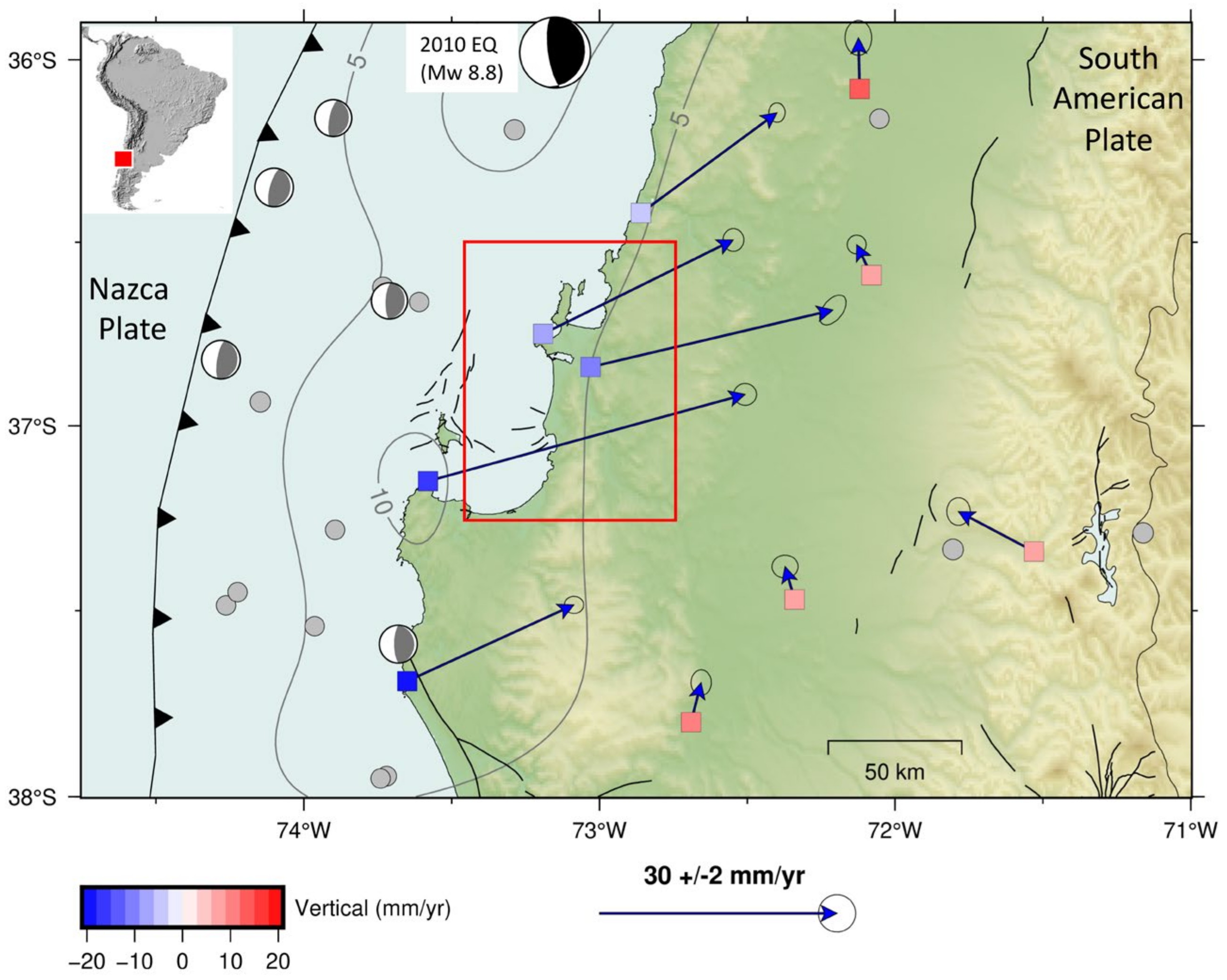
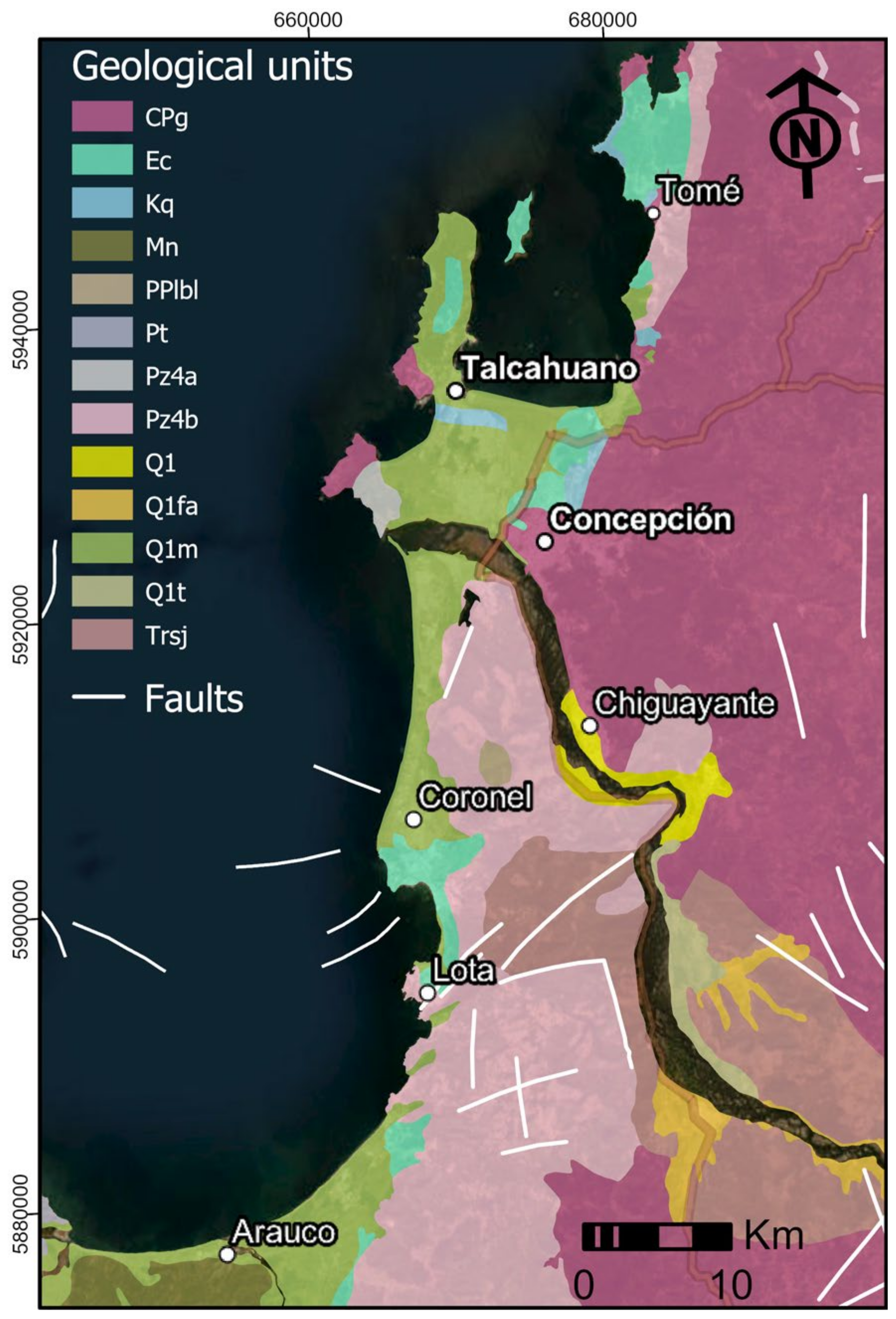
Seismotectonic and Geological Setting
2. InSAR Techniques Methods
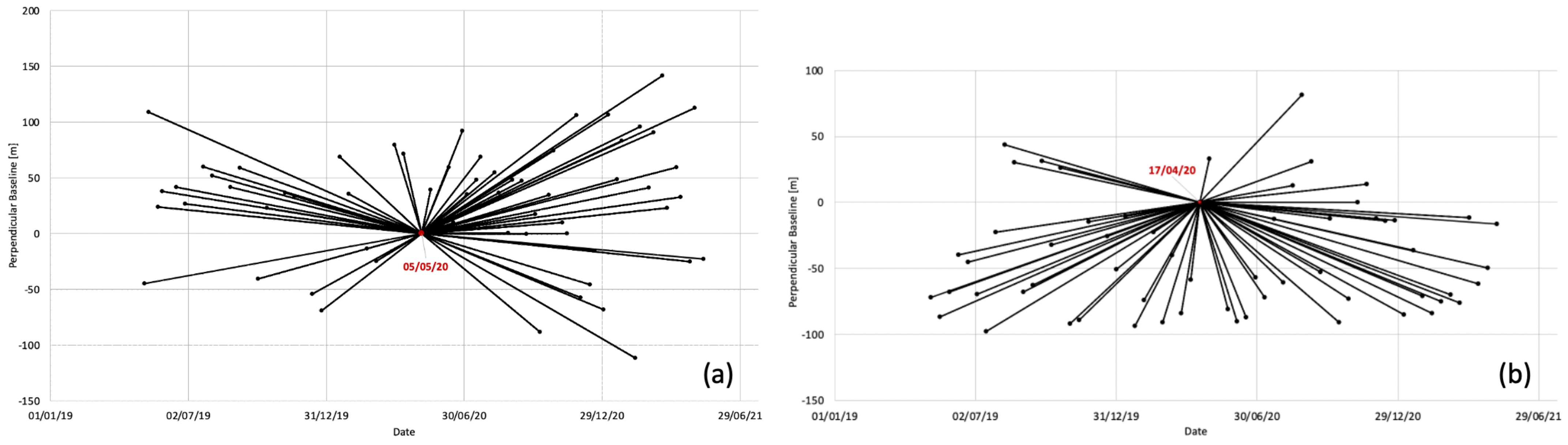
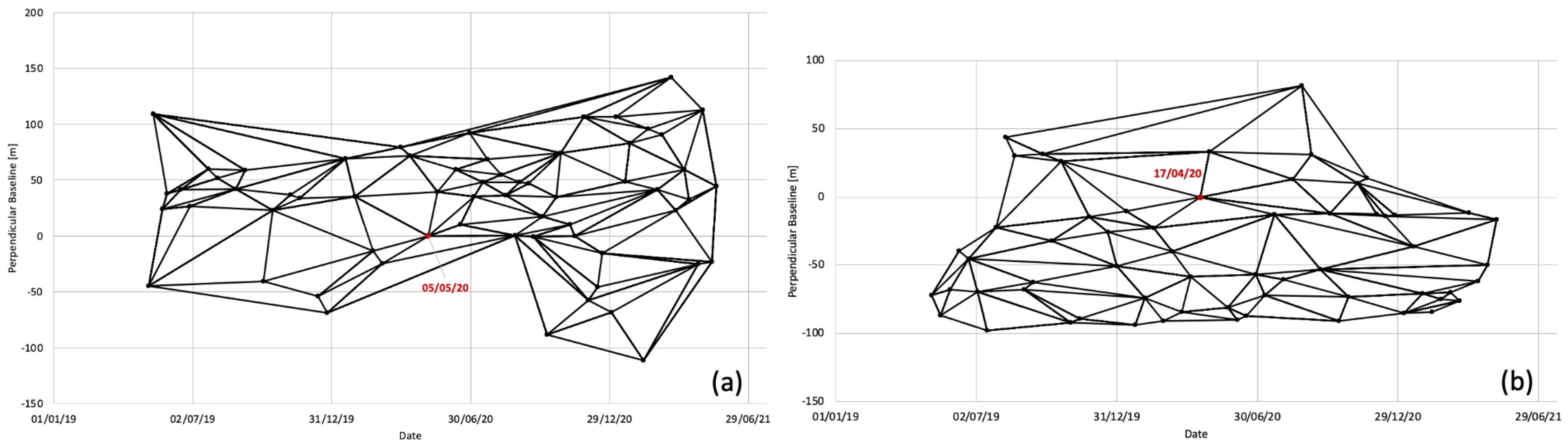
2.1. SAR Data
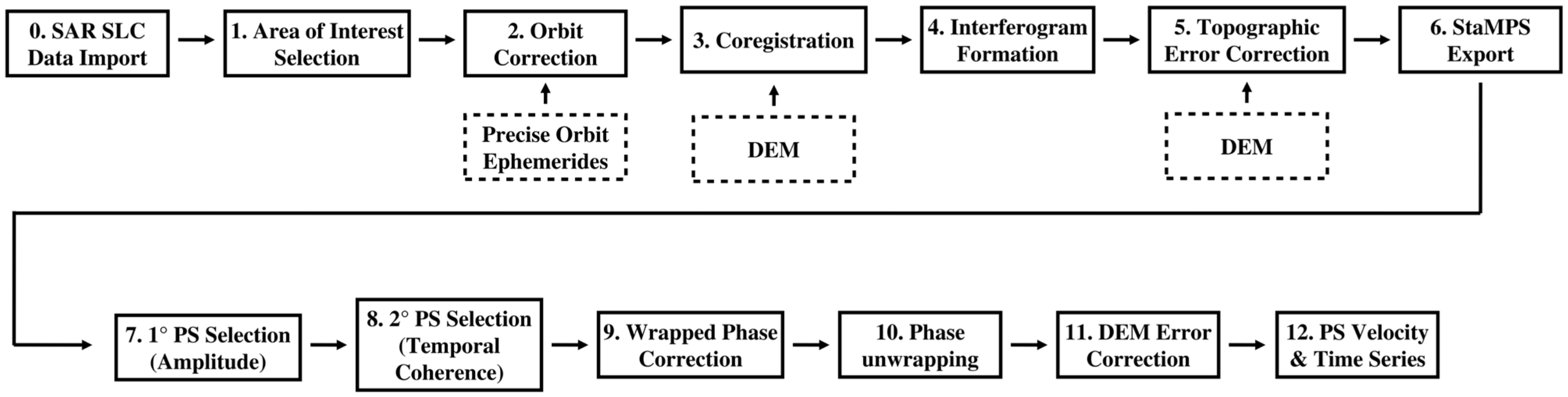
2.2. PSI Techniques
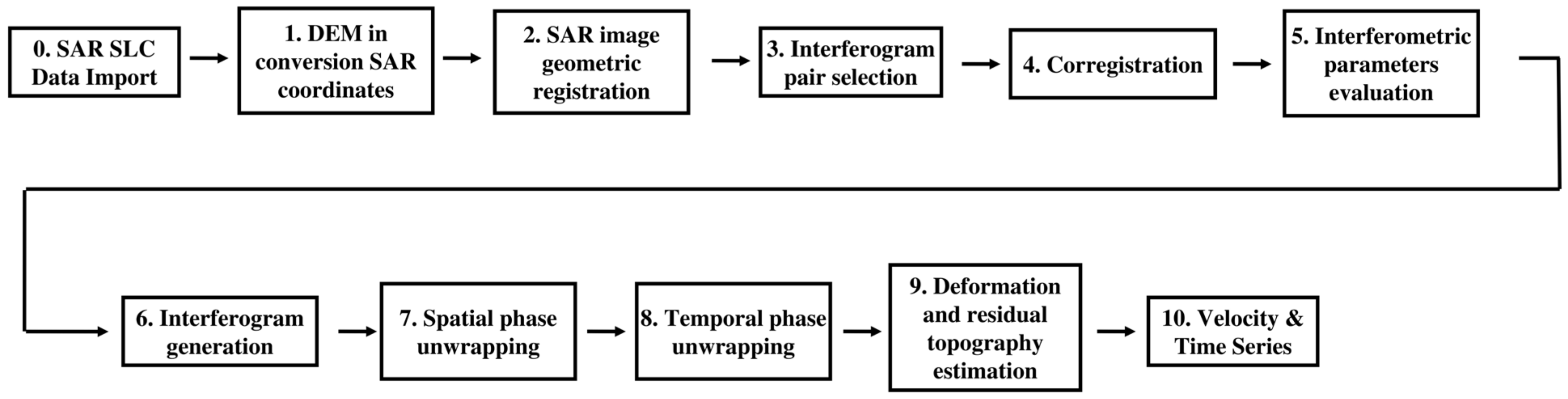
2.3. SBAS Technique
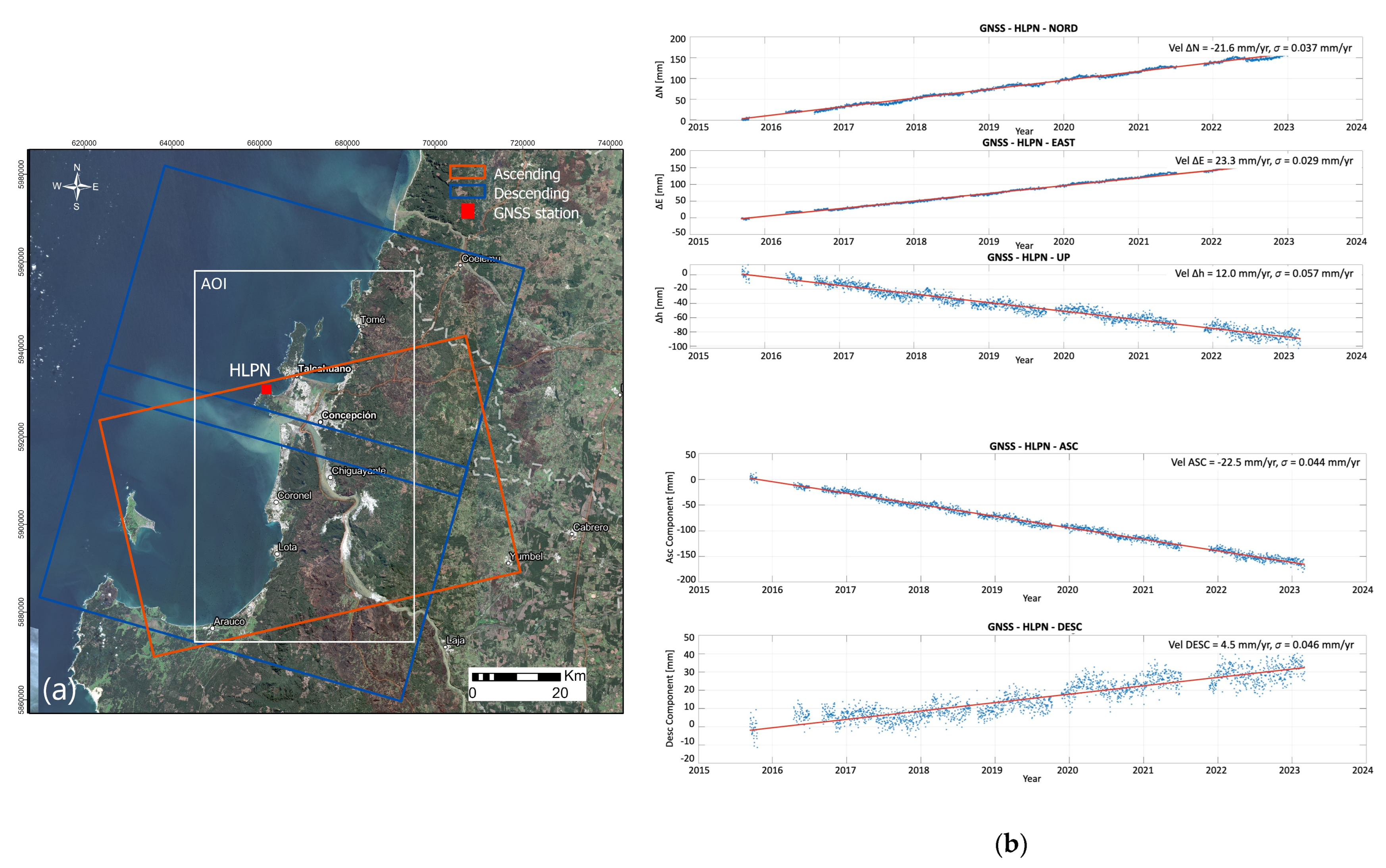
2.4. Post-Processing and Measurements Correction
3. Results and Discussions
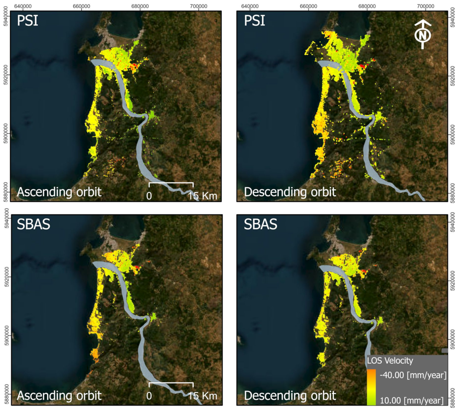
3.1. Ground Deformation Measurements
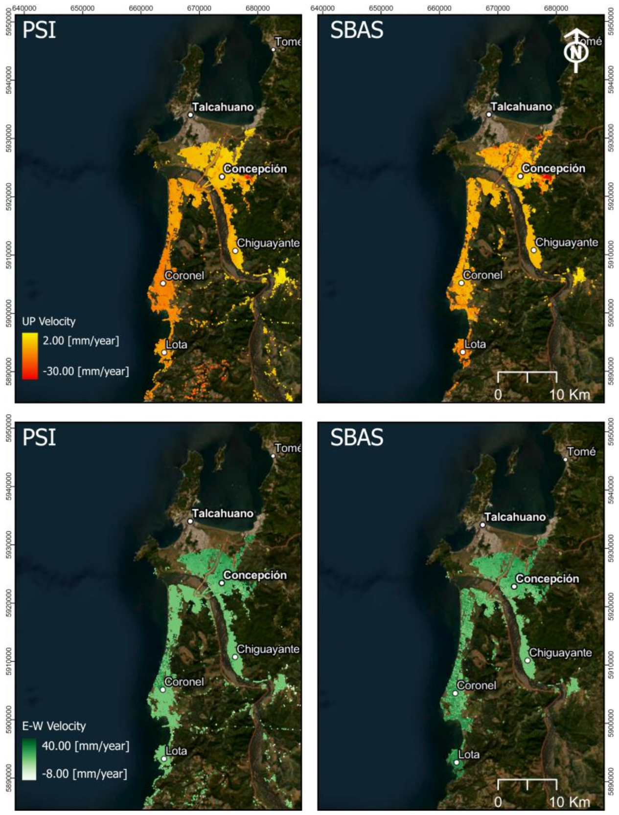
3.2. Vertical and East–West Displacements Analysis
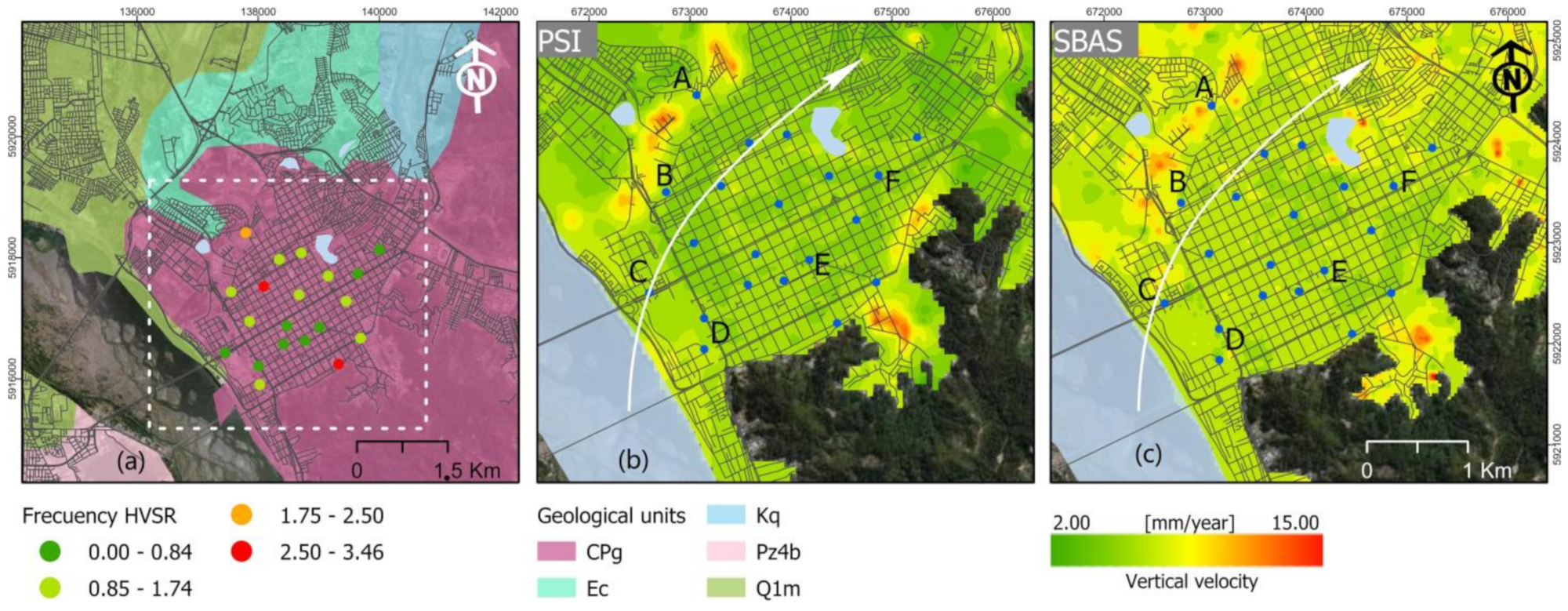
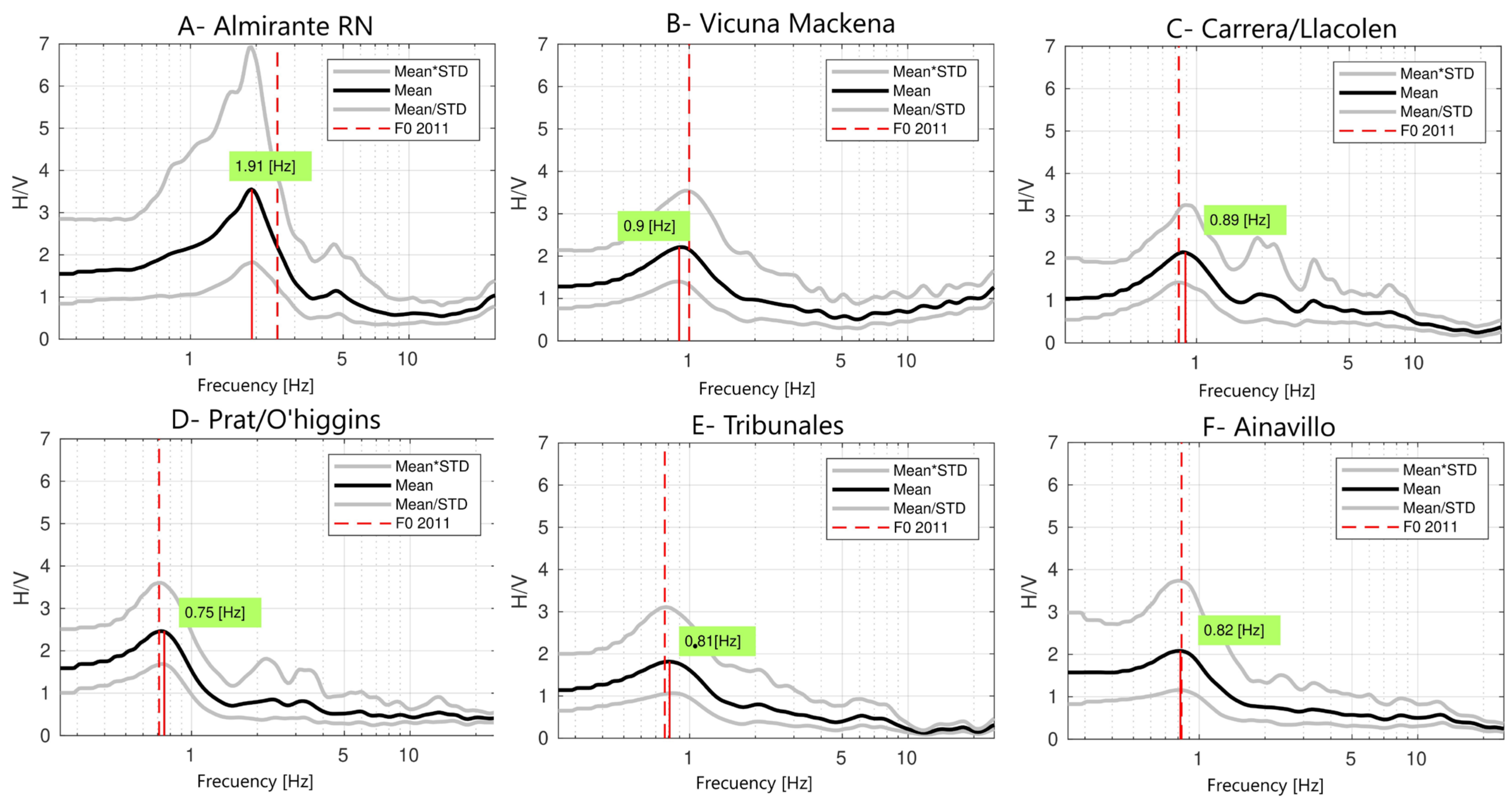
3.3. InSAR Deformation and Site Conditions
4. Conclusions
Author Contributions
Funding
Data Availability Statement
Acknowledgments
Conflicts of Interest
References
- Assimaki, D.; Ledezma, C.; Montalva, G.A.; Tassara, A.; Mylonakis, G.; Boroschek, R. Site effects and damage patterns. Earthq. Spectra 2012, 28 (Suppl. 1), 55–74. [Google Scholar] [CrossRef]
- Bray, J.; Rollins, K.; Hutchinson, T.; Verdugo, R.; Ledezma, C.; Mylonakis, G.; Assimaki, D.; Montalva, G.; Arduino, P.; Olson, S.M.; et al. Effects of ground failure on buildings, ports, and industrial facilities. Earthq. Spectra 2012, 28 (Suppl. 1), 97–118. [Google Scholar] [CrossRef]
- Leyton, F.; Montalva, G.; Ramírez, P. Effects of surface geology on seismic motion. In Proceedings of the 4th IASPEI/IAEEE International Symposium, Santa Barbara, CA, USA, 23–26 August 2011; pp. 1–10. [Google Scholar]
- Berardino, P.; Fornaro, G.; Lanari, R.; Sansosti, E. A new algorithm for surface deformation monitoring based on small baseline differential SAR interferograms. IEEE Trans. Geosci. Remote Sens. 2002, 40, 2375–2383. [Google Scholar] [CrossRef]
- Ferretti, A.; Prati, C.; Rocca, F. Permanent scatterers in SAR interferometry. IEEE Trans. Geosci. Remote Sens. 2001, 39, 8–20. [Google Scholar] [CrossRef]
- Bonano, M.; Manunta, M.; Pepe, A.; Paglia, L.; Lanari, R. From previous C-band to new X-band SAR systems: Assessment of the DInSAR mapping improvement for deformation time-series retrieval in urban areas. IEEE Trans. Geosci. Remote Sens. 2013, 51, 1973–1984. [Google Scholar] [CrossRef]
- Casu, F.; Manzo, M.; Lanari, R. A quantitative assessment of the SBAS algorithm performance for surface deformation retrieval from DInSAR data. Remote Sens. Environ. 2006, 102, 195–210. [Google Scholar] [CrossRef]
- Li, Z.; Wen, Y.; Zhang, P.; Liu, Y.; Zhang, Y. Joint investment of GPS, leveling, and InSAR data for the 2013 Lushan (China) earthquake and its seismic hazard implications. Remote Sens. 2020, 12, 715. [Google Scholar] [CrossRef]
- Weston, J.; Ferreira, A.M.; Funning, G.J. Systematic comparisons of earthquake source models determined using InSAR and seismic data. Tectonophysics 2012, 532, 61–81. [Google Scholar] [CrossRef]
- Orellana, F.; Hormazábal, J.; Montalva, G.; Moreno, M. Measuring Coastal Subsidence after Recent Earthquakes in Central Chile Using SAR Interferometry and GNSS Data. Remote Sens. 2022, 14, 1611. [Google Scholar] [CrossRef]
- Van Natijne, A.L.; Bogaard, T.A.; van Leijen, F.J.; Hanssen, R.F.; Lindenbergh, R.C. World-wide InSAR sensitivity index for landslide deformation tracking. Int. J. Appl. Earth Obs. Geoinf. 2022, 111, 102829. [Google Scholar] [CrossRef]
- Fobert, M.A.; Singhroy, V.; Spray, J.G. InSAR monitoring of landslide activity in Dominica. Remote Sens. 2021, 13, 815. [Google Scholar] [CrossRef]
- Orellana, F.; Moreno, M.; Yáñez, G. High-Resolution Deformation Monitoring from DInSAR: Implications for Geohazards and Ground Stability in the Metropolitan Area of Santiago, Chile. Remote Sens. 2022, 14, 6115. [Google Scholar] [CrossRef]
- Bonì, R.; Herrera, G.; Meisina, C.; Notti, D.; Béjar-Pizarro, M.; Zucca, F.; Gonzalez, P.J.; Palano, M.; Tomás, R.; Fernandez, J.; et al. Twenty-year advanced DInSAR analysis of severe land subsidence: The Alto Guadalentín Basin (Spain) case study. Eng. Geol. 2015, 198, 40–52. [Google Scholar] [CrossRef]
- Ezquerro, P.; Tomás, R.; Béjar-Pizarro, M.; Fernández-Merodo, J.A.; Guardiola-Albert, C.; Staller, A.; Sánchez-Sobrino, J.A.; Herrera, G. Improving multi-technique monitoring using Sentinel-1 and Cosmo-SkyMed data and upgrading groundwater model capabilities. Sci. Total Environ. 2020, 703, 134757. [Google Scholar] [CrossRef] [PubMed]
- Orellana, F.; Rivera, D.; Montalva, G.; Arumi, J.L. InSAR-Based Early Warning Monitoring Framework to Assess Aquifer Deterioration. Remote Sens. 2023, 15, 1786. [Google Scholar] [CrossRef]
- Chang, L.; Dollevoet, R.P.; Hanssen, R.F. Monitoring line-infrastructure with multisensor SAR interferometry: Products and performance assessment metrics. IEEE J. Sel. Top. Appl. Earth Obs. Remote Sens. 2018, 11, 1593–1605. [Google Scholar] [CrossRef]
- De Corso, T.; Mignone, L.; Sebastianelli, A.; del Rosso, M.; Yost, C.; Ciampa, E.; Pecce, M.; Sica, S.; Ullo, S. Application of DInSAR technique to high coherence satellite images for strategic infrastructure monitoring. In Proceedings of the IGARSS 2020–2020 IEEE International Geoscience and Remote Sensing Symposium, Waikoloa, HI, USA, 26 September–2 October 2020; IEEE: New York, NY, USA, 2020; pp. 4235–4238. [Google Scholar]
- Orellana, F.; Delgado Blasco, J.M.; Foumelis, M.; D’Aranno, P.J.; Marseille, M.A.; Di Mascio, P. Dinsar for road infrastructure monitoring: Case study highway network of Rome metropolitan (Italy). Remote Sens. 2020, 12, 3697. [Google Scholar] [CrossRef]
- Orellana, F.; D’Aranno, P.J.; Scifoni, S.; Marsella, M. SAR Interferometry Data Exploitation for Infrastructure Monitoring Using GIS Application. Infrastructures 2023, 8, 94. [Google Scholar] [CrossRef]
- Ho Tong Minh, D.; Hanssen, R.; Rocca, F. Radar interferometry: 20 years of development in time series techniques and future perspectives. Remote Sens. 2020, 12, 1364. [Google Scholar] [CrossRef]
- Ferretti, A.; Prati, C.; Rocca, F. Nonlinear subsidence rate estimation using permanent scatterers in differential SAR interferometry. IEEE Trans. Geosci. Remote Sens. 2000, 38, 2202–2212. [Google Scholar] [CrossRef]
- Hooper, A.; Zebker, H.; Segall, P.; Kampes, B. A new method for measuring deformation on volcanoes and other natural terrains using InSAR persistent scatterers. Geophys. Res. Lett. 2004, 31. [Google Scholar] [CrossRef]
- Van der Kooij, M.; Lacoste, H. Coherent target analysis. In Proceedings of the Third International Workshop on ERS SAR Interferometry (FRINGE 2003), Frascati, Italy, 20 August 2003; pp. 2–5. [Google Scholar]
- Kampes, B.M. Radar Interferometry; Springer: Dordrecht, The Netherlands, 2006; Volume 12. [Google Scholar]
- Costantini, M.; Falco, S.; Malvarosa, F.; Minati, F. A new method for identification and analysis of persistent scatterers in series of SAR images. In Proceedings of the IGARSS 2008–2008 IEEE International Geoscience and Remote Sensing Symposium, Boston, MA, USA, 6–11 July 2008; IEEE: New York, NY, USA; Volume 2, pp. II-449–II-452. [Google Scholar]
- Perissin, D.; Wang, T. Repeat-pass SAR interferometry with partially coherent targets. IEEE Trans. Geosci. Remote Sens. 2011, 50, 271–280. [Google Scholar] [CrossRef]
- Devanthéry, N.; Crosetto, M.; Monserrat, O.; Cuevas-González, M.; Crippa, B. An approach to persistent scatterer interferometry. Remote Sens. 2014, 6, 6662–6679. [Google Scholar] [CrossRef]
- Lanari, R.; Mora, O.; Manunta, M.; Mallorquí, J.J.; Berardino, P.; Sansosti, E. A small-baseline approach for investigating deformations on full-resolution differential SAR interferograms. IEEE Trans. Geosci. Remote Sens. 2004, 42, 1377–1386. [Google Scholar] [CrossRef]
- Hong, S.H.; Wdowinski, S.; Kim, S.W.; Won, J.S. Multi-temporal monitoring of wetland water levels in the Florida Everglades using interferometric synthetic aperture radar (InSAR). Remote Sens. Environ. 2010, 114, 2436–2447. [Google Scholar] [CrossRef]
- Hetland, E.A.; Musé, P.; Simons, M.; Lin, Y.N.; Agram, P.S.; DiCaprio, C.J. Multiscale InSAR time series (MINTS) analysis of surface deformation. J. Geophys. Res. Solid Earth 2012, 117. [Google Scholar] [CrossRef]
- Yunjun, Z.; Fattahi, H.; Amelung, F. Small baseline InSAR time series analysis: Unwrapping error correction and noise reduction. Comput. Geosci. 2019, 133, 104331. [Google Scholar] [CrossRef]
- Casu, F.; Elefante, S.; Imperatore, P.; Zinno, I.; Manunta, M.; De Luca, C.; Lanari, R. SBAS-DInSAR parallel processing for deformation time-series computation. IEEE J. Sel. Top. Appl. Earth Obs. Remote Sens. 2014, 7, 3285–3296. [Google Scholar] [CrossRef]
- Manunta, M.; De Luca, C.; Zinno, I.; Casu, F.; Manzo, M.; Bonano, M.; Fusco, A.; Pepe, A.; Onorato, G.; Berardino, P.; et al. The parallel SBAS approach for Sentinel-1 interferometric wide swath deformation time-series generation: Algorithm description and products quality assessment. IEEE Trans. Geosci. Remote Sens. 2019, 57, 6259–6281. [Google Scholar] [CrossRef]
- Torres, R.; Snoeij, P.; Geudtner, D.; Bibby, D.; Davidson, M.; Attema, E.; Potin, P.; Rommen, B.; Floury, N.; Brown, M.; et al. GMES Sentinel-1 mission. Remote Sens. Environ. 2012, 120, 9–24. [Google Scholar] [CrossRef]
- De Zan, F.; Guarnieri, A.M. TOPSAR: Terrain observation by progressive scans. IEEE Trans. Geosci. Remote Sens. 2006, 44, 2352–2360. [Google Scholar] [CrossRef]
- Cigna, F.; Esquivel Ramírez, R.; Tapete, D. Accuracy of Sentinel-1 PSI and SBAS InSAR Displacement Velocities against GNSS and Geodetic Leveling Monitoring Data. Remote Sens. 2021, 13, 4800. [Google Scholar] [CrossRef]
- Adam, N.; Parizzi, A.; Eineder, M.; Crosetto, M. Practical persistent scatterer processing validation in the course of the Terrafirma project. J. Appl. Geophys. 2009, 69, 59–65. [Google Scholar] [CrossRef]
- Cigna, F.; Sowter, A. The relationship between intermittent coherence and precision of ISBAS InSAR ground motion velocities: ERS-1/2 case studies in the UK. Remote Sens. Environ. 2017, 202, 177–198. [Google Scholar] [CrossRef]
- Pepe, A. Multi-temporal small baseline interferometric SAR algorithms: Error budget and theoretical performance. Remote Sens. 2021, 13, 557. [Google Scholar] [CrossRef]
- Moreno, M.; Melnick, D.; Rosenau, M.; Baez, J.; Klotz, J.; Oncken, O.; Tassara, A.; Chen, J.; Bataille, K.; Bevis, M.; et al. Toward understanding tectonic control on the Mw 8.8 2010 Maule Chile earthquake. Earth Planet. Sci. Lett. 2012, 321, 152–165. [Google Scholar] [CrossRef]
- Yáñez-Cuadra, V.; Moreno, M.; Ortega-Culaciati, F.; Donoso, F.; Báez, J.C.; Tassara, A. Mosaicking Andean morphostructure and seismic cycle crustal deformation patterns using GNSS velocities and machine learning. Front. Earth Sci. 2023, 11, 1096238. [Google Scholar] [CrossRef]
- SERNAGEOMN—National Geology and Mining Service, Source Open Geological Map of Chile. Available online: https://www.sernageomin.cl/geologia/ (accessed on 15 May 2023).
- Montalva, G.A.; Chávez-Garcia, F.J.; Tassara, A.; Jara Weisser, D.M. Site effects and building damage characterization in Concepción after the Mw 8.8 Maule earthquake. Earthq. Spectra 2016, 32, 1469–1488. [Google Scholar] [CrossRef]
- Galli, C. Geología urbana y suelos de fundación de Concepción y Talcahuano. In Informe Final del Proyecto de Investigación N°75 de la Comisión de Investigación Científica de la Universidad de Concepción; Universidad de Concepción: Concepción, Chile, 1967. (In Spanish) [Google Scholar]
- Vivallos, J.; Ramírez, P.Y.; Fonseca, A. Microzonificación Sísmica de la Ciudad de Concepción, Región del Biobío. Servicio Nacional de Geología y Minería. Carta Geológica de Chile, Serie Geológica Ambiental X. 3 Mapa Escala 1:20.000; Servicio Nacional de Geología y Minería: Santiago, Chile, 2009. [Google Scholar]
- Xu, B.; Li, Z.; Zhu, Y.; Shi, J.; Feng, G. Kinematic coregistration of sentinel-1 TOPSAR images based on sequential least squares adjustment. IEEE J. Sel. Top. Appl. Earth Obs. Remote Sens. 2020, 13, 3083–3093. [Google Scholar] [CrossRef]
- Foumelis, M.; Blasco, J.M.D.; Desnos, Y.L.; Engdahl, M.; Fernández, D.; Veci, L.; Lu, J.; Wong, C. ESA SNAP-StaMPS integrated processing for Sentinel-1 persistent scatterer interferometry. In Proceedings of the IGARSS 2018–2018 IEEE International Geoscience and Remote Sensing Symposium, Valencia, Spain, 22–27 July 2018; IEEE: New York, NY, USA, 2018; pp. 1364–1367. [Google Scholar]
- Hooper, A.; Spaans, K.; Bekaert, D.; Cuenca, M.C.; Arıkan, M.; Oyen, A. StaMPS/MTI Manual; Delft Institute of Earth Observation and Space Systems Delft University of Technology: Delft, The Netherlands, 2010; Volume 1, p. 2629. [Google Scholar]
- Hooper, A.; Segall, P.; Zebker, H. Persistent Scatterer Interferometric Synthetic Aperture Radar for Crustal Deformation Analysis, with applications to Volcàn Alcedo. J. Geophys. Res. 2007, 112. [Google Scholar] [CrossRef]
- Delgado Blasco, J.M.; Foumelis, M.; Stewart, C.; Hooper, A. Measuring urban subsidence in the Rome metropolitan area (Italy) with Sentinel-1 SNAP-StaMPS persistent scatterer interferometry. Remote Sens. 2019, 11, 129. [Google Scholar] [CrossRef]
- Lanari, R.; Casu, F.; Manzo, M.; Zeni, G.; Berardino, P.; Manunta, M.; Pepe, A. An overview of the small baseline subset algorithm: A DInSAR technique for surface deformation analysis. In Deformation and Gravity Change: Indicators of Isostasy Tectonics, Volcanism, and Climate Change; Birkhäuser: Basel, Switzerland, 2007; pp. 637–661. [Google Scholar]
- Zebker, H.A.; Villasenor, J. Decorrelation in interferometric radar echoes. IEEE Trans. Geosci. Remote Sens. 1992, 30, 950–959. [Google Scholar] [CrossRef]
- De Luca, C.; Bonano, M.; Casu, F.; Fusco, A.; Lanari, R.; Manunta, M.; Pepe, A.; Zinno, I. Automatic and systematic Sentinel-1 SBAS-DInSAR processing chain for deformation time-series generation. Procedia Comput. Sci. 2016, 100, 1176–1180. [Google Scholar] [CrossRef]
- Zinno, I.; Casu, F.; De Luca, C.; Elefante, S.; Lanari, R.; Manunta, M. A cloud computing solution for the efficient implementation of the P-SBAS DInSAR approach. IEEE J. Sel. Top. Appl. Earth Obs. Remote Sens. 2016, 10, 802–817. [Google Scholar] [CrossRef]
- Imperatore, P.; Pepe, A.; Sansosti, E. High performance computing in satellite SAR interferometry: A critical perspective. Remote Sens. 2021, 13, 4756. [Google Scholar] [CrossRef]
- De Luca, C.; Cuccu, R.; Elefante, S.; Zinno, I.; Manunta, M.; Casola, V.; Rivolta, G.; Lanari, R.; Casu, F. An On-Demand Web Tool for the Unsupervised Retrieval of Earth’s Surface Deformation from SAR Data: The P-SBAS Service within the ESA G-POD Environment. Remote Sens. 2015, 7, 15630–15650. [Google Scholar] [CrossRef]
- SONEL Serves as the GNSS Data Assembly Centre for the Global Sea Level Observing System (GLOSS); p. 61. Available online: https://www.sonel.org/spip.php?page=gps&idStation=4491 (accessed on 1 June 2023).
- The International Terrestrial Reference Frame (ITRF). Available online: https://www.iers.org/IERS/EN/DataProducts/ITRF/itrf.html (accessed on 1 June 2023).
- Catalão, J.; Nico, G.; Hanssen, R.; Catita, C. Integration of InSAR and GPS for vertical deformation monitoring: A case of study in Faial and Pico Islands. In Proceedings of the Fringe 2009 Workshop, Frascati, Italy, 30 November–4 December 2009. [Google Scholar]
- Samsonov, S.; Tiampo, K. Analytical optimization of a DInSAR and GPS dataset for derivation of three-dimensional surface motion. IEEE Geosci. Remote Sens. Lett. 2006, 3, 107–111. [Google Scholar] [CrossRef]
- Fuhrmann, T.; Garthwaite, M.C. Resolving three-dimensional surface motion with InSAR: Constraints from multi-geometry data fusion. Remote Sens. 2019, 11, 241. [Google Scholar] [CrossRef]
- Cigna, F.; Tapete, D. Sentinel-1 big data processing with P-SBAS InSAR in the geohazards exploitation platform: An experiment on coastal land subsidence and landslides in Italy. Remote Sens. 2021, 13, 885. [Google Scholar] [CrossRef]
- Link, O.; Brox-Escudero, L.M.; González, J.; Aguayo, M.; Torrejón, F.; Montalva, G.; Eguibar-Galán, M.Á. A paleo-hydro-geomorphological perspective on urban flood risk assessment. Hydrol. Process. 2019, 33, 3169–3183. [Google Scholar] [CrossRef]
- Leyton, F.; Sepúlveda, S.A.; Astroza, M.; Rebolledo, S.; Acevedo, P.; Ruiz, S.; Gonzalez, L.; Foncea, C. Seismic zonation of the Santiago Basin, Chile. In Proceedings of the Fifth International Conference on Earthquake Geotechnical Engineering 2011, Santiago, Chile, 10–13 January 2011. [Google Scholar]
- Montalva, G.A.; Bastías, N.; Leyton, F. Strong ground motion prediction model for PGV and spectral velocity for the Chilean subduction zone. Bull. Seismol. Soc. Am. 2022, 112, 348–360. [Google Scholar] [CrossRef]


| Orbit | Ascending | Descending |
|---|---|---|
| Sensor | Sentinel-1A–1B | Sentinel-1A–1B |
| N° acquisition | 60 | 60 |
| Start date | 05/05/2019 | 05/05/2019 |
| End date | 05/05/2021 | 05/05/2021 |
| Orbit | 86 | 156 |
| Polarization | VV | VV |
| Swath | IW2 | IW2–IW3 |
| Bursts | 4–6 | 5–7 |
| Technique (Range × Azimuth) | UP Velocity (mm/year) (min|mean|max) | East Velocity (mm/year) (min|max) |
|---|---|---|
| SBAS (90 × 90 mt) | −27.69|−12.31|−3.82 | 8.10|23.01|38.70 |
| PSI (20 × 20 mt) | −25.12|−12.27|−5.60 | 9.30|23.56|35.11 |
| Points—Locations | F0_2011 | F0_2023 | Anomaly |
|---|---|---|---|
| A—Almirante RN | 2.50 | 1.91 | −0.59 |
| B—Vicuna Mackena | 1.00 | 0.90 | −0.10 |
| C—Carrera/Llacolen | 0.83 | 0.89 | 0.06 |
| D—Prat/O’higgins | 0.71 | 0.75 | 0.04 |
| E—Tribunales | 0.77 | 0.81 | 0.04 |
| F—Ainavillo | 0.83 | 0.82 | −0.01 |
Disclaimer/Publisher’s Note: The statements, opinions and data contained in all publications are solely those of the individual author(s) and contributor(s) and not of MDPI and/or the editor(s). MDPI and/or the editor(s) disclaim responsibility for any injury to people or property resulting from any ideas, methods, instructions or products referred to in the content. |
© 2023 by the authors. Licensee MDPI, Basel, Switzerland. This article is an open access article distributed under the terms and conditions of the Creative Commons Attribution (CC BY) license (https://creativecommons.org/licenses/by/4.0/).
Share and Cite
Giorgini, E.; Orellana, F.; Arratia, C.; Tavasci, L.; Montalva, G.; Moreno, M.; Gandolfi, S. InSAR Monitoring Using Persistent Scatterer Interferometry (PSI) and Small Baseline Subset (SBAS) Techniques for Ground Deformation Measurement in Metropolitan Area of Concepción, Chile. Remote Sens. 2023, 15, 5700. https://doi.org/10.3390/rs15245700
Giorgini E, Orellana F, Arratia C, Tavasci L, Montalva G, Moreno M, Gandolfi S. InSAR Monitoring Using Persistent Scatterer Interferometry (PSI) and Small Baseline Subset (SBAS) Techniques for Ground Deformation Measurement in Metropolitan Area of Concepción, Chile. Remote Sensing. 2023; 15(24):5700. https://doi.org/10.3390/rs15245700
Chicago/Turabian StyleGiorgini, Eugenia, Felipe Orellana, Camila Arratia, Luca Tavasci, Gonzalo Montalva, Marcos Moreno, and Stefano Gandolfi. 2023. "InSAR Monitoring Using Persistent Scatterer Interferometry (PSI) and Small Baseline Subset (SBAS) Techniques for Ground Deformation Measurement in Metropolitan Area of Concepción, Chile" Remote Sensing 15, no. 24: 5700. https://doi.org/10.3390/rs15245700
APA StyleGiorgini, E., Orellana, F., Arratia, C., Tavasci, L., Montalva, G., Moreno, M., & Gandolfi, S. (2023). InSAR Monitoring Using Persistent Scatterer Interferometry (PSI) and Small Baseline Subset (SBAS) Techniques for Ground Deformation Measurement in Metropolitan Area of Concepción, Chile. Remote Sensing, 15(24), 5700. https://doi.org/10.3390/rs15245700