Abstract
Hyperspectral anomaly detection (HAD) is of great interest for unknown exploration. Existing methods only focus on local similarity, which may show limitations in detection performance. To cope with this problem, we propose a relationship attention-guided unsupervised learning with convolutional autoencoders (CAEs) for HAD, called RANet. First, instead of only focusing on the local similarity, RANet, for the first time, pays attention to topological similarity by leveraging the graph attention network (GAT) to capture deep topological relationships embedded in a customized incidence matrix from absolutely unlabeled data mixed with anomalies. Notably, the attention intensity of GAT is self-adaptively controlled by adjacency reconstruction ability, which can effectively reduce human intervention. Next, we adopt an unsupervised CAE to jointly learn with the topological relationship attention to achieve satisfactory model performance. Finally, on the basis of background reconstruction, we detect anomalies by the reconstruction error. Extensive experiments on hyperspectral images (HSIs) demonstrate that our proposed RANet outperforms existing fully unsupervised methods.
1. Introduction
As an image type that can capture spectral intrinsic information with the help of advanced imaging technology, hyperspectral images (HSIs) are usually represented in three dimensions; the first two dimensions show spatial information, and the third dimension records spectral information, which is used to reflect different properties of different substances [1,2,3,4,5,6]. Compared to ordinary RGB images, HSIs have more spectral bands, which can store richer information and depict more details of the captured scenes. Currently, HSIs have been widely used in the fields of resource exploration, environmental monitoring, precision agriculture and management [7,8,9,10,11]. On this basis, various data analysis methods such as classification, target detection and anomaly detection have emerged. Among them, hyperspectral anomaly detection (HAD), which performs unsupervised detection of objects that are spatially or spectrally different from the surrounding background, has received increasing attention in practical applications [12,13,14,15,16]. However, due to some real-world resource constraints such as lack of prior knowledge, low spatial resolution [17], lack of labels and insufficient sample sets bring many difficulties to HAD.
Existing methods are mainly divided into two categories: traditional methods and deep neural network (DNN)-based methods. Assuming that the background obeys multivariate Gaussian normal distribution, the Reed Xiaoli (RX) algorithm [18], by Reed and Yu, has been proposed. If an RX detector estimates the background model using local statistics, this is an improved variant called local RX (LRX) [19]. Other traditional algorithms such as CRD [20], SRD [21], LSMAD [22] and LRASR [23] construct models by characterizing local neighbor pixels. These traditional methods have limited ability to characterize high-dimensional and complex data, thus making it difficult to achieve performance improvements. Under this circumstance, several efforts dedicated to determining hyperspectral anomalies by DNNs without any prior knowledge have been developed. DNN-based methods relying on AE [17] and GAN [24] focus on minimizing the error of each spectral vector in the original image and reconstructed image. Other DNN-based methods like CNN [25] take local similarity of spectra into consideration. Typically, these methods either interest a single spectral vector or consider local spectral similarity. However, they usually suffer from ignoring the topological relationship in HSIs. For instance, as shown in Figure 1, some anomalies are spectrally similar, whereas they are far apart in spatial dimensions, which makes most algorithms falsely consider anomalies as background. In addition, the blind introduction of hand-craft topological relationships may also degrade the model capability and generalizability in handling diverse HSIs.

Figure 1.
An illustration of the existing methods. Some anomalies (red blocks) are far apart in spatial dimensions and, thus, may be considered as background (blue blocks).
To address the aforementioned limitations, based on the observation that some anomalies are very far apart in the spatial domain, we put forward a relationship attention network for HAD, named RANet. Instead of hand-craft prior, RANet adopts an attention module that learns deep topological relationships from original HSIs in an end-to-end manner, where the attention intensity is self-adaptively controlled by adjacency reconstruction ability, which can effectively reduce human intervention. In this way, different categories have different topological relationships, which can better adapt to the characteristics of HSIs to achieve end-to-end personalized model learning. Furthermore, to address the difficulty in defining the neighbor relationship of an anomaly in a high-dimensional space, we leverage a graph attention network (GAT) with a customized incidence matrix to drive the non-local topological relationship between anomalies more significant without the need to know the structure of the whole HSIs. In particular, the customized incidence matrix, which utilizes spectral angle distance (SAD) instead of Euclidean distance (ED) to calculate the distance between spectral vectors, is imposed to better capture spectral similarity. More importantly, to make full use of correlations among adjacency, we establish an unsupervised CAE to determine anomalies, which is jointly learned with the topological relationship attention to achieve promising model accuracy.
The main contributions of our work are as follows:
- We propose a novel framework, RANet, for hyperspectral anomaly detection. To the best of our knowledge, this is the first attempt to explore the potential of topological relationships in this task;
- We introduce a customized incidence matrix that directs GAT to pay attention to topological relationships in HSIs, where the attention intensity is self-adaptively adjusted to different data characteristics;
- Furthermore, an end-to-end unsupervised CAE with high-fidelity and high-dimensional data representation is developed as the reconstruction backbone;
- We jointly learn the reconstructed backbone and topological attention to detect anomalies with the reconstruction error. Extensive experiments on HSIs indicate that our RANet outperforms existing state-of-the-art methods.
2. Related Work
Deep neural networks (DNNs) have attracted much attention in the field of HAD because they can estimate complex functions through hierarchical structures and capture hidden features; thus, DNN-based anomaly detection technologies have been applied to many fields [26,27,28,29]. Among them, unsupervised learning models have become mainstream research topics because they do not require label information. Autoencoders (AEs) can achieve automatic selection of features and improve the interpretability of networks. To tackle the problems of high dimensionality, redundant information and degenerate bands of hyperspectral images, a spectral constraint AAE (SC_AAE) [30] incorporates a spectral constraint strategy into adversarial autoencoders (AAE) to perform HAD. It introduces the spectral angular distance in the loss function to enhance spectral consistency. Liu et al. [31] introduced a dual-frequency autoencoder (DFAE) detection model to enhance the separability of background anomalies while breaking the dilemma of limited generalization ability in no-sample HAD tasks. An unsupervised low-rank embedded network (LREN) [6] estimates residuals efficiently in deep latent spaces by searching the lowest-rank representation based on a representative and discriminative dictionary. Additionally, Xie et al. [32] constructed a spectral distribution-aware estimation network (SDEN) that does not conduct feature extraction and anomaly detection in two separate steps but instead learns both jointly to estimate anomalies. However, since AEs perform feature learning for each spectral vector, the similarity between local spectral vectors is not considered. Convolutional autoencoders (CAEs) pay attention to local similarity by combining the convolution and pooling operations of the convolutional neural network and realize a deep neural network through stacking. Considering that the structure of the convolutional image generator for hyperspectral images can capture a large number of image statistics, Auto-AD [33] designs a network to reconstruct the background through a fully convolutional AE skip connection. The main advantage of generative adversarial network (GAN) is that it surpasses the functions of traditional neural network classification and feature extraction and can generate new data according to the characteristics of real data. Jiang et al. [34] introduced a weakly supervised discriminant learning algorithm based on spectrally constrained GAN, which utilizes background homogenization and anomaly saliency to enhance the ability to identify anomalies and backgrounds when the anomaly samples are limited and sensitive to the background. Based on the assumption that the number of normal samples is much larger than the number of abnormal samples, HADGAN [35] proposed a generative adversarial network for HAD under unsupervised discriminative reconstruction constraints. Fu et al. [36] proposed a new solution using the plug-and-play framework. To be more specific, by implementing a plug-in framework, the denoiser is employed as a prior for the representation coefficients, while a refined dictionary construction method is suggested to acquire a more refined background dictionary. Introducing BSDM (Background Suppression Diffusion Model), Ma et al. [37] proposed a novel solution for HAD that enables the simultaneous learning of latent background distributions and generalization to diverse datasets, facilitating the suppression of complex backgrounds. Wang et al. [38] proposed a tensor low-rank and sparse representation method for HAD. They put forward a strategy for constructing dictionaries that relies on the weighted tensor kernel norm and sparse regularization norm, aiming to separate low-rank backgrounds from outliers. Although the above-mentioned methods seem to achieve good performance, ignoring topological relationships limits the improvement of detection accuracy.
3. Proposed Method
In this section, we propose RANet for HAD. We describe the overall structure of RANet in Section 3.1, followed by the topological-aware module in Section 3.2. Then, the details of reconstructed backbone are given in Section 3.3 and, finally, the joint learning part in Section 3.4.
3.1. Overall Architecture
An HSI dataset with Z spectral bands and pixels in spatial domain is denoted as , where represents the spectral vector of the ith pixel. consists of a background sample set and an anomaly sample set , which have different characteristics in both spectral and spatial domains, i.e., . Since DNN-based models are data-driven and has much more learnable samples than , existing DNN-based unsupervised HAD methods usually focus on learning the representation of each sample , which leads to small reconstruction errors in background samples and large reconstruction errors in anomaly samples. This process essentially constructs a model that indicates the quality of reconstruction, which can be expressed as
where is the reconstructed HSI and represents the parameters of the reconstruction model , which are learned from the intrinsic characteristics of each sample .
However, these methods may not be ideal because they only pay attention to the latent features of each sample and ignore the connections between samples, especially those that are spatially distant. With these in mind, we introduce the topological relationship into the classical reconstruction model , which serves as an attention mechanism to make the model achieve better representation learning. Formally, we define our reconstruction model as
where is learned not only from each sample , but also from the topological relationships that exist between different samples.
Considering that it is a time-consuming task to calculate the topological relationship between each sample and that the spectral vectors within the local region of HSI have high similarity, we divide an HSI with into P small 3D cubes and denote them as . Here, represents the ith cube, consisting of spectral vectors, i.e., . Therefore, our model is modified as
The learning objective of our model is that the reconstructed background samples outperform the abnormal samples, such that the difference between the original and the reconstructed represents anomalies to be detected. Figure 2 shows a high-level overview of the proposed RANet, which is composed of three major components: topological-aware module, reconstructed backbone and joint learning. Next, we introduce how to design and learn our reconstruction model with these three components.
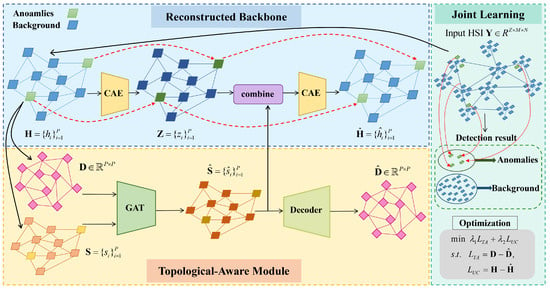
Figure 2.
High-level overview of the proposed RANet. For the topological-aware (TA) module part, we first use an incidence matrix D and a representation set S as input to GAT, to obtain a topological feature map . The reconstruction of D (denoted as ) is gained after the decoding process. As for the reconstructed backbone part, we then use CAE as our network backbone, combined with the previously obtained , to reconstruct H into . The joint learning part is responsible for jointly learning the TA module and the reconstructed backbone in an end-to-end manner.
3.2. Topological-Aware Module
The topological-aware (TA) module intends to dig out deep topological relationships embedded in the customized incidence matrix to guide the reconstruction backbone for high-fidelity background sample representation. In other words, the TA module attempts to acquire the topological relationships of HSI, i.e., , and inject them as attention intensity into the reconstruction model . Given that HAD lacks prior knowledge, we let the TA module learn in an unsupervised manner, which can be subdivided into three parts: customized incidence matrix, topological feature extraction and decoding for reconstruction.
The customized incidence matrix is used to reflect neighbor relationship of HSI’s cube set . Concretely, taking the inherent spectral characteristics of HSI into consideration, we employ the spectral angle distance (SAD) instead of Euclidean distance as the similarity measure to determine the neighbor cubes of each cube. The higher the similarity between two cubes, the more likely they are to be neighbors. The SAD depicts the included angle of two spectral vectors. A smaller SAD value indicates that the spectral vectors are more similar. As shown in Figure 3, two spectral curves from the homogeneous background may have large Euclidean distances even if their shapes are highly similar. On the contrary, their SAD is not affected by the difference in absolute gray values. Therefore, it is reasonable to use SAD to determine the neighbor relationship of in the HAD task. Formally, the incidence matrix can be described as , where represents the similarity between the ith and jth cubes. Thus, the construction of is formulated as
Here, and are reshaped as -dimension vectors before calculation. represents the threshold to determine how close two cubes are to be considered neighbors; its value is discussed in experiments part.
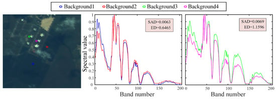
Figure 3.
(Left): Locations of the background samples in the pseudo-color image. (Middle) and (Right): Spectral curves of the background samples in the corresponding color. The legend indicates the spectral angle distance (SAD) and the Euclidean distance (ED) of the two spectral curves.
The topological feature extraction is achieved by a graph attention network (GAT). For easier and more efficient operation, we represent each cube by the average of all spectral vectors in that cube according to local similarity and generate a representation set , where . Thus, the topological features of the entire HSI are obtained by the weighted sum of the representation of each cube and its neighbors
where represents the topological feature, which is combined with the reconstructed backbone later. indicates the neighbor set of the cube representation , which can be retrieved by the customized incidence matrix . means the neighbor of , and is the weight coefficient of this neighbor.
Since different neighbors have different importance, the weight coefficient of each neighbor is acquired using the GAT learning:
Specifically, we first apply a shared linear transformation matrix to standardize the representation vector of each cube. Then, a single-layer neural network parameterized by and is established with the nonlinear activation function LeakyReLU:
where || means the concatenation operation and represents the weight coefficient of to . To normalize the weight coefficient among different cubes, a Softmax function is employed to obtain the final weight coefficient :
The decoding process is designed to learn the parameters and , which is inspired by the autoencoder network. Different from the general autoencoder network, we design a simple and effective decoding method for reconstruction based on data features of the incidence matrix , including dimensional and numerical, without introducing additional learnable parameters. The decoding process is defined as
where × denotes matrix multiplication and refers to the reconstruction of . Consequently, after optimizing the learnable parameters and by minimizing the reconstruction error , the topological feature is ready for the reconstruction backbone.
3.3. Reconstructed Backbone
The backbone of our reconstruction model is configured with an autoencoder. Compared with a fully connected autoencoder, a convolutional autoencoder (CAE) can extract latent features of HSI under the condition of local perception and parameter sharing. This means that CAE can capture the connection among local data to generate semantic features, thereby improving detection performance. Hence, we employ a multi-layer stacked combination of convolutional layers and nonlinear activation functions as our reconstructed backbone.
The reconstructed backbone consists of an encoder and a decoder . is employed to learn the hidden representation of HSI cube set and generate the hidden feature set :
where signifies the ReLU function and * denotes convolution operation with learnable weight matrix and bias vector . Instead of feeding directly into the decoder , we combine this latent feature of HSI with the topological features together to guide for reconstruction. Thus, the decoding process in our reconstructed backbone can be formulated as
where ∘ is the Hadamard product after broadcasting on and is the reconstructed HSI mapped by the ReLU function and the convolution kernel with learnable parameters and .
3.4. Joint Learning
To avoid falling into a suboptimal solution caused by the separation of feature extraction and anomaly detection [39], the TA module and the reconstructed backbone jointly learn in an end-to-end manner. With the gradient-descent-based joint optimization, the learning process of topological relations and the data reconstruction process can constitute a unified framework, as expected from our established model (Equation (3)). Therefore, the objective function of the proposed model is defined as
Here, demonstrates the loss function of the TA module referring to the reconstruction error of the customized incidence matrix and represents the mean squared error (MSE) of the original HSI dataset, which is employed to optimize the reconstructed backbone. and control the proportion of corresponding terms in the objective function and the values are discussed in the experiments part.
As discussed in our model (Equation (3)), the parameters of the model are learned by minimizing the objective function, which allows our RANet to have better reconstruction ability for background samples to detect anomalies as
4. Experimental Results
4.1. Experimental Setup
Dataset Description. We evaluate our RANet on four benchmark hyperspectral datasets, including Texas Coast-1, Texas Coast-2, Los Angeles, and San Diego, with noisy bands being removed and reference maps of the original data being manually labeled. Texas Coast-1 dataset was recorded from the Texas Coast, USA, in 2010 by the AVIRIS sensor. The image scene covers an area of 100 × 100 pixels, with 204 spectral bands and a 17.2 m spatial resolution. Texas Coast-2 dataset was obtained in the same location as Texas Coast-1, except that there are 207 spectral bands. Los Angeles dataset was acquired by the AVIRIS sensor over the area of Los Angeles city. After removing the noisy bands, this dataset, including 205 spectral channels, has a spatial size of 100 × 100 with a ground resolution of 7.1 m. There are some houses considered as anomalies in these three datasets. The San Diego dataset contains widely used hyperspectral images, which were collected by the AVIRIS sensor over the San Diego airport area, CA, USA. This image contains 100 × 100 pixels, with 189 spectral bands in wavelengths ranging from 400 to 2500 nm. We consider three airplanes as the anomalies to be detected in this dataset.
Evaluation Criterion. We employ the receiver operating characteristic (ROC) [40] curve, the area under ROC curve (AUC) [41] and Box–Whisker Plots [42] as our evaluation metrics to quantitatively assess the anomaly detection performance of RANet and its comparison algorithms. ROC curve can be plotted by the true positive rate (TPR) and the false positive rate (FPR) at various thresholds based on the ground truth. AUC acts as an evaluation metric to measure the performance of the detector by calculating the whole area under the ROC curve. The closer the AUC of (TPR, FPR) value is to 1, the better the detection performance. Finally, the Box–Whisker Plots are used to indicate the degree of background suppression and separation from the anomaly.
Implementation Details. In our RANet, we focus on four parameters: the threshold , the number of hidden nodes and the hyperparameters and . As a pivotal parameter, the value of threshold greatly impacts the determination of the customized incidence matrix. With a small value, the significant topological information provided by the customized incidence matrix will be very limited, since only a few cubes are considered neighbors. However, with a large value, RANet may mistake the background for an anomaly. Hence, we set the number of thresholds to 0.001, 0.01, 0.05, 0.1, 0.2 and 0.5. As shown in Figure 4a, all the datasets obtain the best detection results when the number of threshold reaches 0.05. As for the number of hidden nodes, it plays a crucial role in the reconstructed backbone. With an appropriate value, the reconstructed backbone can effectively extract features embedded in the original input space. Therefore, we set the value to 8, 10, 12, 14, 16 and 18 and evaluate the AUC scores of (TPR, FPR) on each HSI. As shown in Figure 4b, all the datasets achieve the best performance when the number of hidden nodes is set to 10. In the objective function, there are two hyperparameters (i.e., and ) corresponding to two modules. With an inappropriate value of , the TA model can maximize the advantage of adjacency reconstruction ability. In addition, the setting of plays a significant role in the reconstructed backbone and a proper value can guarantee the reconstruction capability of the reconstructed backbone on the original HSI. We set the hyperparameter to 0.5, 0.6, 0.7, 0.8 and 0.9 and the hyperparameter to 0.1, 0.2, 0.3, 0.4 and 0.5. According to the 3D diagrams plotted in Figure 5, the optimal values are selected as 0.7 and 0.3. We train RANet with the SGD optimizer on NVIDIA GeForce RTX 3090 Ti in an end-to-end manner, setting the learning rate to and the epoch to 2000. Each set of experiments is performed 10 times, the best results taken.
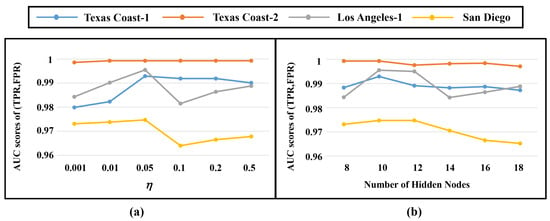
Figure 4.
Implementation details on four HSIs. (a) The threshold . (b) Number of hidden nodes.
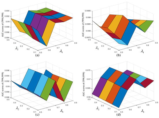
Figure 5.
Implementation details of the hyperparameters and on (a) Texas Coast-1, (b) Texas Coast-2, (c) Los Angeles and (d) San Diego. Different colors refer to different intervals of values of and .
4.2. Detection Performance
We compare RANet with seven frequently cited and state-of-the-art approaches, including RX [18], LRASR [23], LSMAD [22], SSDF [43], LSDM–MoG [44], PTA [45], PAB–DC [46], Auto-AD [33] and 2S–GLRT [47]. Reed Xiaoli (RX) algorithm is proposed assuming that the background obeys multi-variate Gaussian normal distribution. LRASR is a hyperspectral anomaly detection method based on the existence of mixed pixels, which assumes that background data is located in multiple low-rank subspaces. LSMAD realizes anomaly detection by decomposing hyperspectral data into low-rank background components and sparse anomaly components. SSDF is a forest discriminant method based on subspace selection for hyperspectral anomaly detection. LSDM–MoG is a low-rank sparse decomposition method based on a mixed Gaussian model for HAD. PTA proposed a tensor approximation method based on priors. PAB–DC is an HAD method based on low rank and sparse representation strategy. Auto-AD is a kind of method based on an autonomous hyperspectral anomaly detection network. 2S–GLRT proposes an adaptive detector based on generalized likelihood ratio test (GLRT). All of the methods above are reimplemented according to their papers and open-source codes.
In order to visually demonstrate the detection performance, Figure 6 displays the visual detection maps of the four HSIs under the above-mentioned methods. It is worth noting that RANet can completely and accurately detect anomalies of different sizes and locations, while other methods have problems such as false detection, missed detection and blurred targets to varying degrees. In addition, RANet can effectively suppress strip noise, thereby achieving good performance.
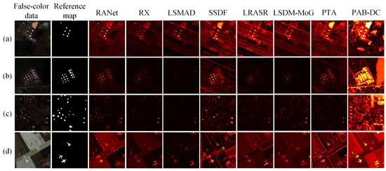
Figure 6.
False-color data, reference map, and detection maps of the compared methods for (a) Texas Coast-1, (b) Texas Coast-2, (c) Los Angeles and (d) San Diego.
By quantitatively comparing these detectors, Table 1 lists the AUC scores of (TPR, FPR) of the seven popular methods and RANet on the four real HSIs. Notably, the AUC scores of (TPR, FPR) are consistent with the visual detection maps in Figure 6. It can be observed that RANet outperforms other methods with the highest AUC score of (TPR, FPR) on every HSI.

Table 1.
AUC scores of (TPR, FPR) for the compared methods on different datasets. The scores in bold form refer to the best performance.
To further demonstrate the detection performance among compared methods and RANet, we plot the ROC curves of (TPR, FPR) of eight approaches on the four HSIs. As shown in Figure 7, the ROC curves of (TPR, FPR) of RANet lie nearer the top-left corner, and it is obvious that RANet can obtain a high probability of detection and provide the most excellent detection performance. As for RX, its curve is also very close to the upper left corner, but it still does not catch up with RANet’s detection effect due to missing some objects. For other methods, they all show defects on different datasets, resulting in poor performance of the ROC curves.

Figure 7.
ROC curves of (TPR, FPR) for the algorithms on (a) Texas Coast-1, (b) Texas Coast-2, (c) Los Angeles and (d) San Diego.
Meanwhile, we employ the Box–Whisker Plots to analyze the ability to separate the anomalies and background and then observe the effect of suppressing the background. As illustrated in Figure 8, the detection results of each method correspond to two boxes, in which the red box represents the distribution range of anomaly detection values and the blue box represents the distribution range of background detection values. The relative positions and compactness of the boxes reflect the trends in background and anomalous pixel distributions. In general, RANet can evidently reveal the capability of discriminating anomaly and background.
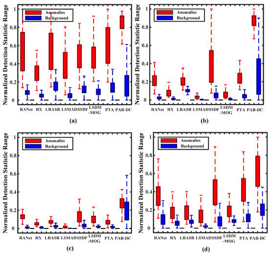
Figure 8.
Background–anomaly separation analysis of the compared methods on (a) Texas Coast-1, (b) Texas Coast-2, (c) Los Angeles and (d) San Diego.
4.3. Discussion
In this section, we conduct experiments to discuss four factors related to the performance of RANet’s framework.
Network Architecture. In order to explore the training performance of the reconstructed backbone, we adopt AE, CAE and both CAE and TA modules (CAE + TA) separately. As shown in Figure 9a, it is obvious that, with joint learning of CAE + TA, the framework achieves the most satisfying detection result. Since AE performs anomaly detection by extracting the hidden layer features of each spectral vector without considering the correspondence between similar spectra, it does not obtain high detection results. Instead, CAE takes advantage of local spectral similarity, which makes its detection performance better than AE. For all datasets, the detection results illustrate the effectiveness of the TA module.
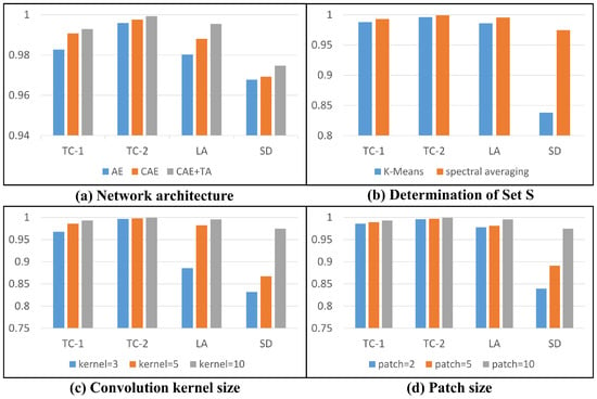
Figure 9.
Detection accuracy comparison under four factors related to the performance of RANet on four HSIs.
Determination of Set . As shown in Figure 9b, we compare the effectiveness of the classical clustering algorithm K-Means and spectral averaging for the set . As the most classical clustering method, K-Means aims to select the most representative samples. In RANet, we perform clustering on each cube and select a representative vector for each cube. It is worth noting that spectral averaging is slightly better than K-Means clustering for the Texas Coast-1 dataset, Texas Coast-2 dataset and Los Angeles dataset. As for the San Diego dataset, spectral averaging shows superior performance than K-Means clustering, which indicates that spectral averaging can obtain a more suitable set to make the performance of the TA module fully utilized.
Convolution Kernel Size. As one of the most important parameters in CAE, the size of the convolution kernel greatly affects the performance of the network. Therefore, we conduct an experiment to analyze the selection of the size of the convolution kernel. As shown in Figure 9c, we set the convolution kernel size to 3, 5 and 10 to analyze the impact on the detection results. It can be seen that the performance continues to improve with the increase in the convolution kernel and, when the size of the convolution kernel is 10, the performance is superior. Although the improvement in performance is small on the Texas Coast-1 dataset and Texas Coast-2 dataset, it is high on the Los Angeles dataset and San Diego dataset. Consequently, we adopt a convolution kernel size of 10.
Size of 3D Cube. As defined in Section 3, the size of each cube determines the number of cubes, which in turn determines the detection performance of RANet. Hence, it is necessary to conduct an experiment to determine the size of a 3D cube. As shown in Figure 9d, we measure the detection performance when the cube size is set to 2, 5 and 10. The experiments show that the performance tends to be more competitive as the cube size increases and all the datasets achieve satisfactory performance with a cube size 10. Since the four HSIs all contain 100 × 100 pixels, the number of cubes P is 100.
5. Conclusions and Future Work
In this paper, we propose a novel framework named RANet for HAD. The main intent of our method is to achieve relationship attention-guided unsupervised learning with CAE. First of all, RANet leverages an attention-based architecture with a customized incidence matrix to learn deep topological relationships from HSIs. Second, an unsupervised CAE is designed as the reconstructed backbone with high-fidelity high-dimensional data representations. Third, the reconstructed backbone and topological attention are jointly learned to obtain reconstructed hyperspectral images. Finally, the reconstruction error is used to detect anomalies. Extensive experiments are conducted to validate that our RANet has competitive performance when compared to state-of-the-art approaches. In the future, we plan to work on improving the way we build our models to reconstruct equally good models with less computation or fewer resources.
Author Contributions
Conceptualization, Y.S. and Y.L. (Yang Liu); methodology, Y.S. and X.G.; software, Y.S. and L.L.; validation, Y.W. and Y.Y.; writing—original draft preparation, Y.S. and Y.L. (Yunsong Li); writing—review and editing, Y.D. and M.Z.; supervision, Y.L. (Yunsong Li). All authors have read and agreed to the published version of the manuscript.
Funding
This work was supported by the National Natural Science Foundation of China under Grant 62121001.
Data Availability Statement
No new data were created.
Conflicts of Interest
The authors declare no conflict of interest.
References
- Veganzones, M.A.; Tochon, G.; Dalla-Mura, M.; Plaza, A.J.; Chanussot, J. Hyperspectral image segmentation using a new spectral unmixing-based binary partition tree representation. IEEE Trans. Image Process. 2014, 23, 3574–3589. [Google Scholar] [CrossRef]
- Dong, W.; Fu, F.; Shi, G.; Cao, X.; Wu, J.; Li, G.; Li, X. Hyperspectral image super-resolution via non-negative structured sparse representation. IEEE Trans. Image Process. 2016, 25, 2337–2352. [Google Scholar] [CrossRef]
- Akgun, T.; Altunbasak, Y.; Mersereau, R. Super-resolution reconstruction of hyperspectral images. IEEE Trans. Image Process. 2005, 14, 1860–1875. [Google Scholar] [CrossRef]
- Wang, L.; Zhang, T.; Fu, Y.; Huang, H. Hyperreconnet: Joint coded aperture optimization and image reconstruction for compressive hyperspectral imaging. IEEE Trans. Image Process. 2019, 28, 2257–2270. [Google Scholar] [CrossRef]
- Veganzones, M.A.; Simões, M.; Licciardi, G.; Yokoya, N.; Bioucas-Dias, J.M.; Chanussot, J. Hyperspectral super-resolution of locally low rank images from complementary multisource data. IEEE Trans. Image Process. 2016, 25, 274–288. [Google Scholar] [CrossRef]
- Jiang, K.; Xie, W.; Lei, J.; Jiang, T.; Li, Y. Lren: Low-rank embedded network for sample-free hyperspectral anomaly detection. AAAI-AAAI Conf. Artif. Intell. 2021, 35, 4139–4146. [Google Scholar] [CrossRef]
- Wu, H.; Prasad, S. Semi-supervised deep learning using pseudo labels for hyperspectral image classification. IEEE Trans. Image Process. 2018, 27, 1259–1270. [Google Scholar] [CrossRef] [PubMed]
- Yang, S.; Shi, Z. Hyperspectral image target detection improvement based on total variation. IEEE Trans. Image Process. 2016, 25, 2249–2258. [Google Scholar] [CrossRef] [PubMed]
- Imbiriba, T.; Bermudez, J.C.M.; Richard, C.; Tourneret, J.-Y. Nonparametric detection of nonlinearly mixed pixels and endmember estimation in hyperspectral images. IEEE Trans. Image Process. 2016, 25, 1136–1151. [Google Scholar] [CrossRef]
- Du, B.; Zhang, Y.; Zhang, L.; Tao, D. Beyond the sparsity-based target detector: A hybrid sparsity and statistics-based detector for hyperspectral images. IEEE Trans. Image Process. 2016, 25, 5345–5357. [Google Scholar] [CrossRef]
- Altmann, Y.; Dobigeon, N.; McLaughlin, S.; Tourneret, J.-Y. Residual component analysis of hyperspectral images—Application to joint nonlinear unmixing and nonlinearity detection. IEEE Trans. Image Process. 2014, 23, 2148–2158. [Google Scholar] [CrossRef] [PubMed]
- Li, Z.; Zhang, Y. Hyperspectral anomaly detection via image super-resolution processing and spatial correlation. IEEE Trans. Geosci. Remote Sens. 2021, 59, 2307–2320. [Google Scholar] [CrossRef]
- Wang, S.; Wang, X.; Zhong, Y.; Zhang, L. Hyperspectral anomaly detection via locally enhanced low-rank prior. IEEE Trans. Geosci. Remote Sens. 2020, 58, 6995–7009. [Google Scholar] [CrossRef]
- Tu, B.; Yang, X.; Zhou, C.; He, D.; Plaza, A. Hyperspectral anomaly detection using dual window density. IEEE Trans. Geosci. Remote Sens. 2020, 58, 8503–8517. [Google Scholar] [CrossRef]
- Liu, J.; Feng, Y.; Liu, W.; Orlando, D.; Li, H. Training data assisted anomaly detection of multi-pixel targets in hyperspectral imagery. IEEE Trans. Signal Process. 2020, 68, 3022–3032. [Google Scholar] [CrossRef]
- Zhang, W.; Lu, X.; Li, X. Similarity constrained convex nonnegative matrix factorization for hyperspectral anomaly detection. IEEE Trans. Geosci. Remote Sens. 2019, 57, 4810–4822. [Google Scholar] [CrossRef]
- Dong, G.; Liao, G.; Liu, H.; Kuang, G. A review of the autoencoder and its variants: A comparative perspective from target recognition in synthetic-aperture radar images. IEEE Geosci. Remote Sens. Mag. 2018, 6, 44–68. [Google Scholar] [CrossRef]
- Reed, I.S.; Yu, X. Adaptive multiple-band cfar detection of an optical pattern with unknown spectral distribution. IEEE Trans. Acoust. Speech Signal Process. 1990, 38, 1760–1770. [Google Scholar] [CrossRef]
- Matteoli, S.; Veracini, T.; Diani, M.; Corsini, G. A locally adaptive background density estimator: An evolution for rx-based anomaly detectors. IEEE Geosci. Remote Sens. Lett. 2014, 11, 323–327. [Google Scholar] [CrossRef]
- Li, W.; Du, Q. Collaborative representation for hyperspectral anomaly detection. IEEE Trans. Geosci. Remote Sens. 2015, 53, 1463–1474. [Google Scholar] [CrossRef]
- Li, J.; Zhang, H.; Zhang, L.; Ma, L. Hyperspectral anomaly detection by the use of background joint sparse representation. IEEE J. Sel. Top. Appl. Earth Observ. Remote Sens. 2015, 8, 2523–2533. [Google Scholar] [CrossRef]
- Zhang, Y.; Du, B.; Zhang, L.; Wang, S. A low-rank and sparse matrix decomposition-based mahalanobis distance method for hyperspectral anomaly detection. IEEE Trans. Geosci. Remote Sens. 2016, 54, 1376–1389. [Google Scholar] [CrossRef]
- Xu, Y.; Wu, Z.; Li, J.; Plaza, A.; Wei, Z. Anomaly detection in hyperspectral images based on low-rank and sparse representation. IEEE Trans. Geosci. Remote Sens. 2016, 54, 1990–2000. [Google Scholar] [CrossRef]
- Wang, K.; Gou, C.; Duan, Y.; Lin, Y.; Zheng, X.; Wang, F.-Y. Generative adversarial networks: Introduction and outlook. IEEE/CAA J. Autom. Sin. 2017, 4, 588–598. [Google Scholar] [CrossRef]
- Li, W.; Wu, G.; Du, Q. Transferred deep learning for anomaly detection in hyperspectral imagery. IEEE Geosci. Remote Sens. Lett. 2017, 14, 597–601. [Google Scholar] [CrossRef]
- Liu, G.; Lin, Z.; Yan, S.; Sun, J.; Yu, Y.; Ma, Y. Robust recovery of subspace structures by low-rank representation. IEEE Trans. Pattern Anal. Mach. Intell. 2013, 35, 171–184. [Google Scholar] [CrossRef] [PubMed]
- Abati, D.; Porrello, A.; Calderara, S.; Cucchiara, R. Latent space autoregression for novelty detection. In Proceedings of the 2019 IEEE/CVF Conference on Computer Vision and Pattern Recognition (CVPR), Long Beach, CA, USA, 15–20 June 2019; pp. 481–490. [Google Scholar] [CrossRef]
- Park, H.; Noh, J.; Ham, B. Learning memory-guided normality for anomaly detection. In Proceedings of the 2020 IEEE/CVF Conference on Computer Vision and Pattern Recognition (CVPR), Seattle, WA, USA, 14–19 June 2020; pp. 14360–14369. [Google Scholar] [CrossRef]
- Pang, G.; Yan, C.; Shen, C.; Hengel, A.V.; Bai, X. Self-trained deep ordinal regression for end-to-end video anomaly detection. In Proceedings of the 2020 IEEE/CVF Conference on Computer Vision and Pattern Recognition (CVPR), Seattle, WA, USA, 14–19 June 2020; pp. 12170–12179. [Google Scholar] [CrossRef]
- Xie, W.; Lei, J.; Liu, B.; Li, Y.; Jia, X. Spectral constraint adversarial autoencoders approach to feature representation in hyperspectral anomaly detection. Neural Netw. 2019, 119, 222–234. [Google Scholar] [CrossRef]
- Liu, Y.; Xie, W.; Li, Y.; Li, Z.; Du, Q. Dual-frequency autoencoder for anomaly detection in transformed hyperspectral imagery. IEEE Trans. Geosci. Remote Sens. 2022, 60, 5523613. [Google Scholar] [CrossRef]
- Xie, W.; Fan, S.; Qu, J.; Wu, X.; Lu, Y.; Du, Q. Spectral distribution-aware estimation network for hyperspectral anomaly detection. IEEE Trans. Geosci. Remote Sens. 2021, 60, 5512312. [Google Scholar] [CrossRef]
- Wang, S.; Wang, X.; Zhang, L.; Zhong, Y. Auto-ad: Autonomous hyperspectral anomaly detection network based on fully convolutional autoencoder. IEEE Trans. Geosci. Remote Sens. 2021, 60, 1–14. [Google Scholar] [CrossRef]
- Jiang, T.; Xie, W.; Li, Y.; Lei, J.; Du, Q. Weakly supervised discriminative learning with spectral constrained generative adversarial network for hyperspectral anomaly detection. IEEE Trans. Neural Netw. Learn. Syst. 2021, 33, 6504–6517. [Google Scholar] [CrossRef] [PubMed]
- Jiang, T.; Li, Y.; Xie, W.; Du, Q. Discriminative reconstruction constrained generative adversarial network for hyperspectral anomaly detection. IEEE Trans. Geosci. Remote Sens. 2020, 58, 4666–4679. [Google Scholar] [CrossRef]
- Fu, X.; Jia, S.; Zhuang, L.; Xu, M.; Zhou, J.; Li, Q. Hyperspectral anomaly detection via deep plug-and-play denoising cnn regularization. IEEE Trans. Geosci. Remote Sens. 2021, 59, 9553–9568. [Google Scholar] [CrossRef]
- Ma, J.; Xie, W.; Li, Y.; Fang, L. Bsdm: Background suppression diffusion model for hyperspectral anomaly detection. arXiv 2023, arXiv:2307.09861. [Google Scholar]
- Wang, M.; Wang, Q.; Hong, D.; Roy, S.K.; Chanussot, J. Learning tensor low-rank representation for hyperspectral anomaly detection. IEEE Trans. Cybern. 2023, 53, 679–691. [Google Scholar] [CrossRef]
- Jiang, K.; Xie, W.; Lei, J.; Li, Z.; Li, Y.; Jiang, T.; Du, Q. E2e-liade: End-to-end local invariant autoencoding density estimation model for anomaly target detection in hyperspectral image. IEEE Trans. Cybern. 2021, 52, 11385–11396. [Google Scholar] [CrossRef]
- Zweig, M.H.; Campbell, G. Receiver-operating characteristic (roc) plots: A fundamental evaluation tool in clinical medicine. Clin. Chem. 1993, 39, 561–577. [Google Scholar] [CrossRef] [PubMed]
- Flach, P.; Hernándezorallo, J.; Ferri, C. A coherent interpretation of aucas a measure of aggregated classification performance. In Proceedings of the 28th International Conference on Machine Learning (ICML-11), Bellevue, WA, USA, 28 June–2 July 2011; pp. 657–664. [Google Scholar]
- Mcgill, R.; Tukey, J.W.; Larsen, W.A. Variation of box plots. Am. Stat. 1978, 32, 12–16. [Google Scholar]
- Chang, S.; Du, B.; Zhang, L. A subspace selection-based discriminative forest method for hyperspectral anomaly detection. IEEE Trans. Geosci. Remote Sens. 2020, 58, 4033–4046. [Google Scholar] [CrossRef]
- Li, L.; Li, W.; Du, Q.; Tao, R. Low-rank and sparse decomposition with mixture of gaussian for hyperspectral anomaly detection. IEEE Trans. Cybern. 2021, 51, 4363–4372. [Google Scholar] [CrossRef]
- Li, L.; Li, W.; Qu, Y.; Zhao, C.; Tao, R.; Du, Q. Prior-based tensor approximation for anomaly detection in hyperspectral imagery. IEEE Trans. Neural Netw. Learn. Syst. 2022, 33, 1037–1050. [Google Scholar] [CrossRef]
- Huyan, N.; Zhang, X.; Zhou, H.; Jiao, L. Hyperspectral anomaly detection via background and potential anomaly dictionaries construction. IEEE Trans. Geosci. Remote Sens. 2019, 57, 2263–2276. [Google Scholar] [CrossRef]
- Liu, J.; Hou, Z.; Li, W.; Tao, R.; Orlando, D.; Li, H. Multipixel anomaly detection with unknown patterns for hyperspectral imagery. IEEE Trans. Neural Netw. Learn. Syst. 2022, 33, 5557–5567. [Google Scholar] [CrossRef]
Disclaimer/Publisher’s Note: The statements, opinions and data contained in all publications are solely those of the individual author(s) and contributor(s) and not of MDPI and/or the editor(s). MDPI and/or the editor(s) disclaim responsibility for any injury to people or property resulting from any ideas, methods, instructions or products referred to in the content. |
© 2023 by the authors. Licensee MDPI, Basel, Switzerland. This article is an open access article distributed under the terms and conditions of the Creative Commons Attribution (CC BY) license (https://creativecommons.org/licenses/by/4.0/).