Retrieval of Land Surface Temperature over Mountainous Areas Using Fengyun-3D MERSI-II Data

Abstract

Land surface temperature (LST) is an important physical quantity in the energy exchange of hydrothermal cycles between the land and near-surface atmosphere at regional and global scales. However, the traditional thermal infrared transfer equation (RTE) and LST retrieval algorithms are always based on the underlying assumptions of homogeneity and isotropy, which ignore the terrain effect influence of a heterogeneous topography. It can cause significant errors when traditional RTE and other algorithms are used to retrieve LST in such mountainous research. In this study, the mountainous thermal infrared transfer model considering terrain effect correction is used to retrieve the mountainous LST using FY-3D MERSI-II data, and the in situ site data are simultaneously utilized to evaluate the performance of the iterative single-channel algorithm. The elevation of this study region ranges from 500 m to 2200 m, whereas the minimum SVF can reach 0.75. Results show that the spatial distribution of the retrieved LST is similar to topographic features, and the LST has larger values in the lower valley and smaller values in the higher ridge. In addition, the overall bias and RMSE between the retrieved LSTs and five in situ stations are respectively −0.70 K and 2.64 K, which demonstrates this iterative single-channel algorithm performs well in taking into account the terrain effect influence. Accuracy of the LST estimation is meaningful for mountainous ecological environmental monitoring and global climate research. Such an adjacent terrain effect correction should be considered in future research on complex terrains, especially with high spatial resolution TIR data.

1. Introduction

Land surface temperature (LST) is an essential quantity in the study of surface heat transfer, the environment, and meteorological and ecological research. It is widely used for research on the water cycle and evaporation [1,2,3], drought monitoring [4,5,6], the urban heat island effect [7,8,9,10], and global climate monitoring [11,12,13]. The current LST retrieval algorithm includes the single-channel algorithm, split-window algorithm, temperature-emissivity separation algorithm, and multi-angle algorithm [14,15]. Most of these algorithms retrieve the LST by the hypothesis of homogenous and isotropic land surfaces without considering terrain reliefs. However, it is inaccurate to retrieve the LST with these assumptions using a traditional radiative transfer equation (RTE) in regions of complex topography, and such a such can cause significant errors [16]. Mountainous complex terrains account for 24% of global regions and 69% of China [17], and their topography makes the thermal radiation transfer more complex and uncertain. Meanwhile, the LST is the direct reflection of heat transfer, which can even control the degree of ablation in mountainous snow surfaces and glaciers [18]. Thus, it is urgent to develop the retrieval algorithm of the mountainous surface temperature.

In recent years, terrain-corrected radiative variables have been frequently proposed to obtain more accurate land surface parameters [19], and many terrain correction models have been developed to eliminate the quantitative influence of radiative transfer from the topography. Initially, many physical models utilized the solar–terrain–satellite geometry to calculate terrain correction factors, and they were simply applied to the acquisition of mountainous remote sensing images by optical satellites [20]. The result was a 30% overestimation of the multiple reflections when the study areas are selected in snow targets over high-relief areas [21,22], and larger slopes and aspects can introduce 60% errors at the in situ albedo measurement [23]. A mountainous 3-dimensional surface makes the radiative transfer process more complex, and topographic shading can affect the energy balance of a complex terrain [24]. The significance of the topography effect correction is also highlighted in shortwave and longwave radiation research over mountainous areas [25]. The solar direct radiation and atmospheric radiation from the hemispheric direction are obstructed by a heterogeneous terrain, which causes underestimation of the total radiation received by the land surface. Wang et al. pointed out that the invisibility of some targets leads to significant errors in quantifying solar direct radiation, and the adjacent effects should be corrected in mountainous terrains [26]. In addition, the topographic effect causes the overestimation of downward radiation when simple extrapolation methods are applied under different spatiotemporal conditions, and it cannot be ignored when the spatial resolution is coarser than 5000 m [27,28].

Complex topographic structures decrease the atmospheric downward radiation from hemispherical space, whereas it can increase the total thermal radiation via the adjacent terrain radiation. The heterogeneity of mountainous brightness temperature can reach 9 K when the terrain is coupled with solar and viewing geometries [29]. The terrain effect has been analyzed via various satellite thermal channels [30]. Ignoring the terrain effect would cause large satellite-viewing biases in LST retrieval over rugged terrains [31,32]. More terrain effect correction models should be developed to reduce the LST retrieval bias over complex terrains. Motivated by quantitative research in mountainous regions, Wu et al. utilized the single-channel algorithm considering the terrain to retrieve Qiyi glacier surface temperatures, and analyzed the adjacent terrain radiation, which is 2.6 times the atmospheric downward radiation over the glacier tongue areas [16,17]. The iterative single-channel retrieval algorithm is proposed to obtain the Tibetan plateau LST and is validated by the Discrete Anisotropic Radiative Transfer (DART) forward simulation, which demonstrated that the terrain effect incurs approximately 1 K errors in the deep valley [33]. In addition, the LST normalization (energy balance- and random forest-based methods) of the terrain frequently is important to obtain a high accuracy LST with a terrain correction [34,35,36]. The above research shows that the terrain effect correction is important for radiative parameters (reflectance, atmospheric shortwave and longwave radiation, and LST), and more land surface parameter retrieval algorithms should be noticed and developed over complex terrain areas.

Therefore, the terrain effect correction must be taken into account for the retrieval of the LST in mountainous areas. This study utilized the mountainous thermal infrared radiation equation (MRTE) considering the terrain effect correction, and retrieved the LST by an iterative algorithm using FY-3D MERSI-II data. The study areas are shown in Section 2. Section 3 introduces the MRTE and LST retrieval methodology. Section 4 displays and analyzes the retrieved results for the mountainous LST. Finally, Section 5 discusses the retrieval algorithm and summarizes the conclusions of this study.

2. Study Area and Material

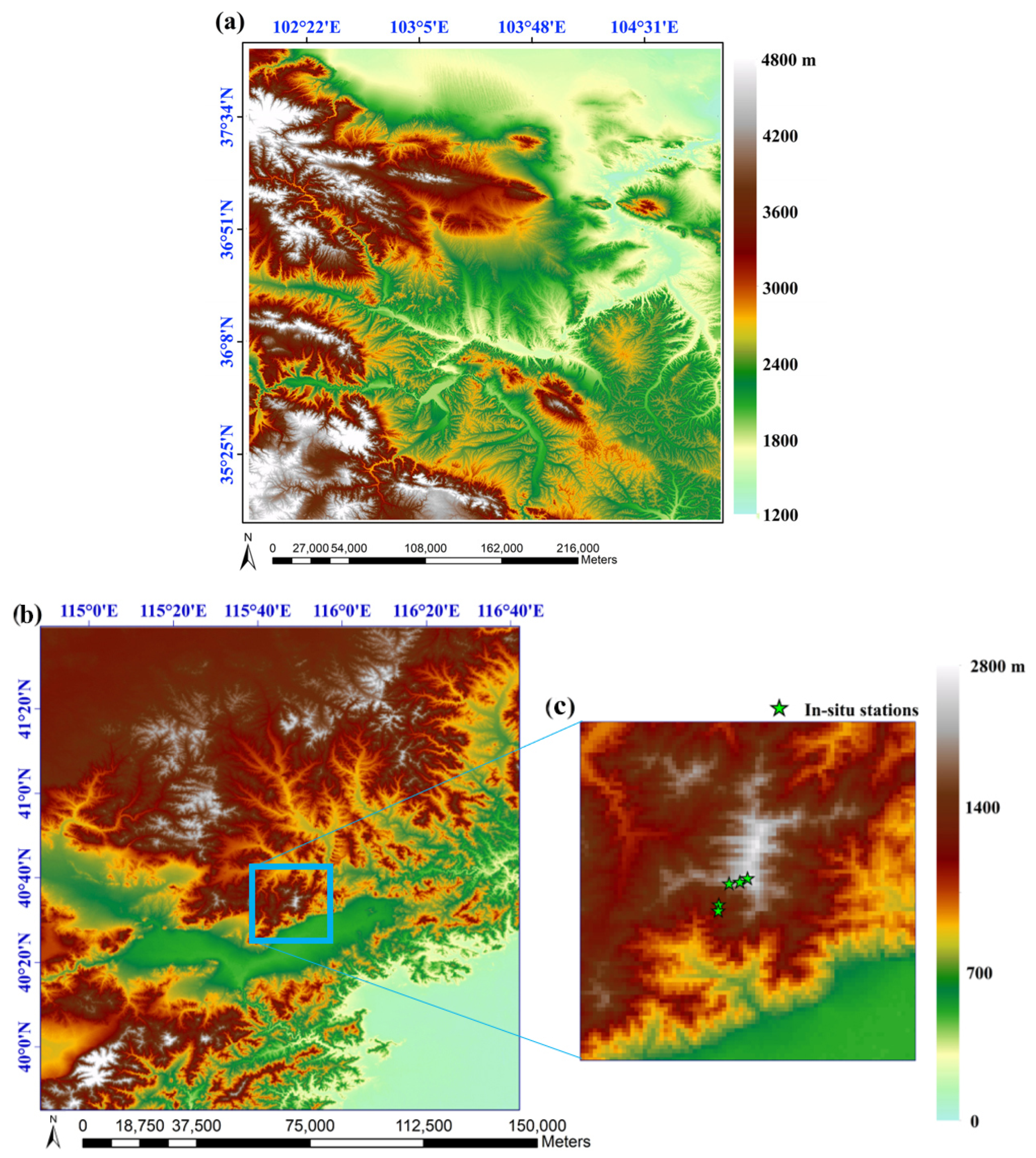
2.1. Study Areas

In this study, two regions with different topographic features were selected as illustrations for retrieving the LST using an iterative single-channel algorithm, which is used to verify the generalizability of the algorithm. Study area-I is part of Kunlun Mountain, and its spatial extent covers latitudes from 35.00°N to 38.00°N and longitudes from 102.00°E to 105.00°E. It is continually influenced by the atmospheric air mass, and the air temperature fluctuates strongly in this region. Its special location makes it immune to the monsoon climate of the Pacific and Indian Oceans. The maximum elevation reaches 4800 m, whereas its lowest elevation is 1200 m. There is a higher height difference than study area-II in this region. The north-east direction is relatively flat, and the steep hills can be found in the western part.

Study area-II is located in the Yanqing Zone, northwest of Beijing, China. Its spatial extent covers latitudes from 39.00°N to 42.00°N and longitudes from 114.00°E to 117.00°E. This region has a continental monsoon climate with cool summers and winters, and is the transition zone between high-temperature and middle-temperature zones, and semi-arid and semi-humid zones. The district covers 1993 km² with an average altitude of 500 m, and the Haituo Mountain is the highest peak, with an elevation of 2241 m. Its three sides are surrounded by mountains (north and southeast), and mountains account for 74% of the coverage area. Therefore, these two regions are suitable for the retrieval of the LST considering the terrain effect corrections with different topographic features. The location and elevation images of study area-I and area-II are respectively shown in Figure 1a,b. There are five in situ sites in study area-II, whose locations and elevations are shown in Figure 1c. They are used to evaluate the performance of LST retrieval algorithm in Section 4.

2.2. FY-3D Data

Fengyun-3D (FY-3D) is the fourth satellite of the Fengyun series, and it was launched on 15 November 2017 at Taiyuan Satellite Launch Center, China. This polar-orbiting satellite carries the Medium Resolution Spectral Imager (MERSI)-II, and the ground application system of Fengyun-3D consists of a global data acquisition station network with ground stations at the North and South Poles plus four domestic ground stations, for the first time realizing two-hour global complete detection data acquisition. There are 25 channels whose spectral ranges from 0.412 to 12 μm, including two spatial resolutions of 250 m and 1000 m. The center wavelengths of the two thermal infrared spectra are respectively 10.8 μm for band 24 and 12.0 μm for band 25, which can be downloaded at http://satellite.nsmc.org.cn/PortalSite/Data/Satellite.aspx (accessed on 1 January 2019). Their spectral response functions are shown in Figure 2. In this study, the thermal infrared radiance of band 24 (250 m) is used to retrieve the LST by using the single-channel algorithm with a noise equivalent temperature difference (NETD) of 0.4 K. Band 2 (red) and band 4 (near-infrared) are used to obtain the normalization vegetation index (NDVI) at the FY-3D satellite transit time, and they are further used to calculate the land surface emissivity (LSE) by the NDVI threshold method.

2.3. NCEP Data

The Global Forecast System (GFS) yields the atmospheric reanalysis profile data released by NCEP in 2007, and it uses the most advanced global assimilation system and a comprehensive database [37]. These atmospheric data include temperature profiles, relative humidity profiles, and ozone profiles with 31 atmospheric pressure layers, including 1, 2, 3, 5, 7, 10, 20, 30, 50, 70, 100, 150, 200, 250, 300, 350, 400, 450, 500, 550, 600, 650, 700, 750, 800, 850, 900, 925, 950, 975, and 1000 hpa. Globally, the spatial resolution of the data is 0.5° × 0.5° in version 004, and they are available for the hours of 00, 06, 12, and 18 (UTC time) from January 2007 to the present. These data can be downloaded from https://www.ncdc.noaa.gov/data-access/model-data/model-datasets/global-forcast-system-gfs (accessed on 1 January 2019). In this study, the GFS atmospheric profiles are interpolated by the latitude, longitude, and elevation of FY-3D at pixel scale (250 m), then they are entered into MODTRAN 5.2 to obtain the atmospheric upwelling radiance, atmospheric downwelling radiance, and atmospheric transmittance.

2.4. ASTER GED Data

The ASTER Global Emissivity Dataset (GED) released in 2004 was developed by the NASA Jet Propulsion Laboratory (JPL) [38]. It provides global emissivity maps, which were generated by the TES algorithm using all available clear-sky ASTER scenes from 2000 to 2008 [39]. Meanwhile, it was produced with a spatial resolution of 1° × 1° with two scales (100 m and 1000 m), and the database with 100 m spatial resolution is utilized in this study to match the FY-3D radiance. This database includes the emissivity with respect to five bands of ASTER, elevation, latitude, and longitude per pixel. In this study, the ASTER GED is used to obtain the bare soil emissivity by using the NDVI threshold method.

2.5. Digital Elevation Model (DEM) Data

The NASA DEM is an improved version of the Shuttle Radar Topography Mission (SRTM) released by NASA in February 2020, whose missing values are filled with ASTER GED data with improved accuracy. The NASA DEM is available for 80% of all the Earth’s land masses, which are between 60°N and 56°S latitude, and its spatial resolution is 1 arc-second (~30 m). It can be downloaded from https://search.earthdata.nasa.gov/ (accessed on 13 February 2020). In this study, the NASA DEM is used to extract the topographic landforms. The slope angle and aspect angle are calculated via the inverse distance squared weighted difference method [40], and the sky-view factor (SVF) is calculated via the method of [41].

3. Methodology

With the assumption of a homogenous underlying thermal infrared radiation (TIR) received by sensors at the top of the atmosphere (TOA), this radiation can be divided into three parts: (1) L_emi surface emitting radiation, (2) L_up atmospheric upwelling radiation, and (3) L_dw atmospheric downwelling radiation. The thermal infrared radiative equation (RTE) can be written as:

$$L_{TOA}=\epsilon B(T_s)\tau +\left(1-\epsilon \right)L_{dw}\tau +L_{up}$$

(1)

where L_TOA is the thermal infrared radiance at the TOA, ε is the land surface emissivity, τ is the atmospheric transmittance, and T_s is the land surface temperature in flat regions without the terrain correction effect.

Due to the geometric structures of the various terrains, the mountainous radiative transfer equation is distinctly different from that of homogeneous and flat regions. It is undoubtedly the case that the mountainous radiative transfer equation in the TIR field will be more complex than that in flat regions via the multi-scattering radiation induced by mountainous surfaces. In fact, the parts obscured by the terrain will decrease the atmospheric downwelling radiation, whereas the total thermal radiation is increased by the surrounding terrain emitting thermal radiation [33]. Therefore, the atmospheric downwelling radiance can be respectively written as Equation (2) at the TOA of mountainous areas:

$$L_{TOA}^{dw}=V_d(1-\epsilon )L_{dw}\tau$$

(2)

where $L_{TOA}^{dw}$ is the atmospheric downwelling radiance at the TOA in mountainous areas, V_d is the sky-view factor (SVF), which ranges from 0 to 1, and which represents the visible ratios of the hemisphere atmospheric radiation to the target pixel [41]. Its equation is written as:

$$V_d\approx \frac{1}{2\pi }{\displaystyle {\int }_0^{2\pi }[}\cos S{\sin }^2{H}_{\varphi }+\sin S\cos \left(\varphi -A\right)\times \left(H_{\varphi }-\sin H_{\varphi }\cos H_{\varphi }\right)]d\varphi$$

(3)

where S is the slope angle, A is the aspect angle, ϕ is the searching azimuthal angle, and H_ϕ is the horizontal angle, which is the angle between the normal line of the horizontal plane and the line which connects the target pixel and surrounding pixels. The search range of this study area is determined as 5 km, and there are 16 search directions, which are 0°, 30°, 45°, 60°, 90°, 120°, 135°, 150°, 180°, 210°, 225°, 240°, 270°, 300°, 315°, and 330°. In addition, the S and A are calculated by a third-order inverse distance squared weighted difference method [40].

On the other hand, the surrounding environmental radiation of the target pixel can be represented as the sum radiation of available adjacent pixels (L_adj); thus, the adjacent terrain radiation can be written as:

$$L_{TOA}^{adj}=(1-\epsilon )L_{adj}\tau$$

(4)

where $L_{TOA}^{adj}$ is the adjacent terrain radiance at the TOA in mountainous areas. L_adj can be written as [42]:

$$L_{adj}={\displaystyle \sum _{j=1}^N\frac{L_{Pj}\cos T_M\cos T_{Pj}d{S}_{Pj}}{\pi r_{MPj}^2}}$$

(5)

with

$$L_{Pj}={\epsilon }_{j}B(T_{sj})+(1-{\epsilon }_j)V_{dj}{L}_{adj,j}$$

(6)

where subscripts M and P represent the target pixel and surrounding pixel, respectively, j represents the jth surrounding pixel, N is the number of surrounding pixels visible to the target pixel, L_P is the radiation from surrounding pixels, T_M is the angle between the slope normal line of the target pixel M and the line M_P, T_P is the angle between the slope normal line of the surrounding pixel P and the line M_P, dS_P is the slope area of the surrounding pixel P, and r_MP is the distance between the target pixel M and the surrounding pixel P.

Due to the influence of the topography in mountainous areas, the sky-view factor and adjacent terrain radiation are utilized to obtain the mountainous radiative transfer equation, which can be written as follows [33]:

$$L_{TOA,m}=\epsilon B(T_{s,m})\tau +V_d\left(1-\epsilon \right)L_{dw}\tau +\left(1-\epsilon \right)L_{adj}\tau +L_{up}$$

(7)

where L_TOA,m is the thermal infrared radiance at the TOA in mountainous areas, and T_s,m is the LST in mountainous surfaces with the terrain correction effect.

Based on this mountainous radiative transfer equation, the single-channel algorithm is used to retrieve the LST in mountainous areas in this study, with reference to [33]. By reversing Equation (7), the mountainous radiative transfer equation with the terrain correction effect is written as:

$$T_{s,m}=B^{-1}\left[\frac{L_{TOA,m}-L_{up}-(1-\epsilon )\tau L_{dw}{V}_d-(1-\epsilon )\tau L_{adj}}{\epsilon \tau }\right]$$

(8)

where B⁻¹ is the inverse Planck function.

To retrieve the LST with the terrain correction effect by Equation (8), the atmospheric upwelling radiance, atmospheric downwelling radiance, and atmospheric transmittance can be obtained from MODTRAN by inputting the NCEP atmospheric profiles with a temporal-spatial interpolation. The land surface emissivity is calculated by the NDVI threshold method utilizing the ASTER GED products and FY-3D MERSI-II in the near-infrared and red bands. The SVF is calculated with NASA DEM data by Equation (3). Even if the other parameters are known in advance for the target pixel, the acquisition of the adjacent terrain radiance is still difficult when the LST of adjacent pixels is unknown. Therefore, the retrieved LST from the RTE is used as the original input of Equation (8), and the reversing Equation (1) is written as:

$$T_s=B^{-1}\left[\frac{L_{TOA}-L_{up}-(1-\epsilon )\tau L_{dw}}{\epsilon \tau }\right]$$

(9)

To obtain a reasonable and accurate LST in mountainous areas, this algorithm uses an iterative method. When the difference between the input parameters Ts and the output parameters T_s,m is less than a given threshold (e.g., NETD of the FY-3D MERSI-II band 24) or the number of interactions is greater than three, the iteration is terminated to obtain the available LST of Equation (8). The detailed retrieval algorithm and steps can be found in [43]. In this study, band 2, band 4, and band 24 of FY-3D MERSI are used as satellite materials. In addition, the NCEP reanalysis data, ASTER GED products, and NASA DEM are used as auxiliary materials to participate in the retrieval of the LST.

4. Results

In this study, the mountainous thermal infrared transfer equation and iterative single-channel algorithm are used to retrieve the LST images over the Kunlun Mountain and the Yanqing Zone mountains. The spatial resolution of FY-3D, ASTER GED, and NASA DEM are respectively 250 m, 100 m, and 30 m. ASTER GED and NASA DEM products are aggregated to 250 m by the average values.

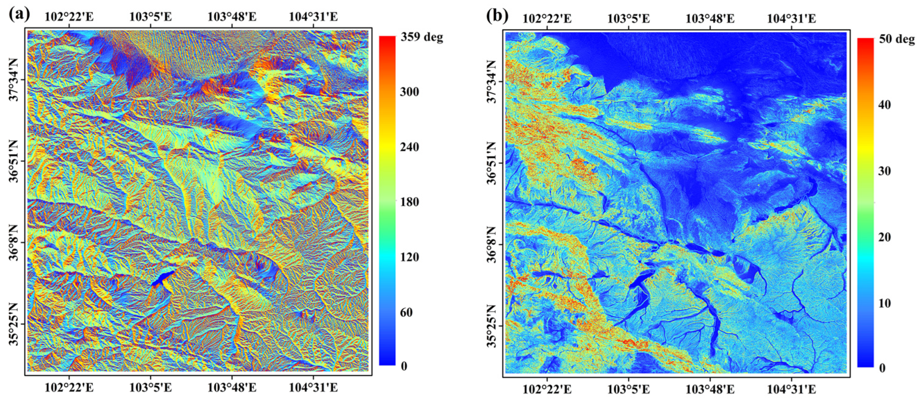
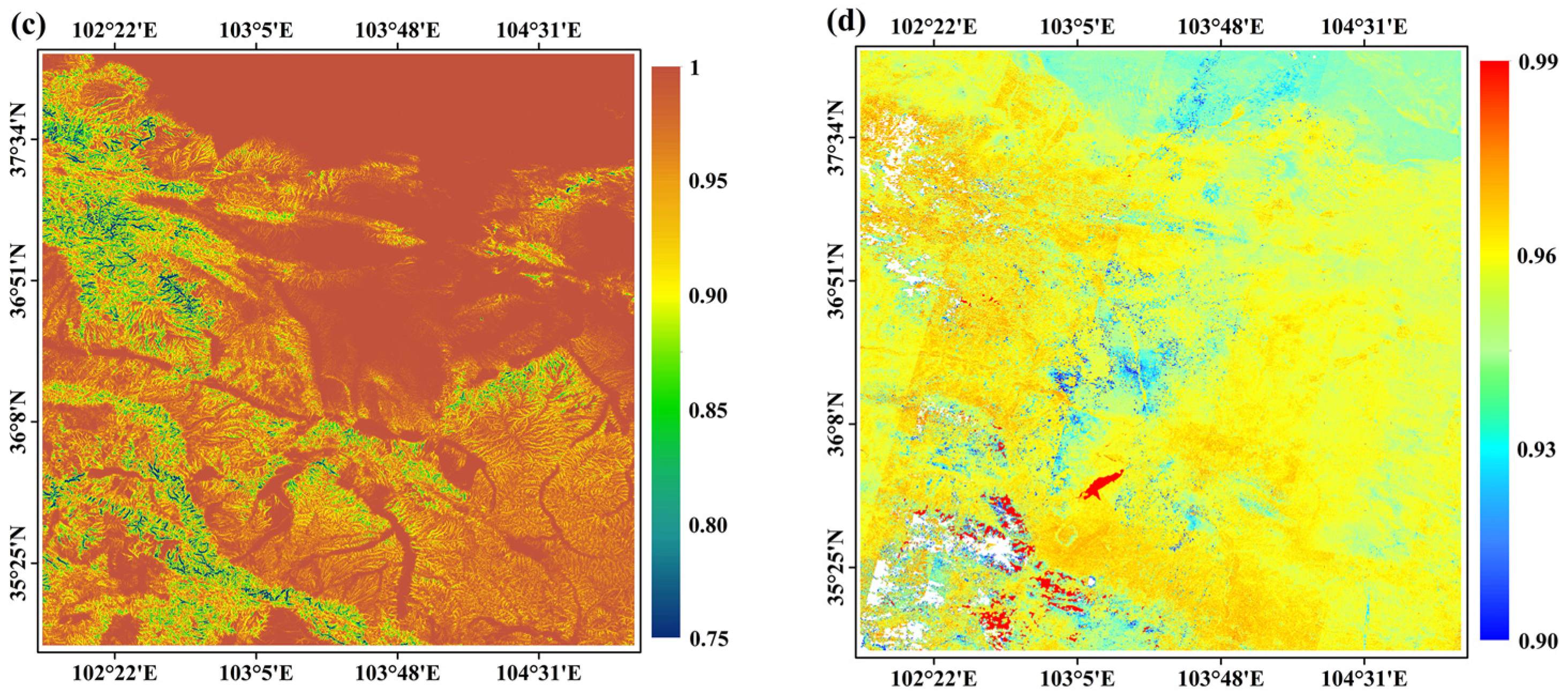
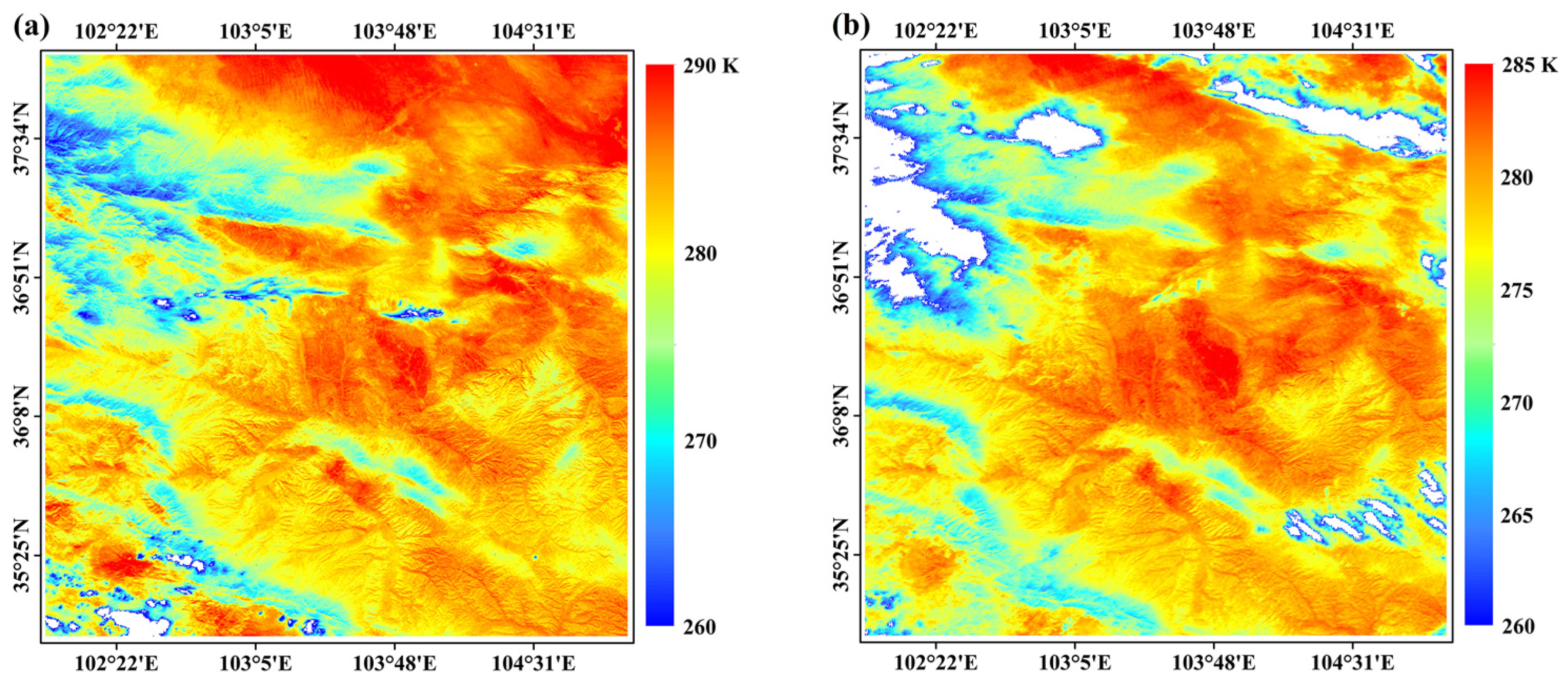
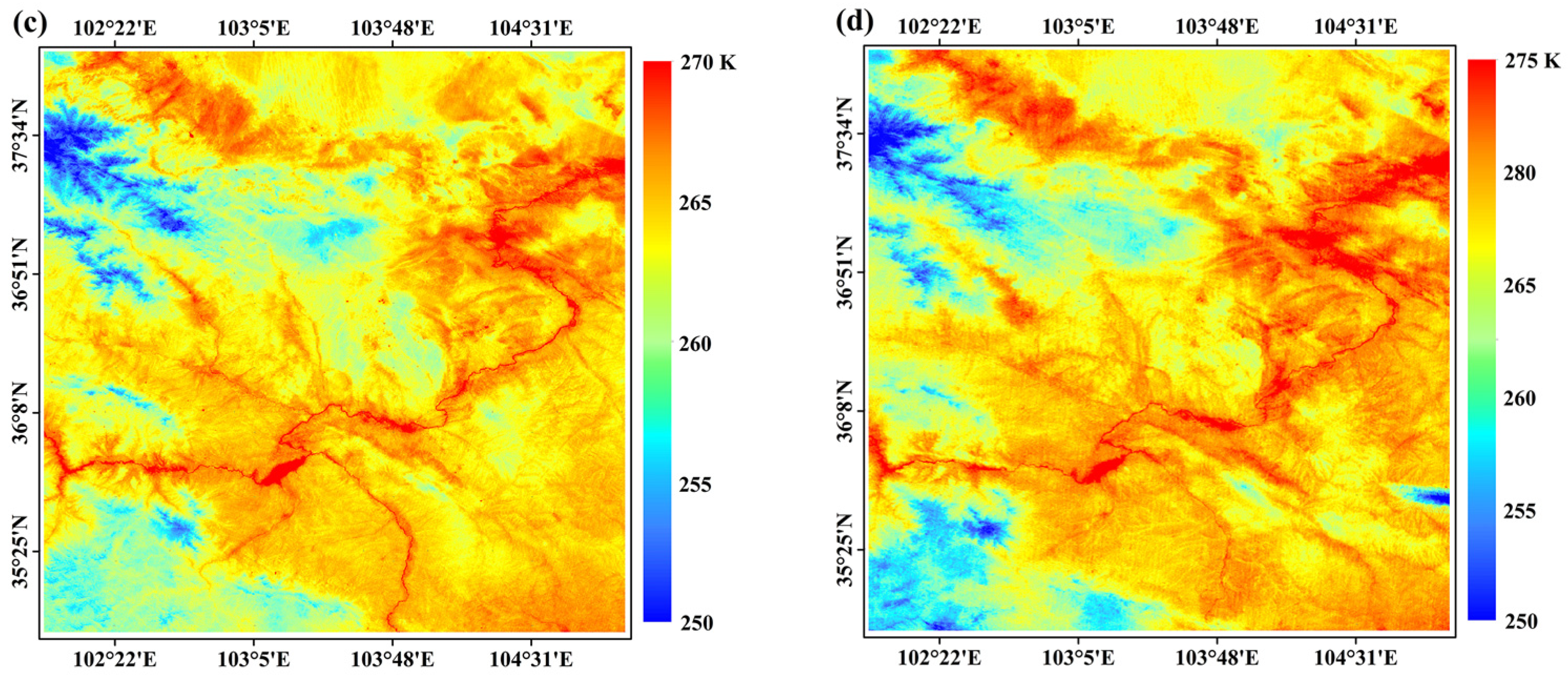
4.1. Application of the LST Retrieval Algorithm to Kunlun Mountain Images

Figure 3 shows the spatial extent of study area-I including (a) the aspect angle, (b) the slope angle, (c) the SVF, and (d) ASTER GED soil emissivity obtained from the NDVI threshold method. The slope angle values of the northeast part are close to 0°, and the area has an elevation of about 1200 m, which represents the lowest level in this region. Most flat surfaces are distributed in this area, with 0° aspect angle values. Mountains are predominantly located in the western region, and the smaller SVF values are located in this region. Meanwhile, the areas with larger slope angle values are consistent with the areas of smaller SVF values and various aspect angle values. The ASTER GED soil emissivity ranges from 0.90 to 0.99, and the emissivity distribution is around 0.96 in most regions. However, obvious banding effects and missing values exist in the ASTER GED products, which can cause significant errors in the LST retrieval. The white regions in Figure 3d represent missing values from the ASTER GED products. In the subsequent LST retrieval algorithm, these pixels are filled with the average values of the bare soil emissivity.

Figure 4 shows the spatial distribution of the retrieved LST images using FY-3D data in the Kunlun Mountains. In this study, four images with different UTC times are selected to retrieve the mountainous LST. Higher LSTs are found at lower altitudes, while LSTs below 260 K are found for higher altitude areas. The LST minimum occurs at the northwest area of the images, and has an elevation higher than 1400 m. In these regions, the higher slope angle areas are equivalent to the smaller SVF value areas in Figure 3b,c. There are cloudy pixels in the LST images at 05:45 UTC on 10 November and 05:25 UTC on 11 November, which are not considered in this study. The LST spatial distribution varies over time, and these images have similar distribution patterns at adjacent UTC times even with different dates. Retrieved images at 05:45 UTC and 05:25 UTC show similar trends in Figure 4a,b, and at 19:25 UTC and 18:30 UTC in Figure 4c,d there are similar LST distribution intervals. The LST ranges from 260 K to 290 K in Figure 4a,b, whereas the LST ranges from 250 K to 275 K in Figure 4c,d. In addition, the LST spatial distribution trend is continuous and reasonable in free-cloud pixels. White pixels are cloudy regions and are not considered in the retrieval process.

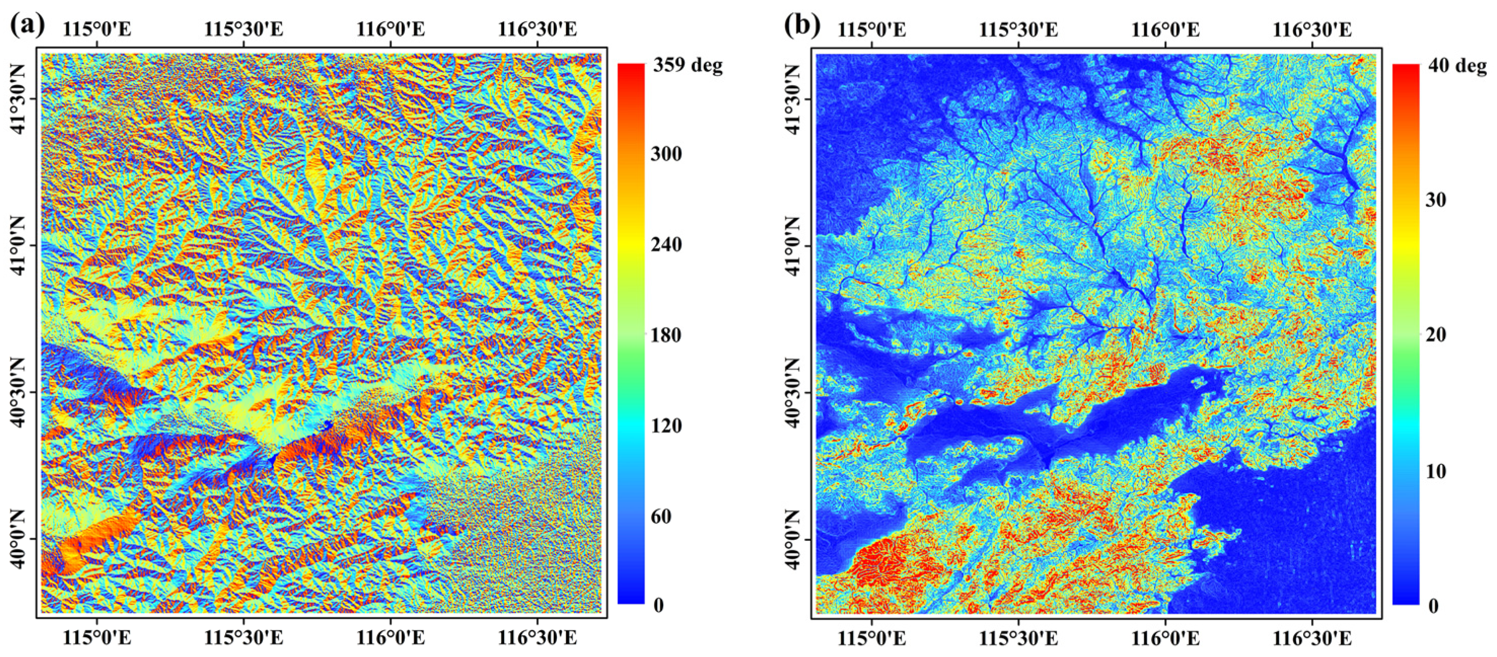
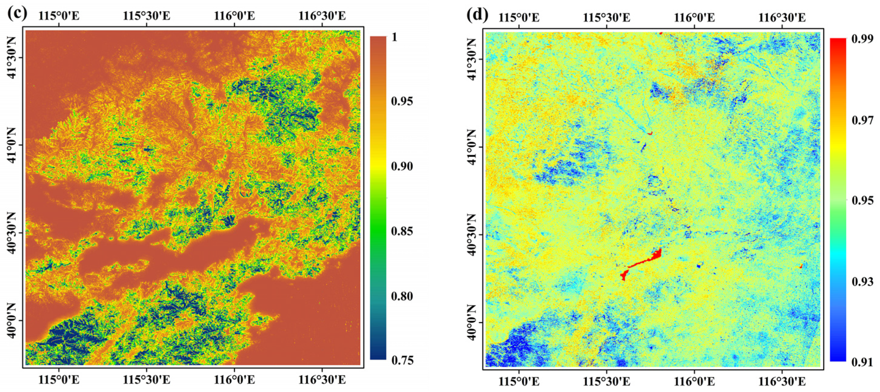
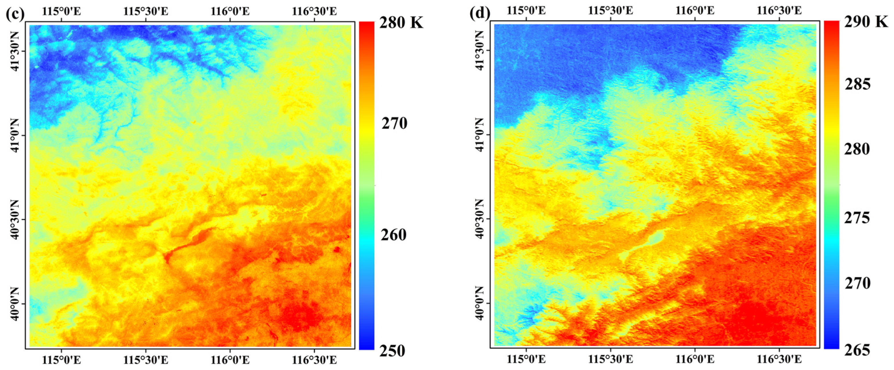
4.2. Application of the LST Retrieval Algorithm to Yanqing Zone Images

Figure 5 shows the spatial extent of the topographic factors including (a) the aspect angle, (b) the slope angle, (c) the SVF, and (d) ASTER GED soil emissivity in study area-II. The southeast direction of this region is the sea area, thus its topographic parameters are mostly similar to those of a flat surface whose slope angle and aspect angle both equal 0 and the SVF equals 1. The regions whose slope angle is close to 40° are mountainous areas, and it is obvious that the SVF is smaller than that of the sea-level regions. The higher slope angles correspond to areas with smaller SVF values. The mountainous ridges and valleys can be distinguished from the topographic parameter images when comparing with Figure 1b, whereas the ASTER GED soil emissivity image is slightly different, with an elevation trend.

Figure 6 shows the spatial distribution of the retrieved LST images, which are for four consecutive days with different UTC times. The spatial distribution of the LST images is similar to the elevation images in Figure 1b. The LST maximum occurs at the southeast corner of the study area, where the sea level has 0.99 surface emissivity. Meanwhile, the LST minimum occurs at the northwest corner of the study area, which covers a mountainous terrain with an elevation of 1400 m. In these regions, the slope angle, aspect angle, and SVF are equivalent to those of the homogeneous surfaces shown in Figure 6a–c. In addition, the LST spatial distributions in adjacent acquisition moments are similar to each other; see, for example, the images at 05:25 UTC in Figure 6a and 06:10 UTC in Figure 6d, 19:05 UTC in Figure 6b and 18:45 UTC in Figure 6c. They have the same distribution trends, whereas the obtained dates are different and the transit times are respectively 19:05 and 18:45 UTC. The LST ranges from 250 K to 280 K in Figure 6b,c, whereas the LST ranges from 260 K to 290 K in Figure 6a and 265 K to 290 K in Figure 6d. In addition, the LST spatial distribution trend is continuous and reasonable. Compared with an LST ranging from 250 K to 280 K, the spatial distribution of the LST images reaching 290 K is closer to the elevation distribution shown in Figure 1b.

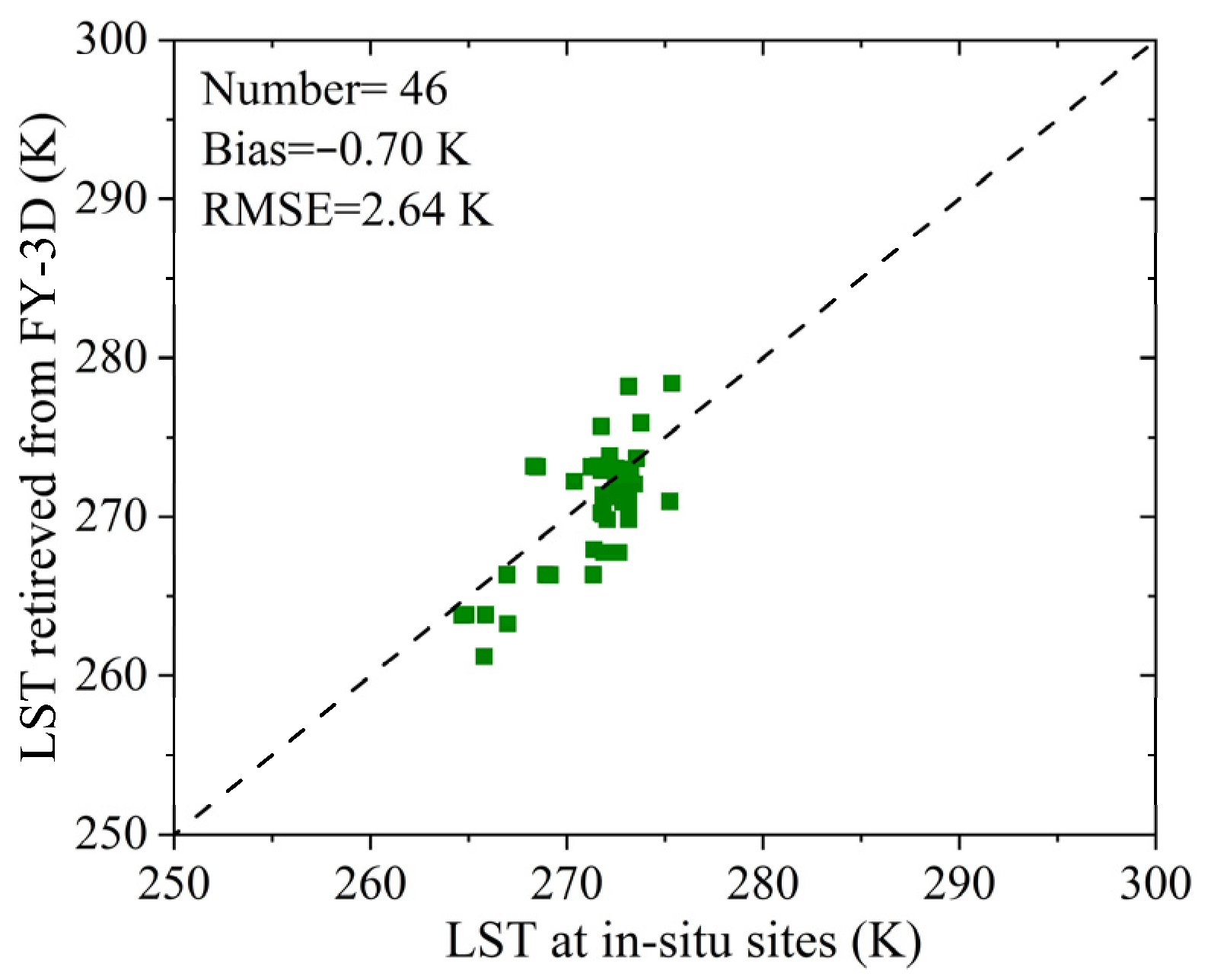
4.3. Accuracy Assessment of LST Using In Situ Measurements

The method adopted in this study used the iterative single-window algorithm using MRTE, which is proposed to correct for the terrain effect. The retrieved LST images are shown in Section 4.2, and a database of five in situ sites, which are shown in Figure 1c with data available from 1 November to 30 November 2021, was applied to validate the retrieved LST. Figure 7 shows the scatterplot of the LST comparison between the five in situ sites shown in Figure 1b and the retrieved FY-3D LST. The LST bias approximately is −0.70 K, whereas the LST RMSE is approximately 2.64 K for the five in situ sites. As shown in Figure 7, larger LST errors may be introduced by the geometric correction, cloud coverage, and strips of images. Due to missing data at the in situ sites, there are only several available data at sites A1703 and A1707. Although there are more data available at the other sites, the difficulty in obtaining the ground LST still hinders any subsequent analysis in this study. On the other hand, the retrieval LST varied over a wide range during November 2021, whereas the LST of the in situ sites was stable with varying snow coverage. The overall bias and RMSE between the retrieved LSTs and the five in situ stations are respectively −0.70 K and 2.64 K, and the LST retrieval algorithm performs better at the in situ sites A1701 and A1702 with the available cloud-free data.

5. Discussion and Conclusions

Section 4 demonstrates the retrieved LST images in Kunlun Mountain and the Yanqing Zone, which have different elevation differences. The elevation of the Kunlun Mountain ranges from 1200 m to 4800 m, whereas the elevation of the Yanqing Zone ranges from sea level to 2800 m. Two types of elevation differences are simultaneously used to retrieve the LST with different terrain structures. It represents the universalizability of single-window algorithms. However, there are some limitations to the LST retrieval algorithm. Firstly, the precision of the LSE and atmospheric parameters can directly affect the performance of single-window LST retrieval algorithms. It is important to select the correction methods for obtaining the LSE and atmospheric parameters. In this study, the NDVI threshold method relies on the ASTER GED emissivity products, which have problems with the strip effect and missing data values. A more accurate LSE product or estimation method is still necessary. On the other hand, the spatial resolution of the reanalysis data is lower and very different from the FY-3D MERSI-II data. Cloudy and rainy weather frequently occurs in mountainous areas, and they can also cause significant errors in the retrieval of the LST. Therefore, the influencing variables, including cloud coverage and strips of images, should be dealt with through a quantitative analysis and explanation in future research. Finally, in situ sites are an effective means of evaluating the performance of the retrieved LST, and more ground equipment should be engaged over mountainous areas in the future.

Mountainous surface temperature is the critical parameter in ecological, environmental, and climate monitoring research. In this study, the mountainous thermal infrared radiation transfer equation and an iterative single-channel algorithm are used to retrieve the LST over the mountainous areas of Kunlun Mountain and the Yanqing Zone. Correcting for the effect of the adjacent terrain, the retrieved LST results are summarized as follows:

To prove the generalizability of the MRTE and iterative single-window algorithm, terrain parameters including slope angle, aspect angle, and SVF were used to demonstrate the different topographic features of the two study areas. Although it is not consistent with their elevation differences, latitude, and longitude, they still have a common distribution of the LST. The slope angle maximum and the SVF minimum occur for mountainous valleys in both cases, whereas the LST minimum occurs at the mountainous ridges. The LST retrieval algorithm utilized in this study performs well in the Kunlun Mountain and the Yanqing Zone, whose spatial distribution is always smooth and reasonable with different satellite transit times.

Five in situ sites are also used to further demonstrate the accuracy and precision of the iterative single-window algorithm. The overall RMSE and bias between the in situ sites in the Yanqing Zone and retrieval from the FY-3D LST are respectively −0.70 K and 2.64 K. The LST retrieval algorithm performs better at in situ sites A1701 and A1702 with the available cloud-free data.

The topographic influences on the surface parameters are varied at different spatial resolutions [44], and the fine-resolution data should be improved and used to explore the topographic influences.

References

1. Anderson, M.; Norman, J.; Kustas, W.; Houborg, R.; Starks, P.; Agam, N. A thermal-based remote sensing technique for routine mapping of land-surface carbon, water and energy fluxes from field to regional scales. Remote Sens. Environ. 2008, 112, 4227–4241. [Google Scholar] [CrossRef]
2. Chen, J.; Liu, J. Evolution of evapotranspiration models using thermal and shortwave remote sensing data. Remote Sens. Environ. 2020, 237, 111594. [Google Scholar] [CrossRef]
3. Zhang, Y.; Peña-Arancibia, J.; McVicar, T.R.; Chiew, F.H.S.; Vaze, J.; Liu, C.; Lu, X.; Zheng, H.; Wang, Y.; Liu, Y.; et al. Multi-decadal trends in global terrestrial evapotranspiration and its components. Sci. Rep. 2016, 11, 19124. [Google Scholar] [CrossRef] [PubMed]
4. Hu, T.; Renzullo, L.; Van Dijk, A.I.J.M.; He, J.; Tian, S.; Xu, Z.; Zhou, J.; Liu, T.; Liu, Q. Monitoring agricultural drought in Australia using MTSAT-2 land surface temperature retrievals. Remote Sens. Environ. 2020, 236, 111419. [Google Scholar] [CrossRef]
5. Liu, Y.; Yu, X.; Dang, C.; Yue, H.; Wang, X.; Niu, H.; Zu, P.; Cao, M. A dryness index TSWDI based on land surface temperature, sun-induced chlorophyll fluorescence, and water balance. ISPRS J. Photogramm. Remote Sens. 2023, 202, 581–598. [Google Scholar] [CrossRef]
6. West, H.; Quinn, N.; Horswell, M. Remote sensing for drought monitoring & impact assessment: Progress, past challenges and future opportunities. Remote Sens. Environ. 2019, 232, 111291. [Google Scholar] [CrossRef]
7. Huang, X.; Wang, Y. Investigating the effects of 3D urban morphology on the surface urban heat island effect in urban functional zones by using high-resolution remote sensing data: A case study of Wuhan, Central China. ISPRS J. Photogramm. Remote Sens. 2019, 152, 119–131. [Google Scholar] [CrossRef]
8. Liu, Z.; Zhan, W.; Lai, J.; Bechtel, B.; Lee, X.; Hong, F.; Li, L.; Huang, F.; Li, J. Taxonomy of seasonal and diurnal clear-sky climatology of surface urban heat island dynamics across global cities. ISPRS J. Photogramm. Remote Sens. 2022, 187, 14–33. [Google Scholar] [CrossRef]
9. Sobrino, J.A.; Oltra-Carrió, R.; Sòria, G.; Bianchi, R.; Paganini, M. Impact of spatial resolution and satellite overpass time on evaluation of the surface urban heat island effects. Remote Sens. Environ. 2012, 117, 50–56. [Google Scholar] [CrossRef]
10. Zhou, D.; Xiao, J.; Bonafoni, S.; Berger, C.; Deilami, K.; Zhou, Y.; Frolking, S.; Yao, R.; Qiao, Z.; Sobrino, J.A. Satellite remote sensing of surface urban heat islands: Progress, challenges, and perspectives. Remote Sens. 2019, 11, 48. [Google Scholar] [CrossRef]
11. Hansen, J.; Ruedy, R.; Sato, M.; Lo, K. Global surface temperature change. Rev. Geophys. 2010, 48, RG4004. [Google Scholar] [CrossRef]
12. Plummer, S.; Lecomte, P.; Doherty, M. The ESA Climate Change Initiative (CCI): A European contribution to the generation of the Global Climate Observing System. Remote Sens. Environ. 2017, 203, 2–8. [Google Scholar] [CrossRef]
13. Zheng, L.; Li, D.; Xu, J.; Xia, Z.; Hao, H.; Chen, Z. A twenty-years remote sensing study reveals changes to alpine pastures under asymmetric climate warming. ISPRS J. Photogramm. Remote Sens. 2022, 190, 69–78. [Google Scholar] [CrossRef]
14. Li, Z.-L.; Tang, B.-H.; Wu, H.; Ren, H.; Yan, G.; Wan, Z.; Trigo, I.F.; Sobrino, J.A. Satellite-derived land surface temperature: Current status and perspectives. Remote Sens. Environ. 2013, 131, 14–37. [Google Scholar] [CrossRef]
15. Li, Z.-L.; Wu, H.; Duan, S.-B.; Zhao, W.; Ren, H.Z.; Liu, X.; Leng, P.; Tang, R.; Ye, X.; Zhu, J.; et al. Satellite remote sensing of global land surface temperature: Definition, methods, products, and applications. Rev. Geophys. 2022, 61, e2022RG000777. [Google Scholar] [CrossRef]
16. Wu, Y.; Wang, N.; Li, Z.; Chen, A.; Guo, Z.; Qie, Y. The effect of thermal radiation from surrounding terrain on glacier surface temperatures retrieved from remote sensing data: A case study from Qiyi Glacier, China. Remote Sens. Environ. 2019, 231, 111267. [Google Scholar] [CrossRef]
17. Kapos, V.; Rhind, J.; Edwards, M.; Price, M.; Ravilious, C. Developing a map of the world’s mountain forests. In Forests in Sustainable Mountain Development: A State of Knowledge Report for 2000. Task Force on Forests in Sustainable Mountain Development; Cabi Publishing: Wallingford, UK, 2000; pp. 4–19. [Google Scholar] [CrossRef]
18. Wu, Y.; Wang, N.; He, J.; Jiang, X. Estimating mountainous glacier surface temperatures from Landsat-ETM+ thermal infrared data: A case study of Qiyi glacier, China. Remote Sens. Environ. 2015, 163, 286–295. [Google Scholar] [CrossRef]
19. Li, A.; Bian, J.; Zhang, Z.; Zhao, W.; Yin, G. Progresses, opportunities, and challenges of mountain remote sensing research. Natl. Remote Sens. Bull. 2016, 20, 1199–1215. [Google Scholar] [CrossRef]
20. Sandmeier, S.; Itten, K. A physically-based model to correct atmospheric and illumination effects in optical satellite data of rugged terrain. IEEE Trans. Geosci. Remote Sens. 1997, 35, 708–717. [Google Scholar] [CrossRef]
21. Sirguey, P. Simple correction of multiple reflection effects in rugged terrain. Int. J. Remote Sens. 2009, 30, 1075–1081. [Google Scholar] [CrossRef]
22. Lenot, X.; Achard, V.; Poutier, L. SIERRA: A new approach to atmospheric and topographic corrections for hyperspectral imagery. Remote Sens. Environ. 2009, 113, 1664–1677. [Google Scholar] [CrossRef]
23. Wu, S.; Wen, J.; You, D.; Hao, D.; Lin, X.; Xiao, Q.; Liu, Q.; Gastellu-Etchegorry, J. Characterization of remote sensing albedo over sloped surfaces based on DART simulations and in situ observations. J. Geophys. Res. Atmos. 2018, 123, 8599–8622. [Google Scholar] [CrossRef]
24. Bellasio, R.; Maffeis, G.; Scire, J.S.; Longoni, M.G.; Bianconi, R.; Quaranta, N. Algorithms to account for topographic shading effects and surface temperature dependence on terrain elevation in diagnostic meteorological models. Bound.-Layer Meteorol. 2005, 114, 595–614. [Google Scholar] [CrossRef]
25. Zhao, W.; Li, A. A review on land surface processes modeling over complex terrain. Adv. Meteorol. 2015, 2015, 607181. [Google Scholar] [CrossRef]
26. Wang, T.; Yan, G.; Mu, X.; Jiao, Z.; Chen, L.; Chu, Q. Toward operational shortwave radiation modeling and retrieval over rugged terrain. Remote Sens. Environ. 2018, 205, 419–433. [Google Scholar] [CrossRef]
27. Yan, G.; Wang, T.; Jiao, Z.; Mu, X.; Zhao, J.; Chen, L. Topographic radiation modeling and spatial scaling of clear-sky land surface longwave radiation over rugged terrain. Remote Sens. Environ. 2016, 172, 15–27. [Google Scholar] [CrossRef]
28. Yan, G.; Tong, Y.; Yan, K.; Mu, X.; Chu, Q.; Zhou, Y.; Liu, Y.; Qi, J.; Li, L.; Zeng, Y.; et al. Temporal extrapolation of daily downward shortwave radiation over cloud-free rugged terrains. Part 1: Analysis of topographic effects. IEEE Trans. Geosci. Remote Sens. 2018, 56, 6375–6393. [Google Scholar] [CrossRef]
29. Jiao, Z.; Yan, G.; Wang, T.; Mu, X.; Zhao, J. Modeling of land surface thermal anisotropy based on directional and equivalent brightness temperatures over complex terrain. IEEE J. Sel. Top. Appl. Earth Obs. Remote Sens. 2019, 12, 410–423. [Google Scholar] [CrossRef]
30. Hais, M.; Kučera, T. The influence of topography on the forest surface temperature retrieved from Landsat TM, ETM+ and ASTER. ISPRS J. Photogramm. Remote Sens. 2009, 64, 585–591. [Google Scholar] [CrossRef]
31. Lipton, A.E. Effects of slope and aspect variations on satellite surface temperature retrievals and mesoscale analysis in mountainous terrain. J. Appl. Meteorol. Climatol. 1992, 31, 255–264. [Google Scholar] [CrossRef]
32. Lipton, A.E.; Ward, J.M. Satellite-view biases in retrieved surface temperatures in mountain areas. Remote Sens. Environ. 1997, 60, 92–100. [Google Scholar] [CrossRef]
33. Zhu, X.; Duan, S.-B.; Li, Z.-L.; Zhao, W.; Wu, H.; Leng, P.; Gao, M.; Zhou, X. Retrieval of land surface temperature with topographic effect correction from Landsat 8 thermal infrared data in mountainous areas. IEEE Trans. Geosci. Remote Sens. 2021, 59, 6674–6687. [Google Scholar] [CrossRef]
34. Malbéteau, Y.; Merlin, O.; Gascoin, S.; Gastellu, J.; Mattar, C.; Olivera-Guerra, L.; Khabba, S.; Jarlan, L. Normalizing land surface temperature data for elevation and illumination effects in mountainous areas: A case study using ASTER data over a steep-sided valley in Morocco. Remote Sens. Environ. 2017, 189, 25–39. [Google Scholar] [CrossRef]
35. Weng, Q.; Firozjaei, M.; Kiavarz, M.; Alavipanah, S.; Hamzeh, S. Normalizing land surface temperature for environmental parameters in mountainous and urban areas of a cold semi-arid climate. Sci. Total Environ. 2019, 650, 515–529. [Google Scholar] [CrossRef]
36. Zhao, W.; Duan, S.-B.; Li, A.; Yin, G. A practical method for reducing terrain effect on land surface temperature using random forest regression. Remote Sens. Environ. 2019, 221, 635–649. [Google Scholar] [CrossRef]
37. Eom, H.-S.; Myoung-Seok, S. Seasonal and diurnal variations of stability indices and environmental parameters using NCEP FNL data over East Asia. Asia-Pac. J. Atmos. Sci. 2011, 47, 181–192. [Google Scholar] [CrossRef]
38. Hulley, G.C.; Hook, S.J.; Baldridge, A.M. Validation of the North American ASTER land surface emissivity database (NAALSED) version 2.0 using pseudo-invariant sand dune sites. Remote Sens. Environ. 2009, 113, 2224–2233. [Google Scholar] [CrossRef]
39. Hulley, G.C.; Hook, S.J.; Abbott, E.; Malakar, M.; Islam, T.; Abrams, M. The ASTER Global Emissivity Dataset (ASTER GED): Mapping Earth’s emissivity at 100 meter spatial scale. Geophys. Res. Lett. 2015, 42, 7966–7976. [Google Scholar] [CrossRef]
40. Horn, B. Hill shading and reflectance map. Proc. IEEE 1981, 69, 14–47. [Google Scholar] [CrossRef]
41. Dozier, J.; Frew, J. Rapid calculation of terrain parameters for radiation modeling from digital elevation data. IEEE Trans. Geosci. Remote Sens. 1990, 28, 963–969. [Google Scholar] [CrossRef]
42. Proy, C.; Tanré, D.; Deschamps, P.Y. Evaluation of topographic effects in remotely sensed data. Remote Sens. Environ. 1989, 30, 21–32. [Google Scholar] [CrossRef]
43. Duan, S.-B.; Li, Z.-L.; Wang, C.; Zhang, S.; Tang, B.-H.; Leng, P.; Gao, M.-F. Land-surface temperature retrieval from Landsat-8 single-channel thermal infrared data in combination with NCEP reanalysis data and ASTER GED product. Int. J. Remote Sens. 2019, 40, 1763–1778. [Google Scholar] [CrossRef]
44. Shi, H.; Xiao, Z. Exploring topographic effects on surface parameters over rugged terrains at various spatial scales. IEEE Trans. Geosci. Remote Sens. 2022, 60, 1–16. [Google Scholar] [CrossRef]
Figure 1. The location and elevation of the study areas. The overall regions of the FY-3D LST retrieved images of study area-I (a) and study area-II (b), and (c) the locations of the in situ stations.
Remotesensing 15 05465 g001
Figure 2. Spectral response functions in FY-3D bands 24 and 25.
Remotesensing 15 05465 g002
Figure 3. Spatial distribution of the study area-I (a) aspect angle, (b) slope angle, (c) SVF, and (d) ASTER GED bare soil emissivity, where the white regions represent missing values.
Remotesensing 15 05465 g003aRemotesensing 15 05465 g003b
Figure 4. Spatial distribution of retrieved LST images from FY-3D band 24 with the terrain correction effect on (a) 10 November (05:45 UTC time), (b) 11 November (05:25 UTC time), (c) 11 November (19:25 UTC time), and (d) 14 November (18:30 UTC time) in 2021.
Remotesensing 15 05465 g004aRemotesensing 15 05465 g004b
Figure 5. Spatial distribution of the study area-II (a) aspect angle, (b) slope angle, (c) SVF, and (d) ASTER GED bare soil emissivity.
Remotesensing 15 05465 g005aRemotesensing 15 05465 g005b
Figure 6. Spatial distribution of the retrieved LST images from FY-3D band 24 with the terrain correction effect on (a) 11 November (05:25 UTC time), (b) 12 November (19:05 UTC time), (c) 13 November (18:45 UTC time), and (d) 14 November (06:10 UTC time) in 2021.
Remotesensing 15 05465 g006aRemotesensing 15 05465 g006b
Figure 7. The scatterplot of the LST bias and RMSE between the five in situ sites (A1701, A1702, A1703, A1707, and A1708) and the retrieved FY-3D LST.
Remotesensing 15 05465 g007
Disclaimer/Publisher’s Note: The statements, opinions and data contained in all publications are solely those of the individual author(s) and contributor(s) and not of MDPI and/or the editor(s). MDPI and/or the editor(s) disclaim responsibility for any injury to people or property resulting from any ideas, methods, instructions or products referred to in the content.