Technical Note

A Satellite Observational Study of Topographical Effects on Daytime Shallow Convective Clouds

1
Key Laboratory for Humid Subtropical Eco-Geographical Processes of the Ministry of Education, Fujian Normal University, Fuzhou 350007, China
2
School of Geographical Sciences, Fujian Normal University, Fuzhou 350007, China
3
Department of Geography and Planning, University of Toronto, Toronto, ON M5S 3G3, Canada
4
School of Geography and Tourism, Shaanxi Normal University, Xi’an 710119, China
*
Author to whom correspondence should be addressed.
Remote Sens. 2023, 15(23), 5542; https://doi.org/10.3390/rs15235542
Submission received: 11 October 2023 / Revised: 16 November 2023 / Accepted: 26 November 2023 / Published: 28 November 2023
(This article belongs to the Special Issue Remote Sensing of Aerosols, Planetary Boundary Layer, and Clouds)

Abstract

:
Shallow convective clouds (SCCs) frequently occur over mountainous terrain. However, previous studies have mostly focused on SCCs over flat surfaces. Here, the effects of mountainous terrains on the cloud size distributions (CSDs) and spatial distributions of SCCs are investigated using data obtained from the Landsat-8 satellite. We find that the CSDs are well-described by double power laws separated by scale breaks. The CSDs are controlled by two parameters, i.e., the scale breaks and the number of clouds with sizes between 0.2 and 1 times the scale breaks. We also find that the number of clouds generally increases with the elevation. In particular, the number of clouds larger than the scale breaks increases faster than that of the smaller clouds. The sizes of the larger clouds (the 90th and 95th percentiles) increase with the elevation, while the sizes of the smaller clouds are not sensitive to the elevation. It is suggested that the variations of cloud numbers and sizes with elevation should be used together with the CSDs to describe the cloud fields over mountainous terrains.

1. Introduction

Shallow convective clouds (SCCs) frequently appear both over the ocean [1] and over land [2,3,4], and play important roles in the earth system [5,6]. SCCs strongly reflect solar radiation, exerting a negative radiative forcing on the surface [7]. They can also transport pollutants and other substances from the boundary layer into the free troposphere [8]. Particularly, when SCCs transport vapor into the free troposphere, they can promote the development of deep convective clouds [9].
The typical sizes of SCCs are on the order of 102 m, which are much smaller than the typical grid intervals of global climate models [10] and global weather forecasting models [11]. Therefore, the effects of SCCs can only be considered via parameterization schemes. Many parameterization schemes of SCCs assume a single bulk updraft [12]. In this situation, all SCCs are assumed to have the same size. However, some studies have pointed out that these parameterization schemes cannot correctly treat the coupling between the cloud layer and the sub-cloud layer [13]. Other parameterization schemes that consider multiple bulk updrafts were therefore proposed [13,14,15]. In this type of parameterization schemes, the sizes of SCCs are assumed to follow prescribed distributions [14].
Cloud size is an important parameter describing SCCs. When a cloud develops upward, it entrains dry air from the environment into the cloud [16]. This decreases the liquid water content, and can potentially lead to cloud dissipation. Many studies have shown that the entrainment rate is inversely proportional to the cloud size [17,18]. In other words, a larger cloud is more resistant to the detrimental effect of entrainment. Therefore, a larger cloud possesses more positive vertical velocity, and can be more efficient in transporting substances into the free troposphere.
Cloud size distributions (CSDs) have been frequently reported in the literature. Plank [19] used photographs taken from high-flying aircrafts and found that the CSD follows an exponential distribution. Neggers et al. [20] used data obtained from the Landsat-5 satellite and found that the CSD follows a power law from the lower end up to a certain size. This result is also supported by results from large-eddy simulations [20,21]. Mieslinger et al. [22] used 1158 images obtained from the Advanced Spaceborn Thermal Emission and Reflection Radiometer (ASTER) satellite, and found that for SCCs larger than the scale break, the CSD can also be described by a power law, but with a different exponent. Stevens [23] suggested that the scale break is a controlling parameter of the CSD. It is worth mentioning that all CSDs mentioned above were obtained either over relatively flat land [19,20] or over the ocean [21,22].
It is well known that topography has substantial impacts on the development of SCCs [24,25]. In the daytime, solar radiation heats the slopes. Thereby, the air in contact with the slopes becomes warmer than the air far away from the slopes. The resulting horizontal temperature gradient leads to the formation of upslope winds [26]. If the air is sufficiently humid, clouds are produced when the upslope winds meet near the tops of the mountains. Both observational studies [27,28,29] and modelling studies [30,31] confirm that clouds prefer to develop near mountain tops. Note that these studies are mostly concerned with deep convective clouds instead of SCCs.
Rotach et al. [32] pointed out that more than 50% of the land surface is covered by hills and mountains. However, to the best of our knowledge, few studies have investigated the topographic effects on SCCs. In this study, we use data obtained from Landsat-8 to investigate whether the presence of topography affects the CSDs of SCCs. Furthermore, since CSDs are defined for a cloud field over a large area (on the order of 102 to 104 km2), it does not describe the spatial distribution of SCCs. Therefore, we also investigate how the sizes of SCCs vary with the elevation.
In Section 2, we present the methods. Section 3 first presents the CSDs, and then the variations of cloud sizes and cloud numbers with the elevation. A discussion is presented in Section 3.3. Section 4 summaries this study, and then provides perspectives for future studies.

2. Study Area, Data, and Methods

2.1. Study Area

This study focuses on SCCs in Southeast China (Figure 1). Due to the warm and humid climate, SCCs frequently occur in this area [2]. According to Warren et al. [3], the frequency of occurrence of SCCs is 23% in summer (June, July, and August), and is over 10% in spring (March, April, and May) and autumn (September, October, and November). The study area is characterized by mountainous terrain, with the minimum and maximum elevations of −70 m and 3838 m, respectively, and the mean elevation of 283 m. Such a complex topographic condition is suitable for the study of topographic effects on SCCs.

2.2. Data

The Advanced Spaceborne Thermal Emission and Reflection Radiometer (ASTER) Global Digital Elevation Model version 2 (GDEMV2) is used in this study. It has a resolution of 30 m and is freely available (https://www.jspacesystems.or.jp/ersdac/GDEM/E/index.html (accessed on 9 September 2023)). Compared to GDEMV1, the vertical accuracy of GDEMV2 has been improved from ± 20 m to ± 17 m. For regions that are predominantly mountainous or hilly, GDEMV2 is more reliable than the shuttle radar topography mission digital elevation model (SRTM DEM) product [33].
Cloud information was obtained from the Operational Land Imager (OLI) and Thermal Infrared Sensor (TIRS) onboard the Landsat-8 satellite. The Landsat-8 satellite crosses the equator at 10:00 am ± 15 min local time, and has a revisit period of 16 days. To the best of our knowledge, no method is currently available to automatically identify Landsat-8 scenes that are dominated by SCCs. Therefore, we selected scenes by eye inspection, and 114 scenes were obtained. The scenes span the period from 2014 to 2023.
Each Landsat-8 scene covers a spatial area of approximately 190 km × 190 km. Due to the spatial variations of weather conditions, it is unusual that such a large area is covered by a single cloud type, e.g., a SCC. As a result, the scenes need to be cropped to exclude cloud types other than SCCs. For clarity, the remaining scenes after cropping are called samples. Two constraints were imposed during the cropping. First, the samples are rectangular, and the four edges are parallel to the original Landsat-8 scenes. Second, each edge of the samples is longer than 70 km. This length is big enough to cover a sufficient number of SCCs. More importantly, it is close to the grid interval of global climate models, so our results can be used in the parameterization of SCCs. For each of the 114 scenes, at least one and at most four samples were obtained after cropping. A total of 292 samples were produced in total. Their positions are shown in Figure 1.

2.3. Cloud Identification Method

An official cloud mask product of Landsat-8 scenes is available. It uses the Fmask 4.0 algorithm [34] and has a high overall accuracy. However, it is found that the official product sometimes incorrectly identifies water bodies and riverbanks as clouds, and sometimes incorrectly identifies scattered SCCs as cloud decks when the SCCs develop in a cold air mass. These misidentifications cannot be ignored for the purpose of this study, so a revised algorithm was developed. The bands used in the revised algorithm are listed in Table 1.
Following Zhu et al. [35], potential cloudy pixels were first identified using the normalized difference vegetation index ( N D V I ), which is defined as
N D V I = B a n d 5 B a n d 4 B a n d 5 + B a n d 4
here, B a n d 4 and B a n d 5 are the top-of-atmosphere (TOA) reflectance of the fourth and fifth bands. For cloudy pixels, the N D V I is usually much smaller than 1. Here, we used a threshold value of 0.5. The reflectance of clouds is flat in the visible range, so clouds look white. The “whiteness” index is defined as [36]:
W h i t e n e s s = i = 2 4 | B a n d i -   M e a n V i s | / M e a n V i s
M e a n V i s = 1 3 i = 2 4 B a n d i
here, B a n d i is the TOA reflectance of the i -th band. The cloud is whiter when the whiteness index is closer to 0. Here, a threshold of 0.6 was used. The results of this step were still contaminated by water bodies, buildings, bare soils, etc.
Water has a small reflectance in the NIR band, so water bodies can be effectively removed using this band. A threshold value of 0.15 was selected. In addition, for buildings and bare soils, the reflectance of Band 6 is larger than that of Band 5 [37], while for clouds, the reflectance of Band 6 is smaller than that of Band 5, so another criterion was applied:
B a n d 6 < B a n d 5
Clouds are cooler than the surface. Zhu et al. [35] used a fixed threshold of brightness temperature (BT), derived from band 10. Here, a dynamic BT threshold was obtained for each sample using the Otsu algorithm, which categorizes the pixel-level BTs into two clusters so that a threshold BT is defined. Pixels with BTs lower than the threshold BT are identified as cloudy pixels.
After applying all the criteria discussed above, it was found that the results were still contaminated by noise pixels and elongated features (e.g., roads), and it was also found that some clouds are only briefly connected. These were avoided by performing morphological opening, which first erodes the pixels at the edge of the object, and then dilates the resulting object. Figure 2 shows an example of the cloud identification results. A comparison of Figure 2c,d indicates that the noise pixels were removed and the briefly connected clouds were separated, and a comparison of Figure 2b,e reveals that cities and roads were removed. Figure 2 suggests that the clouds were correctly identified.
Sixty samples were randomly selected to further evaluate the accuracy of the cloud identification results. For each sample, the cloud identification results produced by the aforementioned algorithm are compared with visual interpretation results at 100 randomly selected points. The mean producer’s accuracies are 87.3% for cloudy pixels and 99.5% for clear pixels. The mean user’s accuracies are 94.6% for cloudy pixels and 98.4% for clear pixels. The mean overall accuracy is 98.1% and the mean κ coefficient is 0.87. These metrics indicate that the cloud identification method is reliable.

3. Results and Discussion

3.1. Cloud Size Distribution

The identified cloudy pixels were four-way connected to form clusters. Each cluster is defined as a cloud [9]. The size of a cloud is defined as:
l = A ,
where A is the area of the cloud. The CSD is defined as:
N l = d N d l ,
where d N is the number of clouds whose sizes are between l and l + d l . In practice, bins of finite sizes were used to calculate the CSD, so that:
N l N l ,
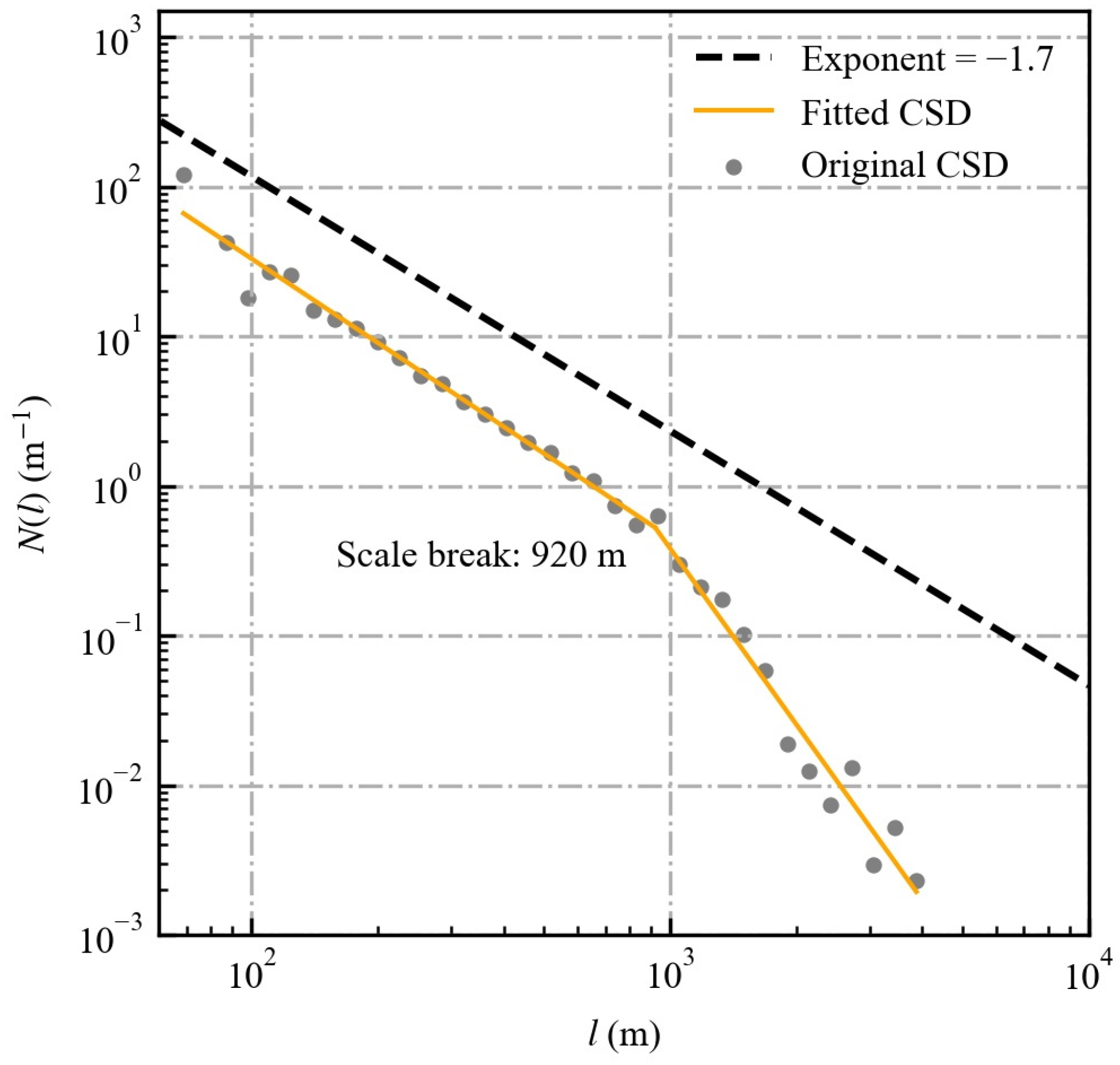
where N is the number of clouds in the size bin whose width is l . Two methods are frequently used to establish the size bins, i.e., linear binning and logarithmic binning. These two methods produce slightly different CSDs [22]. Here, we adopted the logarithmic binning. An example CSD is shown with the dots in Figure 3. Hereafter, the CSD calculated using Equation (7) is called the original CSD, so that it can be distinguished from the fitted CSD discussed below.
As discussed in Section 1, various functional forms have been proposed to describe CSDs. In this study, we adopted the power law because it fits the data well, as shown later. Specifically, the fitted CSD is described as:
N ( l ) = a 1 l b 1 ,                                               (   l < l S B ) a 2 l b 2 .                                               (   l l S B )
here, a 1 , b 1 , a 2 , and b 2 are constants, and l S B is the scale break. These five parameters are obtained using piecewise regression [38,39]. Note that logarithms are taken for both l and N ( l ) before the piecewise regression is invoked. The corresponding fitted CSD is also shown in Figure 3. It is clearly seen that the CSD follows two power laws separated by a scale break.
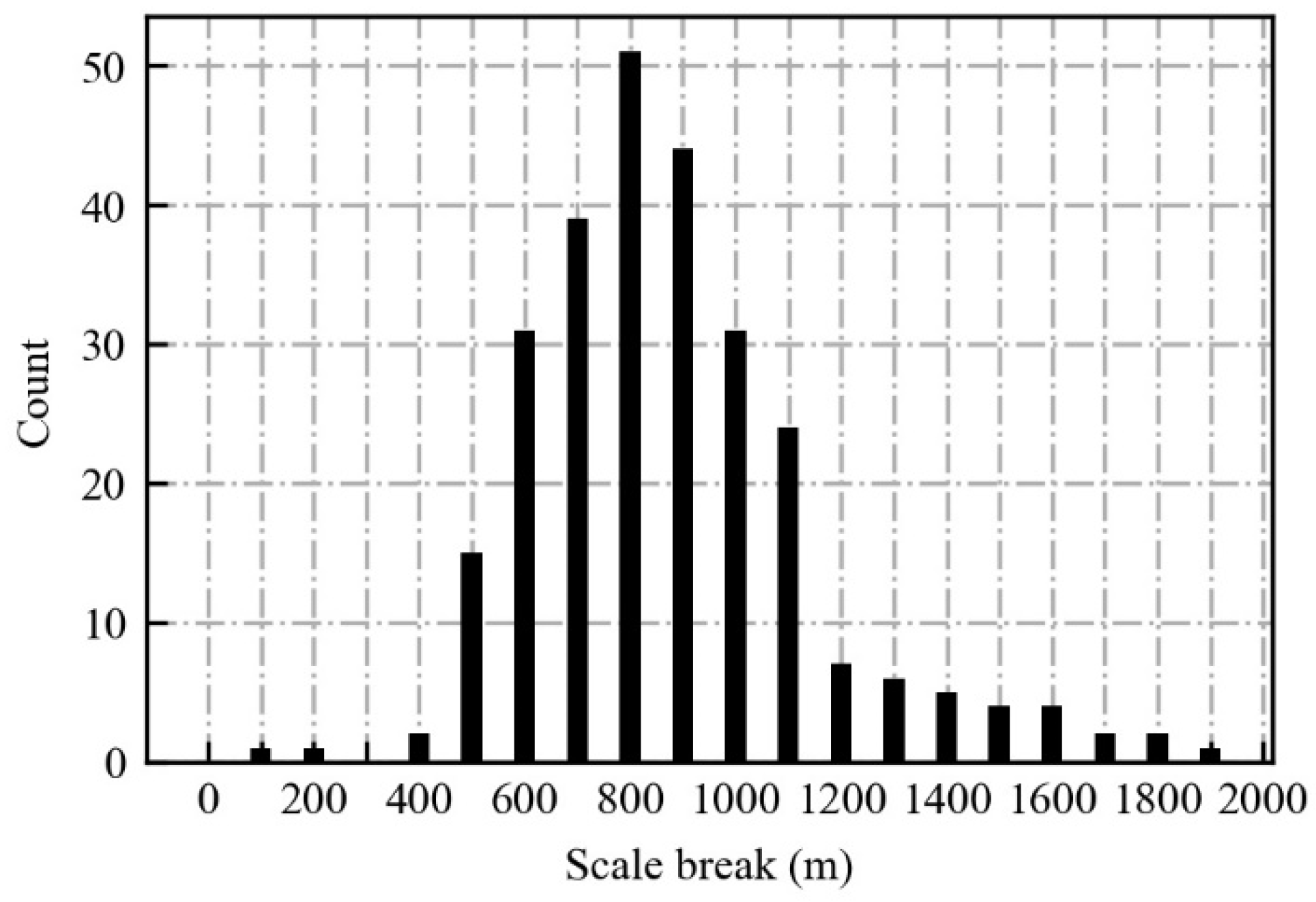
Piecewise regression was performed on each sample to derive the fitted CSDs and the associated scale breaks. We first focus on the scale breaks, as shown in Figure 4. The scale break varies from 100 to 1900 m. This is similar to the results of Neggers et al. [15], who found that the scale break varies from 400 to 1250 m. We note that the variation of scale break in this study is caused by the variation of surface properties (e.g., topography) and weather conditions, while the variation of scale break in Neggers et al. [15] is mainly caused by the diurnally varying surface heating. Figure 4 also shows that the scale break has a mode at 800 m. Further investigation is required to understand the formation of the mode.
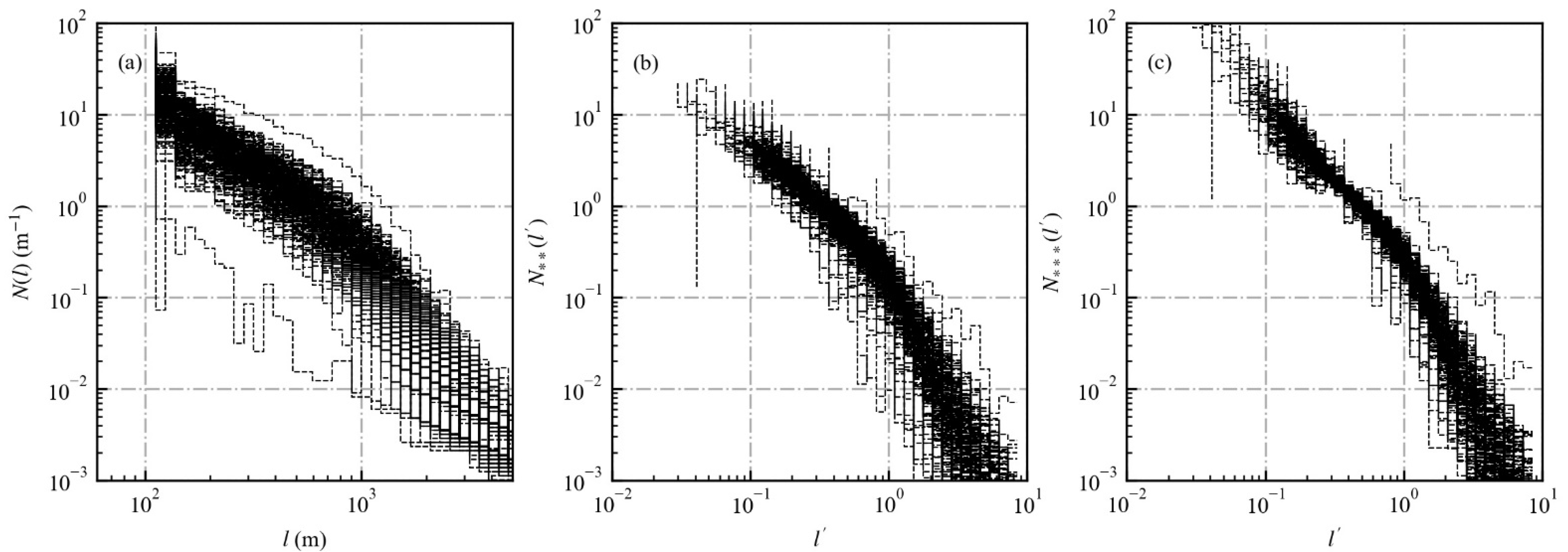
The original CSDs of all samples are shown in Figure 5a. Due to the variations of surface properties and weather conditions, the cloud number at a given cloud size varies by approximately one order of magnitude, and it is difficult to identify the power laws. In order to collapse the CSDs, Neggers et al. [15] normalized both the cloud size and the cloud number. Specifically, the normalized cloud size is defined as:
l = l l S B .
In this situation, the CSD becomes N l , and is related to N l via
N l = N l l S B
The cloud numbers are further normalized by the total number of clouds:
N 0 ~ = 0 N l d l .
Note that the subscript on the left-hand side is used to emphasize that clouds of all sizes are included. After the two normalizations, the CSD becomes
N l = N l N 0 ~
Figure 5b shows the normalized CSDs, as defined by Equation (12), for all samples. It is seen that the normalized CSDs clearly exhibit the double power laws, consistent with the findings of Neggers et al. [15]. However, Figure 5b also shows that even after the two normalizations, the normalized cloud number still varies by approximately an order of magnitude at a given cloud size.
For satellite data, the cloud size has a finite lower limit, which is related to the pixel size, so the lower limit of integration of Equation (11) is actually not 0, but is determined by the pixel size and the scale break. Furthermore, Figure 4 shows that the scale break varies substantially from one sample to another. In this situation, the lower limit of integration also varies substantially. This means that the integration is performed for substantially different intervals. Similar arguments also apply to the upper limit of integration. We note that the integration of Equation (11) is much more sensitive to the lower end than to the upper end due to the double-power law behavior of the CSD. In this study, we normalize the cloud numbers using
N 0.2 ~ 1 = 0.2 1 N l d l .
The CSD becomes:
N l = N l N 0.2 ~ 1 .
With the help of Equation (13), the interval of integration is explicitly controlled. Figure 5c shows the CSDs as defined by Equation (14). Obviously, the revised method of normalization collapses the data better.
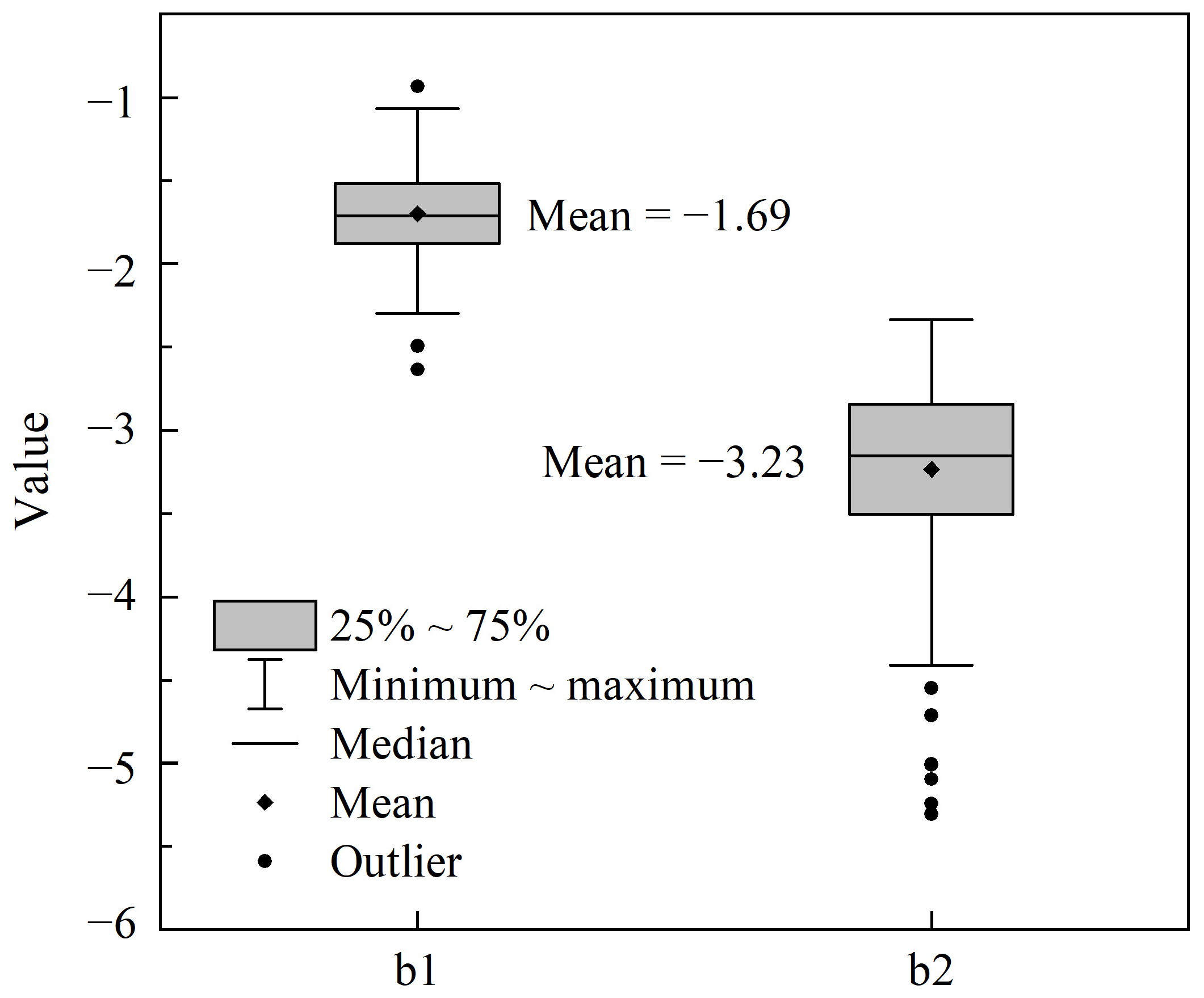
The values of b 1 and b 2 in Equation (8) are shown in Figure 6. The mean values of b 1 and b 2 are very close to their counterparts obtained by Mieslinger et al. [22], who investigated SCCs over oceans. Other studies usually reported values for b 1 but not for b 2 . The reported values of b 1 vary from −1.7 [15] to −1.9 [40] and −2.5 [41]. It is clear that these values of b 1 are within the range found by this study (Figure 6).

3.2. The Variation of Cloud Numbers and Sizes with the Elevation

By inspecting individual samples (e.g., Figure 2), it is clear that the presence of topography substantially affects the spatial distribution of SCCs. In order to quantitatively investigate how the number and sizes of clouds vary with the elevation, the connection between clouds and elevation needs to be established. This is simply carried out by defining the centroid of a cloud to be the position of the cloud [9,42], after which the elevation of the position right below the centroid of the cloud is connected to the cloud. In addition, since the samples cover different regions, the range of the elevation varies from one sample to another. In this situation, the elevation is normalized so that all samples can be averaged to produce an overall picture. The normalized elevation is defined as z n = z z 0 / z 1 z 0 , where z is the elevation, and z 0 and z 1 are the smallest and largest elevations associated with the sample.
The variation of the cloud number density with the elevation is shown in Figure 7. Six classes are defined according to the normalized cloud size. For each sample, the cloud number density of each size class is calculated for each elevation bin. Here, 10 equally-spaced bins of normalized elevation are used. As discussed above, the total number of clouds in each sample varies by approximately an order of magnitude. Thus, the cloud number densities are also normalized by N 0.2 ~ 1 before they are averaged over all the samples.
At a given elevation, Figure 7a shows that the cloud number density decreases with cloud size. This is consistent with the characteristics of the CSDs discussed in Section 3.1. For each size class, the cloud number density generally increases with the elevation. Furthermore, Figure 7b shows that the number density of the largest clouds (e.g., those with l > 1) increases faster than that of the smaller clouds. This indicates that the fraction of large clouds increases with the elevation. Near the higher end of the elevation, the variation of the cloud number density with the elevation becomes more complicated, e.g., the number density of clouds with 0 < l < 0.2 decreases with the elevation while the number density of clouds with 0.4 < l < 0.6 increases with the elevation. Further investigation is required to understand this complicated behavior.
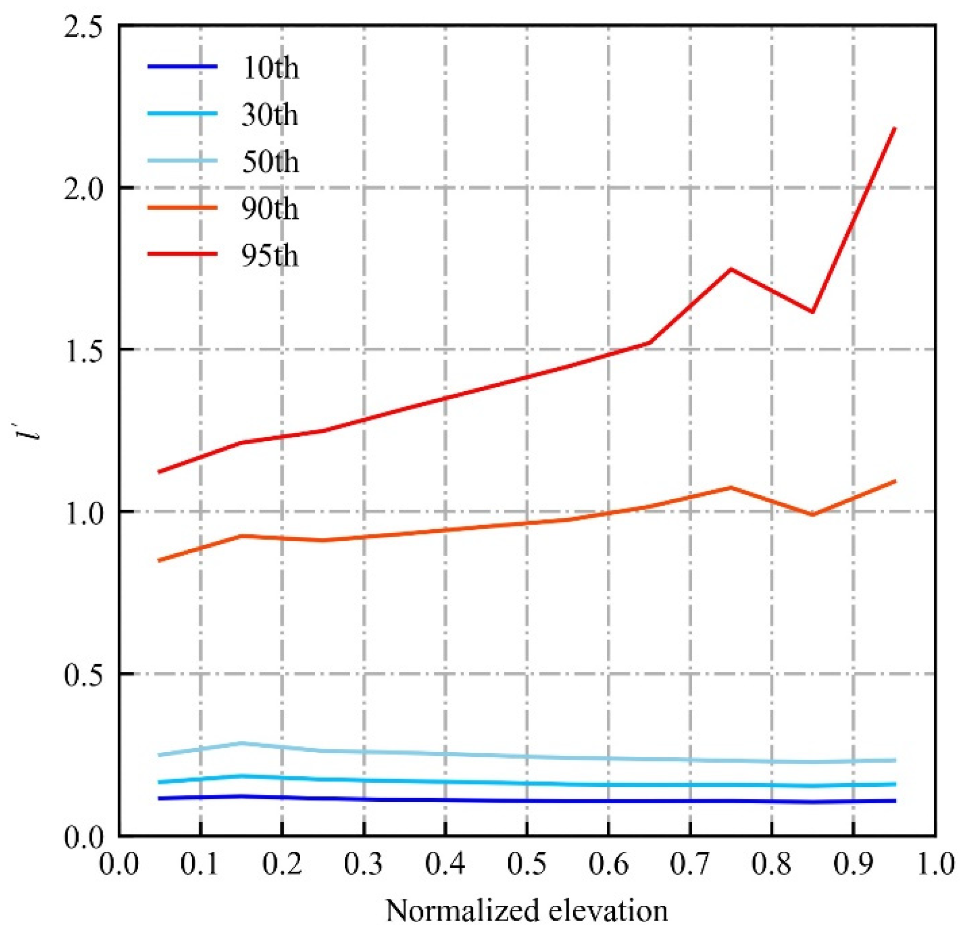
The variation of the cloud size with the elevation is shown in Figure 8. For small clouds, e.g., those at the 10th, 30th, and 50th percentiles, their sizes hardly change with the elevation. For large clouds, e.g., those at the 90th and 95th percentiles, their sizes increase with the elevation, and the size of the clouds at the 95th percentile increases faster than the size of the clouds at the 90th percentile. Previous studies have shown that larger SCCs are more likely to develop into deep convective clouds [9], and Figure 8 suggests that deep convective clouds tend to form near the top of the mountains. This is consistent with the results of previous studies [29,43].

3.3. Discussions

Section 3.1 shows that even in the presence of topography, CSDs can also be described by double power laws separated by scale breaks, similar to CSDs obtained over homogeneous surfaces. However, Section 3.2 shows that both the number and sizes of clouds do vary with the elevation. This indicates that it is not sufficient to describe cloud fields with CSDs only. The variations of cloud numbers and cloud sizes with the elevation, and probably some other information, should be used together with the CSDs to describe the cloud fields over mountainous terrains.

4. Conclusions

Shallow convective clouds (SCCs) frequently occur over mountainous terrain. However, few studies investigated topographic effects on SCCs. This study investigates the topographic effects on SCCs using scenes of the Landsat-8 satellite and an algorithm specifically designed for identifying SCCs.
We found that the cloud size distributions (CSDs) over mountainous terrains are well-described by double power laws separated by scale breaks, similar to the results obtained for SCCs over homogeneous surfaces, such as ocean surfaces. The CSDs are controlled by two parameters. The first is the scale break, and the second is the number of clouds with sizes between 0.2 and 1 times the scale breaks. The second parameter is different from that used by a previous study [15], where the number of all clouds is used. The number of clouds generally increases with the elevation, regardless of the sizes of the clouds. Furthermore, it was found that the number of clouds larger than the scale breaks increases faster than that of the smaller clouds. It was also found that the sizes of the clouds at the 90th and 95th percentiles increase with the elevation, while the sizes of the clouds at lower percentiles hardly vary with the elevation. These results indicate that large clouds tend to develop near the tops of the mountains. Our results suggest that cloud fields over mountainous terrains cannot be simply described with CSDs; other information, such as the variations of cloud numbers and cloud sizes with the elevation, should also be used.
Several aspects can be explored to further enhance our understanding of topographic effects on SCCs. First, more samples of SCCs should be collected. In this study, only 292 samples were used, so it is unclear whether the results of this study can be generalized to other regions. In order to obtain more samples, a larger study area and more satellites (e.g., other satellites of the Landsat series, ASTER, and the Sentinel series) should be utilized. However, as discussed earlier, no automatic method is currently available to select scenes dominated by SCCs, so it is difficult to increase the number of samples. We hope that the rapidly developing machine learning technique will provide a solution to accelerate the identification of SCCs from high-resolution satellite data. Second, the satellite data should be combined with meteorological data to investigate how the topographic effects on SCCs are modified by meteorological conditions, such as surface wind speed, boundary-layer height, atmospheric stability, and others. Special attention should be paid to how the scale break varies with these meteorological conditions, because the scale break is probably a controlling parameter of the CSD.

Author Contributions

Conceptualization, S.F.; methodology, G.X. and S.F.; software, G.X.; validation, G.X., S.F. and R.S.; formal analysis, G.X. and S.F.; investigation, G.X. and S.F.; resources, J.L.; data curation, G.X.; writing—original draft preparation, G.X. and S.F.; writing—review and editing, J.L. and R.S.; visualization, G.X. and Y.L.; supervision, S.F. and J.L.; project administration, J.L.; funding acquisition, S.F. All authors have read and agreed to the published version of the manuscript.

Funding

This research was funded by National Natural Science Foundation of China grant number 42105080, and Natural Science Foundation of Fujian Province grant number 2022J01643. And The APC was funded by 42105080.

Data Availability Statement

The data presented in this study are available on request from the corresponding author. The data are not publicly available due to privacy.

Acknowledgments

We thank Rong Wang and Yang Wang for helpful discussions. We thank the Landsat-8 team in NASA/USGS for sharing their data with the community.

Conflicts of Interest

The authors declare no conflict of interest.

References

  1. Warren, S.G.; Hahn, C.J.; London, J.; Chervin, R.M.; Jenne, R.L. Global Distribution of Total Cloud Cover and Cloud Type Amounts Ocean; NCAR Technical Notes; University Corporation for Atmospheric Research: Boulder, CO, USA, 1988. [Google Scholar]
  2. Dror, T.; Koren, I.; Altaratz, O.; Heiblum, R.H. On the Abundance and Common Properties of Continental, Organized Shallow (Green) Clouds. IEEE Trans. Geosci. Remote Sens. 2021, 59, 4570–4578. [Google Scholar] [CrossRef]
  3. Warren, S.G.; Hahn, C.J.; London, J.; Chervin, R.M.; Jenne, R.L. Global Distribution of Total Cloud Cover and Cloud Type Amounts Land; NCAR Technical Notes; University Corporation for Atmospheric Research: Boulder, CO, USA, 1986. [Google Scholar]
  4. Tian, J.; Zhang, Y.; Klein, S.A.; Wang, L.; Öktem, R.; Romps, D.M. Summertime Continental Shallow Cumulus Cloud Detection Using GOES-16 Satellite and Ground-Based Stereo Cameras at the DOE ARM Southern Great Plains Site. Remote Sens. 2021, 13, 2309. [Google Scholar] [CrossRef]
  5. Bony, S.; Stevens, B.; Frierson, D.M.W.; Jakob, C.; Kageyama, M.; Pincus, R.; Shepherd, T.G.; Sherwood, S.C.; Siebesma, A.P.; Sobel, A.H.; et al. Clouds, circulation and climate sensitivity. Nat. Geosci. 2015, 8, 261–268. [Google Scholar] [CrossRef]
  6. Fast, J.D.; Berg, L.K.; Alexander, L.; Bell, D.; D’Ambro, E.; Hubbe, J.; Kuang, C.; Liu, J.; Long, C.; Matthews, A.; et al. Overview of the HI-SCALE Field Campaign: A New Perspective on Shallow Convective Clouds. Bull. Am. Meteorol. Soc. 2019, 100, 821–840. [Google Scholar] [CrossRef]
  7. Berg, L.K.; Kassianov, E.I.; Long, C.N.; Mills, D.L. Surface summertime radiative forcing by shallow cumuli at the Atmospheric Radiation Measurement Southern Great Plains site. J. Geophys. Res. 2011, 116, D01202. [Google Scholar] [CrossRef]
  8. Chen, G.; Xue, H.; Feingold, G.; Zhou, X. Vertical transport of pollutants by shallow cumuli from large eddy simulations. Atmos. Chem. Phys. 2012, 12, 11319–11327. [Google Scholar] [CrossRef]
  9. Fu, S.; Rotunno, R.; Chen, J.; Deng, X.; Xue, H. A large-eddy simulation study of deep-convection initiation through the collision of two sea-breeze fronts. Atmos. Chem. Phys. 2021, 21, 9289–9308. [Google Scholar] [CrossRef]
  10. Richter, I.; Tokinaga, H. An overview of the performance of CMIP6 models in the tropical Atlantic: Mean state, variability, and remote impacts. Clim. Dyn. 2020, 55, 2579–2601. [Google Scholar] [CrossRef]
  11. Bauer, P.; Thorpe, A.; Brunet, G. The quiet revolution of numerical weather prediction. Nature 2015, 525, 47–55. [Google Scholar] [CrossRef]
  12. Bretherton, C.S.; Mccaa, J.R.; Grenier, H. A New Parameterization for Shallow Cumulus Convection and Its Application to Marine Subtropical Cloud-Topped Boundary Layers. Part I: Description and 1D Results. Mon. Weather. Rev. 2003, 132, 864–882. [Google Scholar] [CrossRef]
  13. Neggers, R.A.J. A Dual Mass Flux Framework for Boundary Layer Convection. Part II: Clouds. J. Atmos. Sci. 2009, 66, 1489–1506. [Google Scholar] [CrossRef]
  14. Neggers, R.A.J. Exploring bin-macrophysics models for moist convective transport and clouds. J. Adv. Model. Earth Syst. 2015, 7, 2079–2104. [Google Scholar] [CrossRef]
  15. Neggers, R.A.J.; Jonker, H.J.J.; Siebesma, A.P. Size Statistics of Cumulus Cloud Populations in Large-Eddy Simulations. J. Atmos. Sci. 2003, 60, 1060–1074. [Google Scholar] [CrossRef]
  16. Guo, X.; Li, Y.; Cao, L.; Endo, S.; Wu, X.; Zhang, G.J.; Liu, Y.; Lu, C. Improving Parameterization of Entrainment Rate for Shallow Convection with Aircraft Measurements and Large-Eddy Simulation. J. Atmos. Sci. 2016, 73, 761–773. [Google Scholar] [CrossRef]
  17. de Rooy, W.C.; Bechtold, P.; Fröhlich, K.; Hohenegger, C.; Jonker, H.; Mironov, D.; Pier Siebesma, A.; Teixeira, J.; Yano, J.-I. Entrainment and detrainment in cumulus convection: An overview. Q. J. R. Meteorol. Soc. 2013, 139, 1–19. [Google Scholar] [CrossRef]
  18. Drueke, S.; Kirshbaum, D.J.; Kollias, P. Environmental sensitivities of shallow-cumulus dilution—Part 1: Selected thermodynamic conditions. Atmos. Chem. Phys. 2020, 20, 13217–13239. [Google Scholar] [CrossRef]
  19. Plank, G.V. The Size Distribution of Cumulus Clouds in Representative Florida Populations. J. Appl. Meteorol. 1969, 8, 46–67. [Google Scholar] [CrossRef]
  20. Neggers, R.A.J.; Duynkerke, P.G.; Rodts, S.M.A. Shallow cumulus convection: A validation of large-eddy simulation against aircraft and Landsat observations. Q. J. R. Meteorol. Soc. 2003, 129, 2671–2696. [Google Scholar] [CrossRef]
  21. Xue, H.; Feingold, G. Large-Eddy Simulations of Trade Wind Cumuli: Investigation of Aerosol Indirect Effects. J. Atmos. Sci. 2006, 63, 1605–1622. [Google Scholar] [CrossRef]
  22. Mieslinger, T.; Horváth, Á.; Buehler, S.A.; Sakradzija, M. The Dependence of Shallow Cumulus Macrophysical Properties on Large-Scale Meteorology as Observed in ASTER Imagery. J. Geophys. Res. Atmos. 2019, 124, 11477–11505. [Google Scholar] [CrossRef]
  23. Stevens, B. Atmospheric Moist Convection. Annu. Rev. Earth Planet. Sci. 2005, 33, 605–643. [Google Scholar] [CrossRef]
  24. Kirshbaum, D.; Adler, B.; Kalthoff, N.; Barthlott, C.; Serafin, S. Moist Orographic Convection: Physical Mechanisms and Links to Surface-Exchange Processes. Atmosphere 2018, 9, 80. [Google Scholar] [CrossRef]
  25. Whiteman, C.D. Mountain Meteorology: Fundamentals and Applications; Oxford University Press: Oxford, UK, 2000. [Google Scholar]
  26. Markowski, P.; Richardson, Y. Convection Initiation. In Mesoscale Meteorology in Midlatitudes; Wiley-Blackwell: West Sussex, UK, 2010; pp. 183–199. [Google Scholar]
  27. Demko, J.C.; Miao, Q.; Geerts, B. Pressure Perturbations and Upslope Flow over a Heated, Isolated Mountain. Mon. Weather. Rev. 2008, 136, 4272–4288. [Google Scholar] [CrossRef]
  28. Banta, M.R. Daytime Boundary-Layer Evolution over Mountainous Terrain.Part I: Observations of the Dry Circulations. Mon. Weather. Rev. 1983, 112, 340–356. [Google Scholar] [CrossRef]
  29. Lu, G.; Ren, Y.; Fu, S.; Xue, H. Statistics of Isolated Deep Convection Initiation and Its Relation to Topography in the North China Area. J. Geophys. Res. Atmos. 2023, 128, e2022JD037949. [Google Scholar] [CrossRef]
  30. Geerts, B.; Demko, J.C. A Numerical Study of the Evolving Convective Boundary Layer and Orographic Circulation around the Santa Catalina Mountains in Arizona. Part I: Circulation without Deep Convection. Mon. Weather. Rev. 2010, 138, 1902–1922. [Google Scholar] [CrossRef]
  31. Panosetti, D.; Böing, S.; Schlemmer, L.; Schmidli, J. Idealized Large-Eddy and Convection-Resolving Simulations of Moist Convection over Mountainous Terrain. J. Atmos. Sci. 2016, 73, 4021–4041. [Google Scholar] [CrossRef]
  32. Rotach, M.W.; Wohlfahrt, G.; Hansel, A.; Reif, M.; Wagner, J.; Gohm, A. The World is Not Flat: Implications for the Global Carbon Balance. Bull. Am. Meteorol. Soc. 2014, 95, 1021–1028. [Google Scholar] [CrossRef]
  33. Ensle, F.; Heinzel, J.; Koch, B. Evaluating height differences between global digital surface models and icesat heights at footprint geolocation. In Proceedings of the 9th International Symposium on Surface Models for Geosciences (GIS), Ostrava, Czech Republic, 23–25 January 2012; pp. 37–47. [Google Scholar]
  34. Qiu, S.; Zhu, Z.; He, B. Fmask 4.0: Improved cloud and cloud shadow detection in Landsats 4–8 and Sentinel-2 imagery. Remote Sens. Environ. 2019, 231, 111205. [Google Scholar] [CrossRef]
  35. Zhu, Z.; Woodcock, C.E. Object-based cloud and cloud shadow detection in Landsat imagery. Remote Sens. Environ. 2012, 118, 83–94. [Google Scholar] [CrossRef]
  36. Gomez-Chova, L.; Camps-Valls, G.; Calpe-Maravilla, J.; Guanter, L.; Moreno, J. Cloud-Screening Algorithm for ENVISAT/MERIS Multispectral Images. IEEE Trans. Geosci. Remote Sens. 2007, 45, 4105–4118. [Google Scholar] [CrossRef]
  37. Irish, R.R.; Barker, J.L.; Goward, S.N.; Arvidson, T. Characterization of the Landsat-7 ETM Automated Cloud-Cover Assessment (ACCA) Algorithm. Photogramm. Eng. Remote Sens. 2006, 72, 1179–1188. [Google Scholar] [CrossRef]
  38. Pilgrim, C. Piecewise-regression (aka segmented regression) in Python. J. Open Source Softw. 2021, 6, 3859. [Google Scholar] [CrossRef]
  39. Muggeo, V.M.R. Estimating regression models with unknown break-points. Stat. Med. 2003, 22, 3055–3071. [Google Scholar] [CrossRef] [PubMed]
  40. Dawe, J.T.; Austin, P.H. Statistical analysis of an LES shallow cumulus cloud ensemble using a cloud tracking algorithm. Atmos. Chem. Phys. 2012, 12, 1101–1119. [Google Scholar] [CrossRef]
  41. Heus, T.; Seifert, A. Automated tracking of shallow cumulus clouds in large domain, long duration large eddy simulations. Geosci. Model Dev. 2013, 6, 1261–1273. [Google Scholar] [CrossRef]
  42. Fu, S.; Rotunno, R.; Xue, H. Convective updrafts near sea-breeze fronts. Atmos. Chem. Phys. 2022, 22, 7727–7738. [Google Scholar] [CrossRef]
  43. Banta, R.M.; Barker Schaaf, C. Thunderstorm Genesis Zones in the Colorado Rocky Mountains as Determined by Traceback of Geosynchronous Satellite Images. Mon. Weather. Rev. 1987, 115, 463–476. [Google Scholar] [CrossRef]
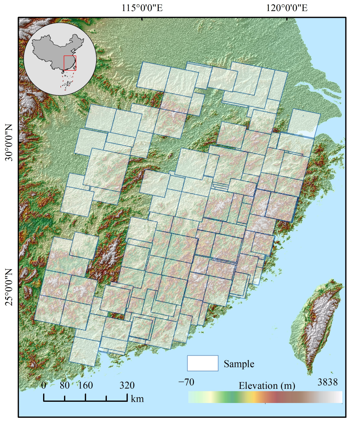
Figure 1. Study area and locations of the 292 SCC samples from the Landsat-8 scenes.
Remotesensing 15 05542 g001
Figure 2. (a) A real-color composite sample. (b) The result after applying the NDVI and the whiteness tests. (c,d) The results before and after applying the morphological opening. The region of (c,d) is shown with the red rectangle in (e). Such a small area is shown in (c,d) for clarity. (e) The final result of the cloud identification. This sample is for 29 July 2014.
Remotesensing 15 05542 g002
Figure 3. The original CSD (dotted), and the fitted CSD (yellow line) obtained using piecewise regression for a sample on 29 July 2014. The dashed line shows a reference line with an exponent of −1.7.
Remotesensing 15 05542 g003
Figure 4. Histogram of scale breaks for the 292 SCC samples.
Remotesensing 15 05542 g004
Figure 5. CSDs of all samples. (a) The original CSDs. (b) The CSDs where cloud sizes are normalized by scale breaks and cloud numbers are normalized by N 0 ~ . (c) The CSDs where clouds sizes are normalized by scale breaks and cloud numbers are normalized by N 0.2 ~ 1 .
Remotesensing 15 05542 g005
Figure 6. The box-whisker plots of coefficients b 1 and b 2 in Equation (8).
Remotesensing 15 05542 g006
Figure 7. (a) The variation of the normalized cloud number density with the normalized elevation. (b) The variation of the cloud number density relative to the cloud number density of the first bin of the normalized elevation.
Remotesensing 15 05542 g007
Figure 8. The variation of the normalized cloud size with the normalized elevation.
Remotesensing 15 05542 g008
Table 1. Landsat-8 bands used in this study. NIR is near infrared, SWIR is shortwave infrared, and TIR is thermal infrared.
Band NumberBand NameWavelength (μm)Resolution (m)Sensor
2Blue0.452 ~ 0.51230OLI
3Green0.533 ~ 0.59030OLI
4Red0.636 ~ 0.67330OLI
5NIR0.851 ~ 0.87930OLI
6SWIR11.566 ~ 1.65130OLI
7SWIR22.107 ~ 2.29430OLI
10TIR10.60 ~ 11.19100TIRS
Disclaimer/Publisher’s Note: The statements, opinions and data contained in all publications are solely those of the individual author(s) and contributor(s) and not of MDPI and/or the editor(s). MDPI and/or the editor(s) disclaim responsibility for any injury to people or property resulting from any ideas, methods, instructions or products referred to in the content.