Technical Note

Using Downwelling Far- and Thermal-Infrared Hyperspectral Radiance for Cloud Phase Classification in the Antarctic

1
College of Meteorology and Oceanography, National University of Defense Technology, Changsha 410073, China
2
High Impact Weather Key Laboratory of CMA, Changsha 410073, China
*
Author to whom correspondence should be addressed.
Remote Sens. 2024, 16(1), 71; https://doi.org/10.3390/rs16010071
Submission received: 30 October 2023 / Revised: 12 December 2023 / Accepted: 18 December 2023 / Published: 23 December 2023
(This article belongs to the Special Issue Remote Sensing of Aerosols, Planetary Boundary Layer, and Clouds)

Abstract

:
The cloud phase is one of the most important parameters of clouds. In this paper, we propose a method for cloud phase classification that synergistically utilizes the far- and thermal-infrared bands based on the Atmospheric Emitted Radiance Interferometer (AERI) at the Atmospheric Radiation Measurement West Antarctic Radiation Experiment (AWARE) observatory in 2016. The possible features in the far- and thermal-infrared bands are analyzed based on the differences in the simulated cloud brightness temperature (BT) spectra with different cloud phases. Using the support vector machine (SVM) algorithm, four features are determined to identify the cloud phase, which include the BT at 900 cm−1, the slope of the fitted function of BT in the 900–1000 cm−1 interval, the BT difference (BTD) between 512 cm−1 and 726 cm−1, and the BTD between 550 cm−1 and 726 cm−1. Here, the performance of the proposed method is evaluated with Shupe’s and Turner’s method. The monthly average accuracy of the proposed method, the method without the two far-infrared features, and Turner’s method are about 76%, 36%, and 49%, respectively, which infer the good performance of the proposed method and also indicate that the far-infrared band features can effectively enhance cloud phase classification. It is notable that, compared to Shupe’s method, the accuracy for the proposed method is only 61% during the Antarctic summer, which results from the definitions of cloud phase and radiative effect. In addition, the accuracy is only 44% for Turner’s method in seasons with a low frequency of mixed clouds due to the significant effect of water vapor.

Graphical Abstract

1. Introduction

Clouds have a significant effect on the Earth’s radiative budget and climate change [1]. The feedback processes associated with clouds and the impact of clouds on heating or cooling the atmosphere are quite complex [2]. For example, cloud phase, particle size distribution, and concentration affect the transmission of longwave radiation (i.e., cloud radiation effects), dramatically impacting the Earth’s climate system [3]. Cloud phase, among them, is a prerequisite for studying cloud microphysical properties and largely determines a cloud’s radiation effects [4]. The incorrect classification of cloud phases may lead to large retrieval errors (20–100%) in optical depth and effective particle radius, which convert into errors of 5–20% in downwelling longwave fluxes [5]. There are still large uncertainties in assessing the impact of clouds on the Earth’s radiation budget (ERB) [1,6]. There are observable fast-warming phenomena in the Antarctic troposphere, and clouds play a great impact on this aspect of climate change [7]. However, little is known about the clouds in the Antarctic, an isolated and harsh place, due to the challenges in deploying instruments and the constraints of traditional satellite passive remote sensing techniques [8,9,10]. Therefore, accurately identifying cloud phases is significant for understanding cloud radiation effects and evaluating the ERB in the Antarctic.
There have been many studies on cloud phase classification. ISCCP [11] used clouds top pressure and temperature to classify them into ice and liquid water clouds, but, in fact, cloud phase is not entirely determined by these two parameters. A more widespread cloud phase classification method mainly uses the depolarization ratio based on active remote sensing instruments, where the depolarization ratio of liquid water is close to 0, and the depolarization ratio of ice is larger [12,13]. However, the empirical threshold based on a single instrument in this method may cause significant errors. Based on this, Shupe [14] proposed to combine the ground-based millimeter-wave cloud radar, polarized lidar, microwave radiometer, and radiosonde to classify polar cloud phases and set thresholds based on physical principles and observation data to classify atmospheric features into ice clouds, mixed-phase clouds, liquid water clouds, precipitation, and aerosols, which is a more accurate classification method not limited by region or time. Nevertheless, this method relies on multiple ground-based observation instruments, and setting thresholds requires long-term observation data. In addition, some studies have suggested that cloud phase classification can be based on passive remote sensing measurement data, for example, by using the difference in absorption between ice and water in the infrared band: the absorption coefficients of ice and water are almost equal in the 1000–1250 cm−1 (8–10 µm) range, while the absorption coefficient of ice is larger than that of water in the 750–1250 cm−1 (10–13 µm) range. This phenomenon leads to the difference in brightness temperature (BT) of different cloud phases. According to this physical foundation, Ackerman et al. [15] first proposed a tri-spectral cloud phase classification method based on 833 cm−1 (12 µm), 910 cm−1 (11 µm), and 1250 cm−1 (8 µm) spectra. On this basis, Strabala et al. [16] further established an algorithm for cloud phase classification at the 833 cm−1 (12 µm), 910 cm−1 (11 µm), and 1176 cm−1 (8.5 µm) spectra. Both of them used BT difference (BTD) for the analysis. Dan Lubin [17] used BT slope (BTS) for cloud phase classification based on 800–1204 cm−1 (8.3–12.5 µm) hyperspectral infrared radiation data, which performed well. However, this method is sensitive to water vapor absorption, and inaccurate measurement of the humidity profile can easily cause errors in cloud phase identification. Focusing on a narrow window with particularly small water vapor absorption, Garrett et al. [18] proposed a cloud phase retrieval algorithm based on 862.5 cm−1, 935.8 cm−1, and 988.4 cm−1 spectra that classified clouds into ice, liquid water, and indeterminate cases by exploiting the difference in the emissivity of ice and water particles within the atmospheric window region. This algorithm is able to retrieve optically thin non-blackbody clouds, but its performance is affected by the temperature at cloud base height and stratospheric ozone profile measurement errors. Methods of classifying cloud phases based on infrared spectra are relatively reliable, but most of them are limited to the thermal-infrared band of 750–1250 cm−1 (8–13 µm) spectra and do not fully utilize the far-infrared region.
The far-infrared (FIR) spectral band is essential to the radiation spectrum, ranging from about 100 to 667 cm−1 (15–100 µm) spectra [19]. The equivalent blackbody temperature of the Earth is 255 K, whose peak energy occurs at about 500 cm−1 in the FIR [20]. But, until the end of the last century, due to the limitations of observation technology on various platforms, research on this band was still relatively lacking [21,22]. In recent years, significant progress has been made in the high-resolution observation of radiation in the FIR, including multiple platforms such as satellite, airborne, and ground-based [23]. Many studies have shown that the FIR is highly sensitive to clouds and water vapor [24]. In this band, water absorption is greater than ice, and the atmosphere is transparent enough to supply the measurement and retrieval in the thermal-infrared band, thereby improving the accuracy of cloud detection and water vapor profile retrieval [25,26]. For example, Turner et al. [27] chose the slope of the emissivity of 800–900 cm−1 (11–12.5 µm) spectra, the ratio of the average cloud emissivity from 526–588 cm−1 (17–19 µm) to 833–909 cm−1 (11–12 µm) spectra, and the difference between the average cloud emissivity from 526–588 cm−1 to 833–909 cm−1 spectra to classify cloud phases as ice, mixed, liquid water, and opaque clouds, but this classification method is not applicable to cases with high water vapor and large optical depth (above about 5). In addition, some studies determined cloud phases based on machine learning algorithms. For example, Maestri et al. [23] used a supervised features’ selection algorithm to find out the most sensitive BTDs for the determination of the full spectral band. This approach is simple and efficient, but it relies excessively on statistical patterns among the data and ignores the physical information of the ice and liquid water cloud spectra. Thus, this study establishes a cloud phase classification method based on the ice and liquid water clouds BT spectra with the AERI, utilizing the far-infrared band to reduce the effect of water vapor.
The organization of this paper is as follows. Section 2 introduces the instruments and data used in this paper. Section 3 proposes a new method for cloud phase determination. Section 4 presents the results of the proposed method and analyzes the results by individual case. Section 5 provides a summary.

2. Instruments and Data
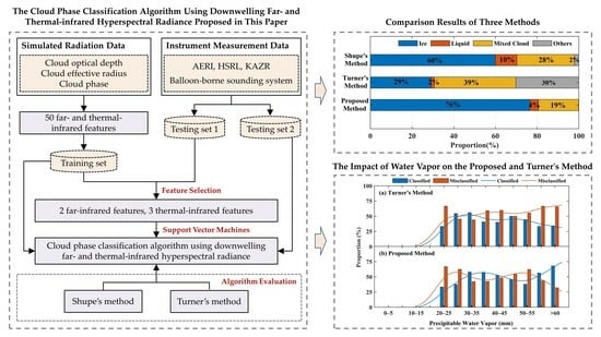
The Atmospheric Radiation Measurement (ARM) conducted a climate-related field campaign in West Antarctica, the ARM West Antarctic Radiation Experiment (AWARE), to study the surface energy balance and global climate patterns in the Antarctic [28]. This study uses observational data from McMurdo Station (77°51′S, 166°40′E) in the AWARE from January to December 2016, including the data obtained with AERI, the High Spectral Resolution Lidar (HSRL), the Ka-band ARM zenith radar (KAZR), and sounding reanalysis data [29].
The Atmospheric Emitted Radiance Interferometer (AERI) deployed at McMurdo Station is a passive, fully automated, ground-based Fourier-Transform Spectrometer (FTS) developed by the University of Wisconsin Space Science and Engineering Center (UW-SSEC) for the ARM program, which is used to measure the downwelling radiance of the sky directly above the instrument [30,31]. The spectrum measurement range of the AERI is between 400 and 3300 cm−1 (3–25 μm) with a spectral resolution of 0.5 cm−1, and the field of view of the instrument is 1.3°. The AERI collects data every 20 s in rapid sampling mode, providing the vertical profiles of clouds and aerosols’ temperature, humidity, and infrared spectral properties [32,33].
The High Spectral Resolution Lidar (HSRL) system is designed for long-term unattended operation, controlled remotely, and operation as an Internet-enabled device [34]. With a small field of view and a narrow optical bandwidth, the HSRL uses the spectral distribution of the laser backscatter signal to distinguish aerosol and molecular signals, thus improving atmospheric parameters retrieval accuracy [35]. The HSRL deployed at McMurdo Station has a temporal resolution of 30 s and a vertical resolution of 30 m and can provide vertical profiles of optical depth, depolarization ratio, and backscatter coefficient [36,37].
The Ka-band ARM zenith radar (KAZR) deployed at McMurdo Station is a zenith-pointing Doppler cloud radar operating at approximately 35 GHz. The main purpose of the KAZR is to provide vertical profiles of clouds by measuring the first three Doppler moments (reflectivity, radial Doppler velocity, and spectra width) at a range resolution of approximately 30 m from near-ground to nearly 20 km in altitude [38].
The balloon-borne sounding system (SONDE) includes fixed ground stations and disposable radiosondes, which provide vertical profiles of temperature, pressure, relative humidity, wind direction, and wind speed [28,39]. AWARE launches balloons four times a day. This study uses interpolated sounding data with a time resolution of 1 min and an altitude range of ground to 25–30 km. The temperature and pressure resolutions are 0.1 K and 0.1 hPa, respectively [40,41].

3. Method

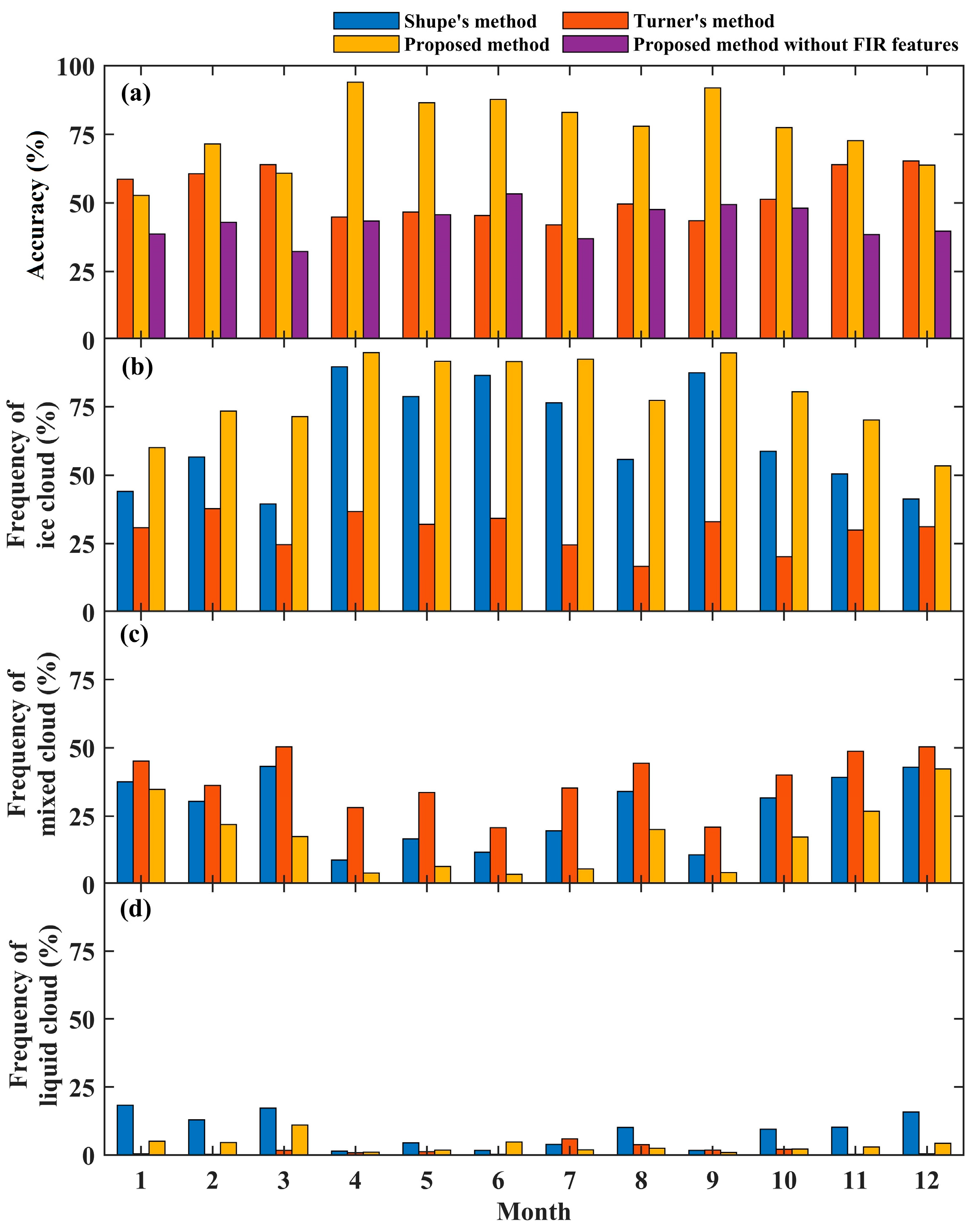
3.1. The Features Selection

In this study, the line-by-line radiative transfer model (LBLRTM) combined with discrete ordinate radiative transfer (DISORT) is used to simulate the infrared hyperspectral radiative properties of clouds [42]. Using the atmospheric profile at 01:48 UTC on the 5 January 2016, ice and liquid water clouds radiation with different cloud optical depths and effective particle radius is simulated and converted into BT using the following equation:
T B = b × υ log 1 + a × υ 3 I
where I is the radiance in mW/(m2 sr cm−1); ν is the wavenumber; a and b are constants of 1.191 × 10⁻⁵ and 1.439, respectively; and TB is the brightness temperature in K. The hyperspectral BT data for optical depths of 0.2, 1.0, and 8.0 and three sets of effective particle radius for liquid water (reff,w) and ice (reff,i) clouds (reff,w = 5 µm and reff,i = 20 µm, reff,w = 7 µm and reff,i = 30 µm, reff,w = 10 µm and reff,i = 50 µm) are shown in Figure 1.
From Figure 1, the BT of ice and liquid water clouds differ significantly at different intervals. For example, in the region of 400–600 cm−1, the BT of liquid water clouds is higher than that of ice clouds, and, in the region of 800–1200 cm−1, the BT variation of liquid water clouds is more moderate than that of ice clouds. By combining this with the simulated BT data, “features” that are sensitive to cloud phase are selected to distinguish between ice and liquid water clouds, where “features” refers to the difference, ratio, or slope of the BT in different narrow spectral regions. Preliminarily, 50 features are selected empirically according to the simulated BT data and are listed in Appendix A.
To reduce the effect of water vapor, simulated BT data of ice and liquid water clouds at different specific humidity are considered. Taking the ice phase as an example, Figure 2 shows the simulated ice cloud BT spectra for both high and low specific humidity cases. Based on this, the features that are highly influenced by water vapor are removed from the 50 possible features selected.
To further evaluate the ability of the selected feature pairs to determine cloud phases, the classification accuracy of different numbers of features is studied, where “accuracy” refers to the comparison between the results of the proposed and Shupe’s methods. The result shows that the accuracy is low when the number of features is below three (the monthly average classification accuracy is below 60%, with only 35% in January), and the cloud phase classification accuracy decreases due to excessive redundancy when the number of features is above four (the monthly average classification accuracy is below 70%, with only 43% in January). Considering the efficiency and classification accuracy, the number of feature combinations is four. Finally, features 1, 6, 41, and 44 are determined as the final features for identifying cloud phases in this study, which are the BT at 900 cm−1, the slope of the BT fitted function in the 900–1000 cm−1 interval, the BTD between 512 cm−1 and 726 cm−1, and the BTD between 550 cm−1 and 726 cm−1, where features 41 and 44 are FIR features. Considering that the simulated cloud brightness temperature (CBT) is hardly below 170 K, clouds with CBT less than 170 K at 900 cm−1 are considered indistinguishable cases and removed in the measurement data.

3.2. The Classification Method

For the training set, the 270 group samples are built with the optical depth and effective radius of the different cloud phases. The parameters are set as follows: the optical depths are 0.2, 0.4, 0.6, 0.8, 1.0, 1.5, 2.0, 2.5, 3.0, 3.5, 4.0, 5.0, 6.0, 7.0, and 8.0; the effective radii of the ice cloud particles are 10, 20, 30, 50, 70, and 100 µm; the effective radii of the liquid water cloud particles are 2, 3, 5, 7, 10, and 15 µm; and the effective radii of the mixed cloud particles are (reff,w = 3 µm, reff,i = 20 µm), (reff,w = 3 µm, reff,i = 30 µm), (reff,w = 5 µm, reff,i = 30 µm), (reff,w = 7 µm, reff,i = 20 µm), (reff,w = 7 µm, reff,i = 30 µm), and (reff,w = 10 µm, reff,i = 40 µm). To simulate the observed conditions, the mixed clouds are composed of different optical depth ratios of ice and water particles (from 1:9 to 9:1), respectively, and homogeneous mixing. In this article, clouds are classified as mixed clouds when the optical depth of both ice and water is greater than 10%. If the optical depth of ice (water) is greater than 10% and that of water (ice) is less than 10%, the cloud is classified as an ice (liquid water) cloud, which is the same as in Turner’s method [27]. The test set is constructed using AWARE measurement data in 2016, with the results of Shupe’s method as the true values.
The support vector machines (SVM) have good generalization and high computational efficiency [43,44]. In this study, the SVM algorithm is used to construct the mapping relationship between BT spectral features and cloud phases in the training and testing processes.

4. Results and Discussion
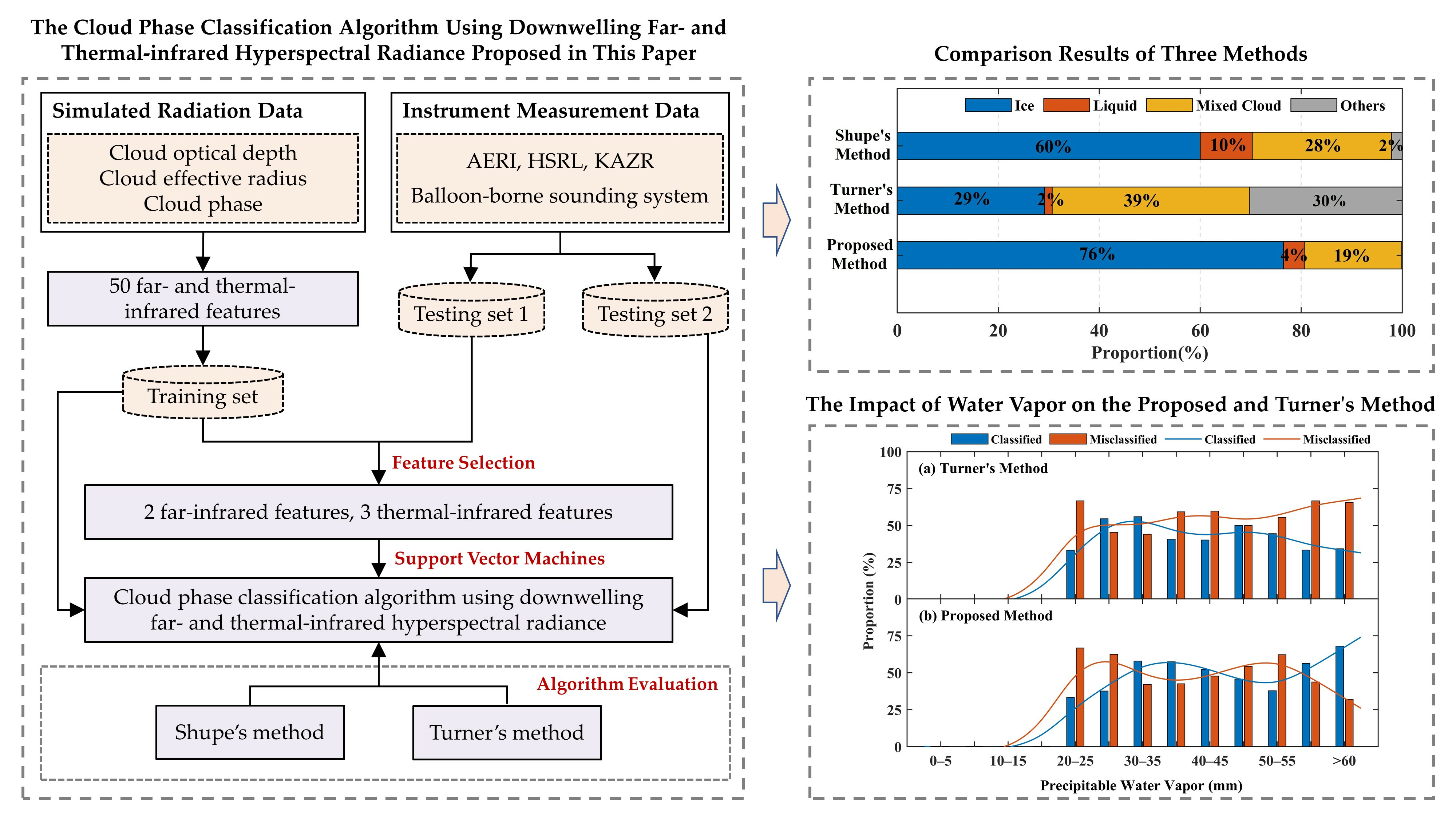
4.1. Results

The data with clouds during the AERI observation period are selected based on the lidar cloud base height, and then the phase classification is evaluated using Shupe’s and Turner’s methods, respectively. Since Shupe’s method obtains the vertical profile of cloud phases, it needs to be further processed for evaluation. If there is more than one cloud phase in the cloud profile and the cloud pixel points of each phase account for more than 30% of the total cloud pixels, it is considered a mixed cloud. In the profiles with the other cloud phase conditions, it is the cloud phase with the highest proportion. If there is rain, snow, or drizzle, this profile is judged as precipitation and removed from the evaluation sample. If there is no cloud or no precipitation, it is a clear sky and can be ignored in the evaluation [45].
Shupe’s method is a popular cloud phase classification method and can be thought as the true value for evaluating the proposed method in this study. The occurrence frequencies of ice, mixed, and liquid water clouds in each month for the three methods as well as the accuracy of Turner’s and the proposed methods compared with Shupe’s method are shown in Figure 3. From Figure 3a, the accuracy of Turner’s method is around 50% in each month. Among them, the accuracy grows to 55% in the Antarctic summer and autumn (from November to March), which are the months with a higher frequency of mixed cloud occurrence. Compared with Turner’s method, the proposed method agrees better with Shupe’s, where the accuracy rate is more than 75%, except for the Antarctic summer (from December to February), and more than 85% in autumn and winter.
To further verify the role of the far-infrared band in cloud phase identification, the accuracy of the method without the two far-infrared features among the four selected features (only feature 1 and 2) is considered. As shown in Figure 3a, the accuracy of the proposed method with four features is 77%, which is higher than the accuracy of the method without the two far-infrared features, i.e., 43%. This infers the good performance of the proposed method and also indicates that the far-infrared band features can effectively enhance cloud phase classification. From Figure 3b–d, the McMurdo Station is dominated by ice clouds, with a proportion of more than 40% and up to 75% in autumn and winter (from April to September). In contrast, the mixed and liquid water clouds occur more frequently in spring and summer (from October to March), accounting for about 30% and 15%, respectively, while their percentage decreases significantly in other seasons. The above results indicate that the ice phase is the main cloud phase in the Antarctic, and the frequency of different phases of clouds varies greatly with the seasons. It is noticeable that the average agreement rate is only 63% for the proposed method in the Antarctic summer (from December to February) and 45% for Turner’s method in seasons with a low frequency of mixed clouds (autumn and winter, from April to September). In December, Shupe’s method classified 41% of all cloud profiles as ice clouds, 43% as mixed clouds, and 16% as liquid water clouds. From Figure 3b–d, the proposed method identifies 53% of the samples as ice clouds and 42% and 4% as mixed and liquid water clouds, respectively. Meanwhile, Turner’s method identifies 50% of the cloud profile samples as mixed clouds, similar to Shupe’s results, but can only identify 31% of ice cloud samples and can hardly detect liquid water clouds.
To deeply analyze the identification error of Turner’s and the proposed method for the cloud phases in the Antarctic summer, the data in December are selected for the study. The total cloud phase samples are 10,906. The detailed results of the classification are shown in Table 1, where “other samples” represent situations which cannot be recognized. From Figure 3 and Table 1, it can be concluded that the main reason for the low accuracy of Turner’s and the proposed method in December is the failure to identify the ice and liquid water clouds effectively. To investigate the reasons further, the sample data of ice and liquid water clouds misclassified by the two methods are compared with the classification thresholds or features, respectively. As in Figure 4, according to Turner’s method, a sample is considered as the ice (liquid water) cloud if it lies within the ice (liquid water) cloud feature region and the mixed cloud if it lies between the ice and liquid water cloud thresholds. Finally, the classification results of the three thresholds are considered together to determine the sample phase. From Figure 4, it can be found that the misclassification of the liquid water cloud in Turner’s method is mainly due to the fact that the average cloud emissivity in the 526–588 cm−1 region is lower than that in the 833–909 cm−1 region, leading to a misclassified results. The misclassified ice cloud samples are similar, but the values in the 526–588 cm−1 region are larger than those in the 833–909 cm−1 region. The proportion of cloud samples correctly classified and misclassified by Turner’s and the proposed methods within different precipitable water vapor (PWV) intervals are given in Figure 5, where the blue color indicates the proportion of correctly classified cloud samples by Turner’s method, and the red indicates the misclassification. It can be seen that, as PWV increases, the proportion of samples correctly identified by Turner’s method in each interval decreases, and more samples are misidentified, which indicates that Turner’s method is highly affected by water vapor. The distribution of the ice and liquid water cloud data misclassified by the proposed method is shown in Figure 6, and the proportion of cloud samples in PWV intervals is shown in Figure 5. According to Figure 5, the proportion correctly identified by the proposed method fluctuates with the increase in PWV, but the overall change is smoother than that obtained with Turner’s method. Therefore, it can be assumed that the proposed method is not significantly affected by water vapor.
Based on this, the following studies are carried out in order to investigate the impact of water vapor on Turner’s and the proposed methods. The PWV of the measured data is divided into seven intervals, ranging from small to large, and the accuracy of Turner’s and the proposed methods in identifying cloud phases in different intervals is studied. According to the measured data of AWARE, PWV is divided into seven intervals, i.e., 0–10, 10–15, 15–20, 20–25, 25–30, 30–35, and above 35 mm. As shown in Figure 7, the accuracy of Turner’s method is about 80% when the PWV is under 10 mm and decreases to 45% as the PWV increases to 15 mm. When PWV continued to increase, there is a small increase in accuracy, up to about 60%, and then it rapidly decreases to around 40%. For the proposed method, the accuracy is almost maintained at about 75%, with small fluctuations. The above results indicate that Turner’s method is sensitive to water vapor, while the proposed method is not significantly affected by water vapor. A more detailed analysis will be discussed in Section 4.2.

4.2. Case Analysis

To further analyze the results of the proposed methods in Section 4.1, the case at McMurdo Station on December 25th is selected to compare and analyze the cloud phase results identified by the three methods.
The HSRL, KAZR, and the radiosonde measurements from 08:00 to 24:00 UTC on December 25th are given in Figure 8, with the classification results obtained by Shupe’s, Turner’s, and the proposed methods. It can be seen that, at 08:00–14:00 UTC, there is a layer of ice cloud with a low backscatter coefficient and a high depolarization ratio at an altitude of about 1–3 km, with a reflectivity of −12 dBZ. At the same time, there are discontinuous clouds with a thickness of about 0.1 km above it, with a reflectivity of about −20 dBZ. Based on the HSRL measurement, they can be determined as ice clouds. During this period, the cloud phase classification results of Shupe’s method are mainly ice clouds, with a small number of mixed clouds. The results of Turner’s method are basically consistent with Shupe’s, except for some unrecognized samples. In contrast, the proposed method classifies all the clouds as mixed clouds, accompanied by a few ice clouds. At 17:00–18:00 UTC, a layer of liquid water clouds appears at about 3 km and gradually dissipates. There are discontinuous multi-layer clouds at 2–3 km, with low backscatter coefficient and depolarization ratio and a reflectivity of about −30 dBZ. During this time frame, Shupe’s method identifies all the clouds as liquid water clouds, which is inconsistent with the detection results of the HSRL and KAZR systems. Turner’s method identifies the clouds as ice clouds, and the results of the proposed method are mixed clouds. At 18:00–21:00 UTC, the HSRL and KAZR measurements show mixed clouds with a thin liquid water cloud in the upper layer and a thick ice cloud in the lower layer. At 22:00–24:00 UTC, the clouds are similar to those at 18:00–21:00 UTC, with a lower ice cloud base height of 1 km and a thickness of 1 km. The height of the upper water cloud gradually extends to 3 km, and the cloud layer is discontinuous. During this time, Shupe’s method identifies the results mainly as liquid water clouds, Turner’s method as ice and mixed clouds, and the proposed method mostly as mixed clouds.
Comparing Figure 8e–g, the results of the three methods are not completely consistent. Although the results of Shupe’s method are taken as the true values in this paper, the combination of the HSRL and KAZR detection results reveals that this method can also lead to misclassification (e.g., 17:00–18:00, 23:00–24:00 UTC in Figure 8. The presence of both ice and liquid water in the clouds during this time period should be classified as mixed clouds; however, the results of Shupe’s method are water clouds). In addition, Turner’s and the proposed methods classify cloud phases based on the ratio of the optical depths of ice and water. A cloud will be classified as a mixed cloud when the optical depths of ice and water are greater than 10%, which is different from the definition of cloud phases in Shupe’s method. The different definitions of cloud phases by the three methods also lead to variations in the classification results (e.g., 08:00–12:00 UTC). For Turner’s method, the specific humidity is high during the Antarctic summer (about 1.2 g/kg at cloud height, as shown in Figure 8h), and the accuracy of this method is significantly decreased, owing to the influence of water vapor, resulting in a poor performance. The proposed method, on the other hand, performs well as PWV increases and, therefore, is more consistent with Shupe’s method, with better results. Moreover, since the proposed method uses BT to identify cloud phases, the cloud phase classification results are radiometric, not physical [18]. The above-mentioned analysis results of the case are also consistent with Section 4.1.

5. Conclusions

In this study, we establish a cloud phase classification method synergistically using the far- and thermal-infrared bands based on AERI, with four cloud brightness temperature spectral features according to the sensitivity of the far- and thermal -infrared regions to cloud phases, and compare the results with Shupe’s and Turner’s methods to evaluate the reliability of the proposed method in this study.
In this paper, the brightness temperature at 900 cm−1, the slope of the fitted function of brightness temperature in the 900–1000 cm−1 interval, the brightness temperature difference between 512 cm−1 and 726 cm−1, and the brightness temperature difference between 550 cm−1 and 726 cm−1 are selected as the features that can identify cloud phases more accurately with the far-infrared band features. The accuracy of the proposed method with four features is 77%, which is higher than the accuracy of the method without the two far-infrared features, i.e., 43%, and that of Turner’s method, i.e., 53%. This infers the good performance of the proposed method and the ability of the far-infrared band to detect cloud phases. The results indicate that the cloud phase is mainly composed of ice and that the frequency of different cloud phases varies significantly with seasons in the Antarctic. During the observation period, the proposed method agrees with the Shupe’s method by more than 75%, which is higher than Turner’s method. In addition, Turner’s method is sensitive to water vapor, and the proposed method is not significantly affected by water vapor. The accuracy of Turner’s method is about 80% when the PWV is under 10 mm and decreases rapidly to 40% as the PWV increases. In comparison, the proposed method consistently performs well, with an accuracy of about 75%. The data on misclassifications by both methods are further analyzed: the misclassification of Turner’s method is caused by the influence of water vapor and cloud phase definitions, while the proposed method misclassified data not only due to the influence of definitions, but also because its results are in the meaning of “radiation”.
The work in this study is carried out based on Antarctic data, which have some regional limitations. Future studies can be conducted in the Arctic and mid-latitudes to validate and extend the cloud phase classification method proposed in this paper. In addition, the impact of factors such as aerosols on the proposed method will be further investigated in future works.

Author Contributions

Methodology, L.L.; software, H.R. and J.Y.; validation, H.X.; writing—original draft preparation, H.R.; writing—review and editing, H.X. and J.Y.; supervision, L.L. All authors have read and agreed to the published version of the manuscript.

Funding

This research was funded by the National Key Research and Development Program of China (Grant 2021YFC2802501), the National Natural Science Foundation of China (Grant 41875025), and the Hunan Provincial Natural Science Foundation of China (Grant 2021JJ10047).

Data Availability Statement

The data of the AWARE (including AERI, HSRL, etc.) can be downloaded at https://adc.arm.gov/discovery/#/.

Conflicts of Interest

The authors declare no conflict of interest.

Appendix A

Table A1. The 50 features selected in this article are as follows, where BTR indicates the brightness–temperature ratio, BTD the difference, and STD the standard deviation.
1BT at 900 cm−118BTR of 935.8 to 988.4 cm−135BTD of 420 to 550 cm−1
2BTR of 496 to 513 cm−119BTR of 420 to 512 cm−136BTD of 420 to 589 cm−1
3BTR of 496 to 532 cm−120BTR of 420 to 550 cm−137BTD of 420 to 726 cm−1
4BTR of 558 to 482 cm−121BTR of 420 to 589 cm−138BTD of 420 to 778 cm−1
5Ratio of the BT sum of 532, 553, 573.5 cm−1 to the BT sum of 596, 608.5 cm−122BTRR of 420 to 726 cm−139BTD of 512 to 550 cm−1
6Slope of the fitted function of BT in the 800–900 cm−1 interval23BTR of 420 to 778 cm−140BTD of 512 to 589 cm−1
7Slope of the fitted function of BT in the 900–1000 cm−1 interval24BTR of 512 to 550 cm−141BTD of 512 to 726 cm−1
8BTR of 558 to 495 cm−125BTR of 512 to 589 cm−142BTD of 512 to 778 cm−1
9BTR of 532 to 553 cm−126BTR of 512 to 726 cm−143BTD of 550 to 589 cm−1
10Ratio of the BT sum of 532, 553, 573.5 cm−1 to the BT sum of 428, 496.5 cm−127BTR of 512 to 778 cm−144BTD of 550 to 726 cm−1
11Ratio of the BT sum of 428, 496.5 cm−1 to the BT sum of 596, 608.5 cm−128BTR of 550 to 589 cm−145BTD of 550 to 778 cm−1
12Ratio of the BT sum of 428, 496.5, 532, 553, 573.5 cm−1 to the BT sum of 596, 608.5 cm−129BTR of 550 to 726 cm−146BTD of 589 to 726 cm−1
13Ratio of the BT sum of 478, 489 cm−1 to the BT sum of 774, 778 cm−130BTR of 550 to 778 cm−147BTD of 589 to 778 cm−1
14Ratio of the BT product of 478, 489 cm−1 to the BT product of 774, 778 cm−131BTR of 589 to 726 cm−148BTD of 726 to 778 cm−1
15Ratio of the BT sum of 400, 460.5 cm−1 to the BT sum of 874, 940 cm−132BTR of 589 to 778 cm−149STD of BT in the 528–552 cm−1 interval
16Ratio of the BT product of 400, 460.5 cm−1 to the BT product of 874, 940 cm−133BTR of 726 to 778 cm−150STD of BT in the 500–550 cm−1 interval
17BTR of 862.5 to 935.8 cm−134BTD of 420 to 512 cm−1

References

  1. Peterson, C.A.; Huang, X.; Chen, X.; Yang, P. Synergistic Use of Far- and Mid-Infrared Spectral Radiances for Satellite-Based Detection of Polar Ice Clouds Over Ocean. J. Geophys. Res. Atmos. 2021, 127, 1–20. [Google Scholar] [CrossRef]
  2. Martinazzo, M.; Magurno, D.; Cossich, W.; Serio, C.; Masiello, G.; Maestri, T. Assessment of the accuracy of scaling methods for radiance simulations at far and mid infrared wavelengths. J. Quant. Spectrosc. Radiat. Transf. 2021, 271, 107739. [Google Scholar] [CrossRef]
  3. Lachlan-Cope, T. Antarctic clouds. Polar Res. 2010, 29, 150–158. [Google Scholar] [CrossRef]
  4. Matus, A.V.; L’Ecuyer, T.S. The role of cloud phase in Earth’s radiation budget. J. Geophys. Res. Atmos. 2017, 122, 2559–2578. [Google Scholar] [CrossRef]
  5. Key, J.R.; Intrieri, J.M. Cloud particle phase determination with the AVHRR. J. Appl. Meteorol. 2000, 39, 1797–1804. [Google Scholar] [CrossRef]
  6. Di Natale, G.; Turner, D.D.; Bianchini, G.; Del Guasta, M.; Palchetti, L.; Bracci, A.; Baldini, L.; Maestri, T.; Cossich, W.; Martinazzo, M.; et al. Consistency test of precipitating ice cloud retrieval properties obtained from the observations of different instruments operating at Dome-C (Antarctica). Atmos. Meas. Tech. 2022, 15, 7235–7258. [Google Scholar] [CrossRef]
  7. Silber, I.; Verlinde, J.; Eloranta, E.W.; Cadeddu, M. Antarctic Cloud Macrophysical, Thermodynamic Phase, and Atmospheric Inversion Coupling Properties at McMurdo Station: I. Principal Data Processing and Climatology. J. Geophys. Res. Atmos. 2018, 123, 6099–6121. [Google Scholar] [CrossRef]
  8. Bromwich, D.H.; Nicolas, J.P.; Hines, K.M.; Kay, J.E.; Key, E.L.; Lazzara, M.A.; Lubin, D.; McFarquhar, G.M.; Gorodetskaya, I.V.; Grosvenor, D.P.; et al. Tropospheric clouds in Antarctica. Rev. Geophys. 2012, 50, RG1004. [Google Scholar] [CrossRef]
  9. Lawson, R.P.; Gettelman, A. Impact of Antarctic mixed-phase clouds on climate. Proc. Natl. Acad. Sci. USA 2014, 111, 18156–18161. [Google Scholar] [CrossRef] [PubMed]
  10. Di Natale, G.; Bianchini, G.; Del Guasta, M.; Ridolfi, M.; Maestri, T.; Cossich, W.; Magurno, D.; Palchetti, L. Characterization of the Far Infrared Properties and Radiative Forcing of Antarctic Ice and Water Clouds Exploiting the Spectrometer-LiDAR Synergy. Remote Sens. 2020, 12, 3574. [Google Scholar] [CrossRef]
  11. Roscow, W.B.; Schiffer, R.A. Advances in Understanding Clouds from ISCCP. Bull. Am. Meteorol. Soc. 1999, 80, 2261–2288. [Google Scholar] [CrossRef]
  12. Sassen, K. The Polarization Lidar Technique for Cloud Research: A Review and Current Assessment. Bull. Am. Meteorol. Soc. 1991, 72, 1848–1866. [Google Scholar] [CrossRef]
  13. Hu, Y.-X.; Winker, D.; Yang, P.; Baum, B.; Poole, L.; Vann, L. Identification of cloud phase from PICASSO-CENA lidar depolarization: A multiple scattering sensitivity study. J. Quant. Spectrosc. Radiat. Transf. 2001, 70, 569–579. [Google Scholar] [CrossRef]
  14. Shupe, M.D. A ground-based multisensor cloud phase classifier. Geophys. Res. Lett. 2007, 34, L22809. [Google Scholar] [CrossRef]
  15. Ackerman, S.A.; Smith, W.L.; Spinhirne, J.D.; Revercomb, H.E. The 27–28 October 1986 FIRE IFO cirrus case study:Spectral properties of cirrus clouds in the 8-12 μm window. Mon. Weather Rev. 1990, 118, 2377–2388. [Google Scholar] [CrossRef]
  16. Strabala, K.I.; Ackerman, S.A. Cloud Properties inferred from 8-12 µm Data. J. Appl. Meteorol. 1994, 33, 212–229. [Google Scholar] [CrossRef]
  17. Lubin, D. Thermodynamic phase of maritime Antarctic clouds from FTIR and supplementary radiometric data. J. Geophys. Res. Atmos. 2004, 109, D04204. [Google Scholar] [CrossRef]
  18. Garrett, T.J.; Zhao, C. Ground-based remote sensing of thin clouds in the Arctic. Atmos. Meas. Tech. 2013, 6, 1227–1243. [Google Scholar] [CrossRef]
  19. Magurno, D.; Cossich, W.; Maestri, T.; Bantges, R.; Brindley, H.; Fox, S.; Harlow, C.; Murray, J.; Pickering, J.; Warwick, L.; et al. Cirrus Cloud Identification from Airborne Far-Infrared and Mid-Infrared Spectra. Remote Sens. 2020, 12, 2097. [Google Scholar] [CrossRef]
  20. Harries, J.; Carli, B.; Rizzi, R.; Serio, C.; Mlynczak, M.; Palchetti, L.; Maestri, T.; Brindley, H.; Masiello, G. The Far-infrared Earth. Rev. Geophys. 2008, 46, RG4004. [Google Scholar] [CrossRef]
  21. Di Natale, G.; Palchetti, L. Sensitivity studies toward the retrieval of ice crystal habit distributions inside cirrus clouds from upwelling far infrared spectral radiance observations. J. Quant. Spectrosc. Radiat. Transf. 2022, 282, 108120. [Google Scholar] [CrossRef]
  22. Maestri, T.; Rizzi, R.; Tosi, E.; Veglio, P.; Palchetti, L.; Bianchini, G.; Di Girolamo, P.; Masiello, G.; Serio, C.; Summa, D. Analysis of cirrus cloud spectral signatures in the far infrared. J. Quant. Spectrosc. Radiat. Transf. 2014, 141, 49–64. [Google Scholar] [CrossRef]
  23. Maestri, T.; Arosio, C.; Rizzi, R.; Palchetti, L.; Bianchini, G.; Guasta, M.D. Antarctic Ice Cloud Identification and Properties Using Downwelling Spectral Radiance From 100 to 1400cm−1. J. Geophys. Res. Atmos. 2018, 124, 4761–4781. [Google Scholar] [CrossRef]
  24. Maestri, T.; Cossich, W.; Sbrolli, I. Cloud identification and classification from high spectral resolution data in the far infrared and mid-infrared. Atmos. Meas. Tech. 2019, 12, 3521–3540. [Google Scholar] [CrossRef]
  25. Turner, D.D. Microphysical Properties of Single and Mixed-Phase Arctic Clouds Derived from Ground-Based Aeri Observations. Ph.D. Thesis, University of Wisconsin Madison, Madison, WI, USA, 2003. [Google Scholar]
  26. Natale, G.D.; Palchetti, L.; Bianchini, G. Remote sensing of polar ice and mixed phase clouds properties by means of far infrared spectral measurements over the Antarctic Plateau. Geophys. Res. Abstr. 2019, 21, 1. [Google Scholar]
  27. Turner, D.D.; Ackerman, S.A.; Baum, B.A.; Revercomb, H.E.; Yang, P. Cloud Phase Determination Using Ground-Based AERI Observations at SHEBA. J. Appl. Meteorol. 2003, 42, 701–715. [Google Scholar] [CrossRef]
  28. Lubin, D.; Bromwich, D.; Vogelmann, A.; Verlinde, J.; Russell, L. ARM West Antarctic Radiation Experiment(AWARE) Field Campaign Report; United States Department of Energy: Washington, DC, USA, 2017.
  29. Lubin, D.; Zhang, D.; Silber, I.; Scott, R.C.; Kalogeras, P.; Battaglia, A.; Bromwich, D.H.; Cadeddu, M.; Eloranta, E. AWARE: The Atmospheric Radiation Measurement (ARM) West Antarctic Radiation Experiment. Bull. Am. Meteorol. Soc. 2020, 101, E1069–E1091. [Google Scholar] [CrossRef]
  30. Knuteson, R.O.; Revercomb, H.E.; Best, F.A.; Ciganovich, N.C.; Dedecker, R.G.; Dirkx, T.P.; Ellington, S.C.; Feltz, W.F.; Garcia, R.K.; Howell, H.B.; et al. Atmospheric Emitted Radiance Interferometer. Part I: Instrument Design. J. Atmos. Ocean. Technol. 2004, 21, 1763–1776. [Google Scholar] [CrossRef]
  31. Knuteson, R.O.; Revercomb, H.E.; Best, F.A.; Ciganovich, N.C.; Dedecker, R.G.; Dirkx, T.P.; Ellington, S.C.; Feltz, W.F.; Garcia, R.K.; Howell, H.B. Atmospheric Emitted Radiance Interferometer. Part II: Instrument Performance. J. Atmos. Ocean. Technol. 2004, 21, 1777–1789. [Google Scholar] [CrossRef]
  32. Demirgian, J.; Dedecker, R. Atmospheric Emitted Radiance Interferometer (AERI) Handbook; United States Department of Energy: Washington, DC, USA, 2005.
  33. Ye, J.; Liu, L.; Yang, W.; Ren, H. Using Artificial Neural Networks to Estimate Cloud-Base Height From AERI Measurement Data. IEEE Geosci. Remote Sens. Lett. 2022, 19, 1. [Google Scholar] [CrossRef]
  34. Liu, D.; Yang, Y.; Zhou, Y.; Huang, H.; Cheng, Z.; Luo, J.; Zhang, Y.; Duan, L.; Shen, Y.; Bai, J.; et al. High spectral resolution lidar for atmosphere remote sensing: A review. Infrared Laser Eng. 2015, 44, P2535–P2546. [Google Scholar]
  35. Eloranta, E. High Spectral Resolution lidar measurements of atmospheric extinction: Progress and challenges. In Proceedings of the 2014 IEEE Aerospace Conference, Big Sky, MT, USA, 1–8 March 2014. [Google Scholar]
  36. Turner, D.D.; Eloranta, E.W. Validating Mixed-Phase Cloud Optical Depth Retrieved From Infrared Observations With High Spectral Resolution Lidar. IEEE Geosci. Remote Sens. Lett. 2008, 5, 285–288. [Google Scholar] [CrossRef]
  37. Goldsmith, J. High Spectral Resolution Lidar Instrument Handbook; United States Department of Energy: Washington, DC, USA, 2016.
  38. Widener, K.; Bharadwaj, N.; Johnson, K. Ka-Band ARM Zenith Radar (KAZR) Instrument Handbook; United States Department of Energy: Washington, DC, USA, 2012.
  39. Holdridge, D. Balloon-Borne Sounding System (SONDE) Instrument Handbook; United States Department of Energy: Washington, DC, USA, 2020.
  40. Fairless, T.; Jensen, M.; Zhou, A.; Giangrande, S.E. Interpolated Sonde and Gridded Sonde Value-Added Products; United States Department of Energy: Washington, DC, USA, 2021.
  41. Zhang, D.; Comstock, J.; Morris, V. Comparison of planetary boundary layer height from ceilometer with ARM radiosonde data. Atmos. Meas. Tech. 2022, 15, 4735–4749. [Google Scholar] [CrossRef]
  42. Turner, D.D. Arctic Mixed-Phase Cloud Properties from AERI Lidar Observations: Algorithm and Results from SHEBA. J. Appl. Meteorol. 2005, 44, 427–444. [Google Scholar] [CrossRef]
  43. Cortes, C.; Vapnik, V. Support-Vector Networks. Mach. Learn. 1995, 20, 273–297. [Google Scholar] [CrossRef]
  44. Qin, J.; He, Z.-S. A SVM face recognition method based on Gabor-Featured Key Points. In Proceedings of the 2005 International Conference on Machine Learning and Cybernetics, Guangzhou, China, 18–21 August 2005. [Google Scholar]
  45. Liu, L.; Sun, X.; Gao, T. Research on Cloud Phase Detemination Using Infrared Emissivity Spectrum Data. Spectrosc. Spectr. Anal. 2016, 36, 3885–3894. [Google Scholar]
Figure 1. Hyperspectral brightness temperature simulations of ice (dashed lines) and liquid water clouds (solid lines) are calculated for optical depths (τ, shown at the top of the figure) of 0.2 (blue), 1.0 (green), and 8.0 (purple) for each group of particle sizes. The effective radius of liquid water cloud particles (reff,w) and ice cloud particles (reff,i) are (a) reff,w = 5 µm and reff,i = 20 µm, (b) reff,w = 7 µm and reff,i = 30 µm, and (c) eff,w = 10 µm and reff,i = 50 µm.
Remotesensing 16 00071 g001
Figure 2. Hyperspectral brightness temperature simulations of ice clouds at different specific humidities (SH). The cloud optical depth (τ) is 1.0 and the effective radius (reff,i) is 30 µm. The blue line indicates a high specific humidity, and the yellow line indicates a low one.
Remotesensing 16 00071 g002
Figure 3. (a) The accuracy of Turner’s method, the proposed method, and the proposed method without two far-infrared features (i.e., only feature 1 and 6) compared with Shupe’s method, and the monthly frequency of (b) ice, (c) mixed, and (d) liquid water clouds based on the three methods.
Remotesensing 16 00071 g003
Figure 4. Distribution of Turner’s misclassified ice (blue dots) and liquid water (red dots) cloud samples data in December 2016. (a) is the slope of cloud emissivity in the 800–900 cm−1 region, (b) is the ratio of cloud emissivity in the 526–588 cm−1 to 833–909 cm−1 region, and (c) is the difference between cloud emissivity in the 526–588 cm−1 and in the 833–909 cm−1 regions. The solid lines indicate liquid water clouds with effective particle radii of 5, 7, and 10 µm, and the dashed lines indicate ice clouds with effective particle radii of 18, 21, and 26 µm.
Remotesensing 16 00071 g004
Figure 5. The proportion of cloud samples correctly classified (blue) and misclassified (red) by (a) Turner’s and the (b) proposed methods within different PWV intervals in December 2016, where the lines represent the fitting trend of bars. Taking “0–5” as an example, it indicates that the PWV of the cloud sample is greater than or equal to 0 mm and less than 5 mm. “>60” suggests that the PWV of the cloud sample is greater than or equal to 60 mm.
Remotesensing 16 00071 g005
Figure 6. Distribution of the proposed method’s misclassified ice (blue dots) and liquid water (red dots) cloud samples data in December 2016. (a) shows feature 6 (the slope of the BT fitted function in the 900–1000 cm−1 interval); (b) shows feature 41 (the BTD between 512 cm−1 and 726 cm−1), and (c) shows feature 44 (the BTD between 550 cm−1 and 726 cm−1). The solid lines indicate liquid water clouds with effective particle radii of 5, 7, and 10 µm, and the dashed lines indicate ice clouds with effective particle radii of 20, 30, and 50 µm.
Remotesensing 16 00071 g006
Figure 7. The accuracy of Turner’s (blue) and the proposed (red) methods within different PWV intervals in 2016.
Remotesensing 16 00071 g007
Figure 8. The (a) backscatter coefficient and (b) depolarization ratio from HSRL, the (c) reflectivity from KAZR, the (d) cloud phase profile using Shupe’s method, the cloud phase classification results of (e) Shupe’s, (f) Turner’s, and (g) the proposed methods, and the (h) average specific humidity and (i) temperature from 08:00 to 24:00 UTC on the 25 December 2016, in the AWARE. The results of the three methods are plotted at the clouds’ base heights using HSRL.
Remotesensing 16 00071 g008
Table 1. Comparison of the classification results of the three methods in December 2016.
Number of Ice Cloud SamplesNumber of Mixed Cloud SamplesNumber of Liquid Water Cloud SamplesNumber of Other Samples
Shupe’s method5518349118970
Turner’s method40294493552329
Proposed method713434053670
Disclaimer/Publisher’s Note: The statements, opinions and data contained in all publications are solely those of the individual author(s) and contributor(s) and not of MDPI and/or the editor(s). MDPI and/or the editor(s) disclaim responsibility for any injury to people or property resulting from any ideas, methods, instructions or products referred to in the content.

