Abstract
The tropopause is described as the distinction between the troposphere and the stratosphere, and the tropopause height (TPH) is an indicator of climate change. GNSS Radio Occultation (RO) can monitor the atmosphere globally under all weather conditions with a high vertical resolution. In this study, four different techniques for identifying the TPH were investigated. The lapse rate tropopause (LRT) and cold point tropopause (CPT) methods are the traditional methods for determining the TPH based on temperature profiles according to the World Meteorological Organization (WMO) definition. Two advanced methods based on the covariance transform (CT) method are used to estimate the TPH from the refractivity (TPHN) and the TPH from the bending angle (TPHα). Data from the Sentinel-6 satellite were used to evaluate the different algorithms for the identification of the TPH. The analysis shows that the CPT height is greater than the LRT height and that the CPT is only valid in tropical regions. The CPT height, TPHN, and TPHα were compared with the LRT height. In general, the TPHα had the largest value, followed by the TPHN, and the LRT had the lowest value of TPH at and near the equator. In the equatorial region, the maximum TPH results from the TPHα (approximately 17.5 km), and at the poles, the minimum TPH results from the LRT (approximately 9 km). The results were also compared with the European Center for Medium-Range Weather Forecasts (ECMWF), and there was a strong correlation of 0.999 between the different approaches for identifying the TPH from RO and the ECMWF model. The identification of the TPH is critical for the transfer of mass, water, and trace gases between the troposphere and stratosphere.
1. Introduction
The tropopause is the distinction between the troposphere and the stratosphere. The tropopause height (TPH) is essential for the investigation of the stratosphere–troposphere exchange and studies on atmospheric circulation and climate change [1,2,3,4]. The TPH is an important indicator of climatic variability [4,5,6,7,8,9]. The tropopause allows for the transfer of mass, water, and trace gases between the troposphere and stratosphere [5]. Moreover, the stratosphere–troposphere exchange is closely correlated with tropopause parameters such as height, pressure, and temperature [10]. Additionally, the tropopause serves as the upper limit for the integration of tropospheric parameters in physics and chemistry, including tropospheric temperature [11] and tropospheric column ozone [12]. The TPH can be determined from the use of radiosonde data [7,13,14,15] or from Global Navigation Satellite System (GNSS) radio occultation (RO) data from different satellites [5,16,17,18,19,20,21,22,23,24,25].
GNSS RO has a high vertical resolution with global coverage under all weather conditions [26,27]. GNSS is a promising remote sensing technique for studying the atmosphere compared to other traditional methods, such as radiosondes and forecast models. Despite the high vertical resolution of radiosonde measurements, they cannot achieve global coverage, and low vertical resolution is a problem with forecast models [13]. This shortcoming in radiosonde and forecast models can be replaced by GNSS RO. For TPH research, the GNSS-RO temperature profiles are particularly helpful because of their high vertical resolution of 100 m in the upper troposphere and lower stratosphere [28].
GNSS RO is an active remote sensing technique for retrieving atmospheric parameters. The transmitted GNSS signals are refracted while passing through the atmosphere before being received by Low-Earth Orbit (LEO) receiver satellites. From the precise positions and velocities of the GNSS satellites and LEO satellite, the bending angle (BA) is estimated from the excess phase [29]. Above 25 km, the BA is estimated using the geometric optics method, while below 25 km, the wave optics method is used to determine the BA during processing in the Radio Occultation Processing Package version 9 (ROPP V.9) [30,31,32].
The BA contains atmospheric information through a ray path. The BA is transformed into refractivity (N) using the inverse Abelian transformation based on the assumption of spherical symmetry, i.e., refractivity only varies vertically and is locally homogeneous horizontally. The temperature profile was extracted from the N profile under the assumption of hydrostatic equilibrium [33,34]. The geometry of GNSS RO is depicted in Figure 1.
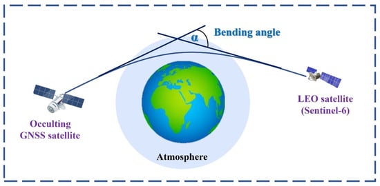
Figure 1.
A schematic of GNSS RO geometry.
In this study, four different techniques are discussed to determine the TPH from GNSS RO. The TPH was estimated from the lapse rate, cold point, N, and BA. By examining the temperature profile obtained from the processing of GNSS RO data, the inflection point in the temperature profile was defined as the lapse rate tropopause (LRT) based on the World Metrological Organization (WMO 1957 definition [35]. The LRT method is widely used because it is a simple and easy method to apply to the temperature profile generated from GNSS RO data or radiosondes [20,22,23,36].
Seidel et al. [7] estimated the global TPH from radiosonde data using the lapse rate tropopause method. Nishida et al. [17] determined the TPH from Global Positioning System (GPS)/Meteorology (MET) data using the LRT method. Zhran and Mousa [22] estimated the global TPH using the LRT method from Meteorological Operational Polar Satellite (MetOp) data. Liu et al. [23] identified the TPH from the FengYun 3 series C satellite (FY-3C) data using the LRT method. Schmidt et al. [21] determined the global TPH from the Challenging Minisatellite Payload (CHAMP) satellite data and the U.S.-Argentinian Satelite de Aplicaciones Cientificas-C (SAC-C) data using the LRT method. The lowest value in the temperature profile serves as the cold point tropopause (CPT) definition. The TPH, based on the CPT definition, is recommended for the investigation of the cross-tropopause flow of water vapor in the tropics [37]. Schmidt et al. [5] determined the TPH using both LRT and CPT definitions from the CHAMP satellite and discovered that the tropical LRT height fluctuated between 16.5 and 16.8 km, and that the CPT height across the tropics (10°N to 10°S) was longitudinally constant at 17.0 km. The CPT height is on average 400 m higher than the LRT height. Using 83 radiosondes launched in locations within the tropics (30°S to 30°N), Seidel et al. [38] found that the annual mean zonal mean CPT height was relatively constant across latitudes at ~16.9 km, and the annual mean zonal mean LRT height varied from ~16.5 km in the deep tropics to less than 16 km in the subtropics, implying a latitude-dependent separation between the two tropopauses of 500 m to 1 km.
For the GNSS RO data, estimating the TPH from the lapse rate requires some assumptions, such as dry air and a priori knowledge of the hydrostatic equation integration. Identifying the TPH from the BA is superior, such that there is no need for the hydrostatic equilibrium assumption. The BA is the primary core of the GNSS RO data. The BA can also be determined indirectly from radiosonde data and daily operational forecast data through the Abel transform inversion, which estimates the BA from N.
The N obtained from the Abelian transformation can be used for the identification of the TPH, and the obtained value is referred to as the TPHN. Xia et al. [39] detected the TPH using the atmospheric N from the Constellation Observing System for Meteorology, Ionosphere, and Climate (COSMIC) RO data. The covariance transform (CT) method described by Lewis [40] was used to estimate the TPH directly from the BA () to determine the transition in the , and the resulting TPH from this method is called the TPHα. Zhang et al. [24] identified the TPH based on the BA from COSMIC RO data using the CT method. Liu et al. [16] also determined the TPH based on the BA and the LRT using FY-3C and MetOp RO data. The TPH determined from the BA is a function of the impact parameter. To convert the impact parameter to the impact altitude above the geoid, the radius of curvature and geoid undulation values must be subtracted from the impact parameter.
This study aims to identify the TPH using different techniques according to the definition of WMO: LRT and CPT. In addition, this study aims to determine the TPH from the BA and N, which is considered an additional method developed specifically for use with the GNSS RO data based on the CT method. The analysis is performed on a new data source (Sentinel-6) that receives data in the open-loop tracking mode. Setinel-6 (hereafter S6) has a high circular inclination orbit (66°). S6 captures signals from the Global Positioning System (GPS) and Russia’s Global Navigation Satellite System (GLONASS), thereby increasing the number of obtained profiles. So far, to the best of our knowledge, the evaluation of the TPH using S6 data and different techniques has not been investigated.
This paper is structured as follows: data sources and methods, including the processing of the GNSS RO data from S6 for the identification of the TPH using different algorithms, are described in Section 2. Section 3 presents the analysis and discussion of the results. Finally, the conclusions of this study are presented in Section 4.
2. Data and Methods
2.1. GNSS RO Data
For the identification of the TPH from different algorithms, the GNSS RO data (atmPrf) from S6 were used in this study. The data used in this study covers the period from January 2022 to June 2022. From these data, the LRT and CTP heights, TPHN, and TPHα were estimated. Figure 2a shows an example of the distribution of the GNSS RO events on a selected day. The monthly distribution of the GNSS RO events by S6 in January 2022 is presented in Figure 2b. As shown in Figure 2, the GNSS RO distribution is almost uniform across the world. The massive amount of data from S6 significantly enhances the study of the tropopause. From the previous figures, it can be seen that S6 has a good spatial distribution over land and sea. All latitudinal zones were covered by observations, as shown in Figure 2. S6 can sense the atmosphere and study the dynamics of the tropopause globally.
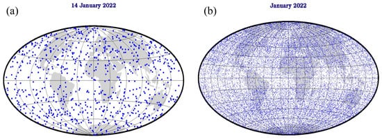
Figure 2.
Distribution of GNSS RO events from Sentinel-6 on 14 January 2022 (a) and in January 2022 (b).
Figure 3a illustrates the monthly RO profile from S6 from January 2022 to June 2022. During this period, there were approximately 154,279 GNSS RO profiles. In this study, the GNSS RO data retrieved from S6 were downloaded from https://rom-saf.eumetsat.int/pub/ntc/profs/sentinel6/atm/ (accessed on 30 September 2022). Temperature, N, and BA profiles were obtained from the processing of the GNSS RO data to identify the TPH using different algorithms.
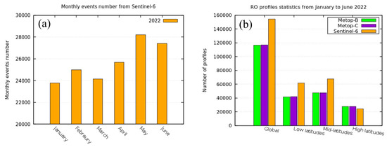
Figure 3.
Monthly RO profiles numbers from Sentinel-6 from January to June 2022 (a) and RO profiles statistics from MetOp-B, MetOp-C, and S6 for the global and latitudinal data sets from January to June 2022 (b).
The distribution of RO profiles from S6 is compared with the RO data from the MetOp Series (MetOp-B and MetOp-C) during the same study period. Figure 3b presents the RO profile statistics from MetOp-B, MetOp-C, and S6 according to the latitudinal distribution bands as follows: global (−90° to +90°), low (−30° to +30°), middle (±30° to ±60°), and high (±60° to ±90°) latitudes. As presented in Figure 3b, RO profiles from S6 are higher than RO profiles from MetOp-B and MetOp-C. As reported by Zhran [41], S6 provided more RO data than MetOp-B and MetOp-C because S6 receives GPS and GLONASS signals, unlike MetOp-B and MetOp-C, which receive only GPS signals. S6 provides higher data at low and mid latitudes compared to MetOp-B and MetOp-C.
The results of the TPH from S6 using different techniques were compared with the European Center for Medium-Range Weather Forecasts (ECMWF) daily operational forecasts, downloaded from https://rom-saf.eumetsat.int/pub/ntc/profs/sentinel6/bgo/ (accessed on 30 September 2022). The S6 satellite was used in this study as a new data source for the remote sensing of the atmosphere. The phase delay of the signal is determined by comparing the phase received by the LEO receiver to the known phase of the signal from the GNSS satellite, thereby creating an excess phase. The time derivative of the excess phase is the excess Doppler shift. Geometric optics retrievals on the excess Doppler shift and the satellite/receiver geometries were used to determine an accumulated BA [42]. After performing ionospheric corrections to the BA on L1 and L2, the neutral BA was retrieved. Statistical optimization is used for the initialization of the neutral BA at high altitudes and is necessary for noise reduction [43,44]. The sources of RO errors in the upper stratosphere include measurement noise, bending angle initialization for the Abel transform, and ionospheric residuals following the dual-frequency ionospheric correction [29].
By applying the inverse Abelian transformation, the BA is transformed into N using the spherical symmetry assumption [45]. As the refractive index is close to unity, N is preferred for studying the atmosphere [42]. The refractivity is defined as N = (n − 1) × 106. We calculated the temperature profile using hydrostatic equilibrium. By disregarding the existence of water vapor, the dry temperature may be obtained from refractivity data. This indicates that if the contribution of water vapor to the refractivity is negligible, as it usually is in the high troposphere and stratosphere, then the dry temperature is near the physical temperature.
In the ROPP, the pressure at 150 km is determined using the refractivity gradient at this height, ignoring the temperature gradient, in order to initiate the hydrostatic integration. The BA alone did not yield a temperature profile. Figure 4 illustrates the primary phases in the GNSS RO data processing in the ROPP.
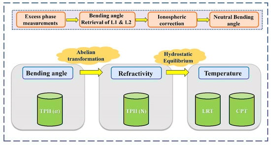
Figure 4.
Graphical abstract of the processing flow.
Zhran [41] validated the atmospheric profiles from S6 with MetOp-B, MetOp-C, and ECMWF Reanalysis v5 (ERA5) and found that, for the monthly zonal mean dry temperature, most of the standard deviation (STD) values from S6 are in the range of 2 to 4 K at heights of 10 to 35 km. In tropical regions, the STD is of greater significance than in polar zones below 10 km.
2.2. Methods of TPH Estimation
The WMO established the LRT definition as the lowest height at which the temperature lapse rate is less than 2 °C/km, and the average temperature lapse rate between this height and the level 2 km above it does not exceed 2 °C/km [35]. The CPT height is indicated by the lowest value in the temperature profile. To define the tropical tropopause, the CPT has become increasingly important because of the improved correlation between tropical tropopause features and convective processes, which are crucial to the stratosphere–troposphere interchange [46].
An example of a GNSS RO temperature profile at a specific location at night, indicated by the TPH computed from the LRT and CPT, is presented in Figure 5. As this graph illustrates, the CPT height was higher than the LRT height.
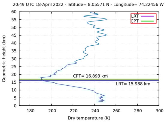
Figure 5.
TPH determination from LRT and CPT on the temperature profile.
The CT approach was applied to all BAs generated by S6 from January 2022 to June 2022 as well as N profiles. For comparison, the result of the TPHs generated based on the BA is converted to the geometric height instead of the impact parameter. For more details about the CT approach, refer to the study by Lewis [40].
Lewis [40] developed the CT approach used by the ROPP. The CT approach introduces the determination of the TPH based on the BA profiles without the need for any a priori information. The TPHα is the maximum CT of the logarithm of the BA, which is defined as follows [47]:
where and are the lower and upper limits of the data profile, respectively; a is the vertical scale involved in the calculation. is the width of the CT and was fixed at 25 km in the ROPP based on the result of some experimentation with a variety of occultation profiles. is the natural logarithm of the BA () at the impact parameter () normalized by as follows [47]:
For the identification of the TPHN, Equation (1) was used again, but now is the natural logarithm of the at height () normalized by 1000 N-units as follows:
Refractivity can be obtained from different sources; therefore, this algorithm can be applied to the N extracted from daily operational forecasts. The ROPP is used for the identification of the different TPHs from the profiles of temperature, refractivity, and bending angle. The altitude range in the tropopause that the different algorithms in the ROPP search for has the following lower bounds (TPH min) and higher bounds (TPH max) [16]:
where denotes the atmospheric profile’s latitude.
3. Results and Analysis
3.1. TPH from Various Algorithms
The distribution of the LRT height and latitude during the study period is shown in Figure 6. Figure 6 depicts that the LRT has its highest value at the equator and its lowest value at the poles. Additionally, Figure 6 also shows that the LRT height is dependent mainly on latitude and decreases with latitude in both the northern and southern hemispheres, which is consistent with the results published by Schmidt et al. [5]. As presented in Figure 6, there is a break between the upper and lower tropopauses around 20–30°N in January, February, and March. A similar asymmetry looks to be beginning to develop in the southern hemisphere in the June data. The LRT algorithm is globally applicable for identifying the TPH.
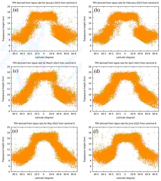
Figure 6.
Distribution of LRT height during the study period.
Figure 7 shows the analysis of the CPT height, which indicates that the CPT is only applicable in the tropics between 30°S and 30°N. Outside of the tropics, the cold point is not necessarily reflective of the tropopause, so the CPT tropopause is not calculated. It is not always possible to utilize the computed CPT since the cold point might occur at the tropopause or higher in the stratosphere. Additionally, at mid latitudes, the occurrence of double tropopauses also makes the interpretation more complicated. To ascertain how latitude relates to the CPT and LRT heights, the LRT is drawn in the tropics only from 30°S to 30°N alongside the same latitude band in Figure 7. The TPH based on the CPT is higher than that based on the LRT, which is consistent with the results published by Schmidt et al. [5]. The identification of the tropical tropopause is better represented by the CPT, where air convection is relatively uncomplicated. The CPT would be preferred for studies of the transport of water vapor across the tropical tropopause, as it represents the point in the vertical motion when an air parcel will encounter the lowest temperature.
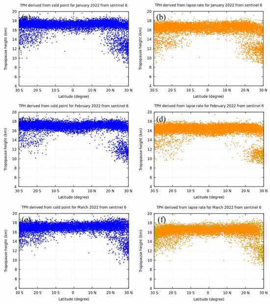
Figure 7.
Distribution of TPH based on CPT and LRT sliced at the same location of solved CPT from January to March 2022.
The TPH derived from N during the study period is depicted in Figure 8. The TPH pattern has two sub-patterns. One follows the LRT height, which is highest at the equator and lowest at the poles, and the other one traces a smooth curve indicating the highest TPH, which indicates that this is a signal of a double tropopause. As shown in Figure 8, there was a double layer in the TPH distribution outside the tropics. In the sub-tropical region, there are often tropopause folds, leading to a double-tropopause structure. This means that the algorithms are unstable in that small changes can lead the algorithm to switch between the diagnosis of either the higher or lower temperature minimum. The change between these two minima can lead to large differences in the algorithms and would be a source of substantial challenge and perhaps interest.
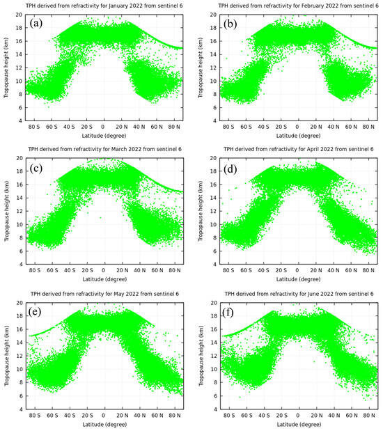
Figure 8.
Distribution of TPH based on refractivity during the study period.
Figure 9 illustrates the TPH distribution derived from the BA during the study period. The TPHα follows the same pattern as the LRT height, where the maximum value occurs at the equator, and the minimum value occurs at the poles. In general, the TPH patterns from different algorithms are symmetric about the equator on a broad scale.
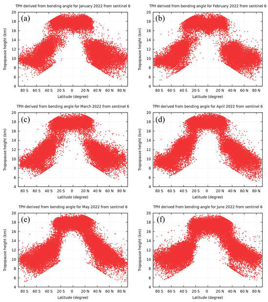
Figure 9.
Distribution of TPH based on BA during the study period.
A repeated measures one-way analysis of variance (ANOVA) at a 95% confidence interval was used to analyze the data. The results show a p-value < 0.0001, which means that the difference between the LRT height, CPT height, TPH derived from N, and TPH derived from BA is significant.
3.2. Comparison of LRT Heights
TPHs based on the CPT, N, and BA were compared with TPHs based on the LRT. In this comparison, the LRT height was used as the reference because it is applicable for all latitude ranges, while the CPT is spatially limited. To analyze the difference between the LRT and CPT in detail, the latitude bands were divided by ten degrees for the northern and southern hemispheres. The LRT and CPT heights were estimated from the temperature profiles obtained from the GNSS RO data processing.
Figure 10 shows the latitudinal distribution of the mean difference (MD) and correlation between the LRT and CPT heights. The MDs between the LRT and CPT heights (CPT-LRT) are examined with latitude in Table 1 because the TPH is highly correlated with latitude. Table 1 shows that the LRT and CPT heights are more consistent near the equator and at lower latitudes. Table 1 also shows that the CPT height was higher than the LRT height. As shown in Table 1, the MD at and near the equator had its lowest values for both the northern and southern hemispheres. The increase in latitude increased the MD between the LRT and CPT heights, which ensured that the LRT and CPT were more consistent at and near the equator.
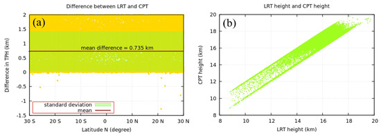
Figure 10.
Mean difference (CPT-LRT) (a) and correlation between LRT and CPT heights during the study period (b).

Table 1.
Mean difference between LRT and CPT heights during the study period.
We compared the results of TPHs based on N with TPHs based on the lapse rate. The mean bias between the LRT height and the TPH based on N for different latitude bands is shown in Figure 11. The MD is estimated for each ten-degree latitude band in the Northern Hemisphere. As shown in Figure 11, the MD increases with latitude up to 40°N and then decreases until 60°N. The lowest MD is 0.267 km at the 50–60°N zone, while the highest MD is 1.963 km at the 30–40°N zone. Figure 11b also shows that the largest differences occur in the subtropical zone (30–40°N), and there is also a large difference in the polar region (80–90°N) as presented in Figure 11a, which illustrates that TPH based on N is not very reliable for these latitude zones.
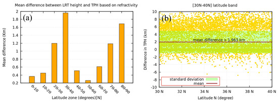
Figure 11.
Difference between LRT height and TPH based on refractivity for different latitude bands from 0 to 90°N every 10 degrees (a) showing latitude zone of maximum difference (b).
To analyze the difference between the LRT height and the TPH based on the BA, the latitude bands in the Northern Hemisphere were divided into nine zones, with each zone consisting of ten degrees. The MD and the standard deviation (STD) of the differences were estimated for each zone. As shown in Figure 12a, the largest MD was 1.12 km from the equator to 20°N and the largest MD between the LRT height and the TPH based on the BA is presented in Figure 12b. In general, in the latitude band of 30–40°N, the TPH based on BA exhibited the maximum variation as presented in Figure 12a.

Figure 12.
Difference between LRT height and TPH based on BA for different latitude bands from 0 to 90°N every 10 degrees (a) showing latitude zone of maximum difference (b).
3.3. Determination of the Zonal Mean
Next, the zonal mean of the TPH during the study period was determined using different algorithms. The results were gridded into a 5°-latitude band. For each grid, the zonal mean of the TPH from different approaches was estimated. A comparison between the zonal mean LRT and CPT heights is shown in Figure 13 for different latitude bands. As shown in Figure 13, the zonal mean CPT height was always higher than the zonal mean LRT height. As shown in Figure 13, the overall zonal MD is approximately 0.5 km at and near the equator and approximately 1 km at a latitude of 30°.
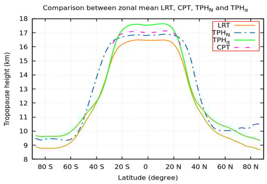
Figure 13.
Zonal mean LRT height, CPT height, TPHN, and TPHα during the study period.
Comparisons between the zonal mean LRT height, TPHN, and TPHα are shown in Figure 13. It is clear from Figure 13 that the LRT height is always smaller than the TPHN and TPHα. Between 20°S and 20°N, the TPHα is greater than the TPHN. From a latitude of 20° to approximately 45°, the TPHα is lower than the TPHN. Figure 13 clearly illustrates that the TPH from different techniques decreases with latitude for both the northern and southern hemispheres. As illustrated in Figure 13, the TPHα is greater than the LRT height, which is in excellent agreement with the results of Lewis (2009). This is due to the fact that the LRT criteria identifies the lowest possible TPH, while the BA method determines the most significant transition. There is good agreement between the LRT height and the TPH based on the BA between the latitudes of 30° to 40°, and through this band of latitude, there is a sharp decrease in the TPH values. The maximum difference between the LRT height and the TPH based on the BA is at and near the equator and from 40° towards the poles.
In general, as shown in the previous figure, the TPHα had the largest value followed by the TPHN, and the LRT had the lowest value of the TPH at and near the equator. The maximum TPH occurred in the equatorial region, whereas the minimum TPH occurred at the poles. In the equatorial region, the maximum TPH results from the TPHα (approximately 17.5 km), and at the poles, the minimum TPH results from the LRT (approximately 9 km) during the study period. Zhang et al. [24] found that the maximum TPH estimated from COSMIC data is found at the equator, which varies around 17 ± 0.5 km, and the minimum TPH is found at the North Pole, which fluctuates around 9.2 ± 1 km. Our results agree well with the results of Zhang et al. [24]. The previous figure shows that the slope of the TPH is steep in mid-latitude bands. For all the TPH methods, the strongest gradients were found between 20° and 40° in both hemispheres, while the TPH was constant between the equator and 20° in both hemispheres.
As an example, the STD of the zonal means for the different algorithms used for the identification of the TPH in June 2022 is presented in Figure 14. From Figure 14, it can be observed that the STD of the zonal mean is the lowest at the equator, increases with latitude until 40°, then decreases again. The STD of the zonal mean was generally symmetric about the equator. From Figure 14, it can be further seen that the CPT and LRT height provide the minimum STD, and the TPH based on N presents the maximum STD. Figure 14 clearly shows that, generally, the STD of the TPHα is higher than the STD of the LRT height, except at the poles, due to the fact that in the case of multiple tropopause transitions occurring in a profile, the bending angle transition at the upper layers is greater than at the lowest tropopause.
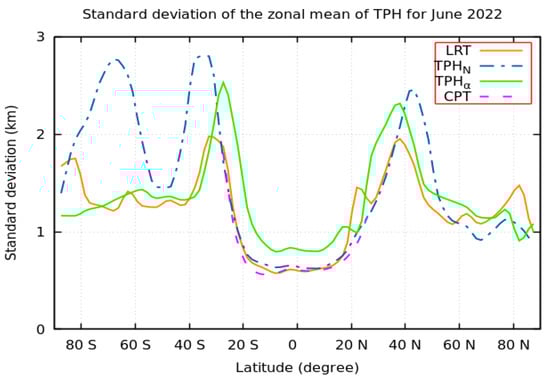
Figure 14.
The STD of the zonal means for different algorithms for identification of TPH for June 2022.
Figure 15 depicts the zonal mean for the LRT temperature and the CPT temperature during the study period in the low latitude band. As shown in Figure 15, the LRT temperature is higher than the CPT temperature with a mean difference of 1.1 k, and the correlation coefficient between them is 0.9998. Remarkably, both the LRT temperature and the CPT temperature increase with latitude, and there is symmetry in the northern and southern hemispheres for the LRT temperature and the CPT temperature. These results are in good agreement with the results published by Schmidt et al. [5]. A t-test was conducted at a 95% confidence interval to check if there was a significant difference between the LRT and CPT temperatures. The results show a p-value < 0.0001, which means that the difference between the LRT and CPT temperatures is significant.
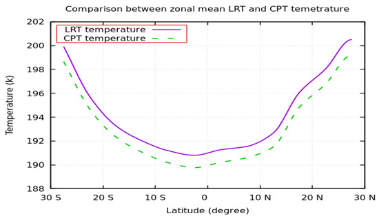
Figure 15.
Zonal mean LRT temperature and CPT temperature during the study period.
3.4. Determination of the Monthly Mean
Next, the TPH monthly mean variations and standard error determined by different algorithms during the study period were discussed. The monthly mean and standard error of the LRT height, CPT height, TPH based on N, and TPH based on the BA in different latitude bands are presented in Figure 16. From Figure 16, we can see that the TPH is generally high at low latitudes and low at high latitudes. As observed in Figure 16a, at low latitudes (−30° to +30°), the LRT height is the lowest TPH, while the TPH based on the BA is the highest TPH based on the monthly mean. These results agree well with Xia et al. [39]. Figure 16a highlights that the CPT height is greater than the LRT height, and the TPH based on the BA is higher than the TPH based on N at low latitudes. As presented in Figure 16a, there is a little variation in the TPH based on N at low latitudes.
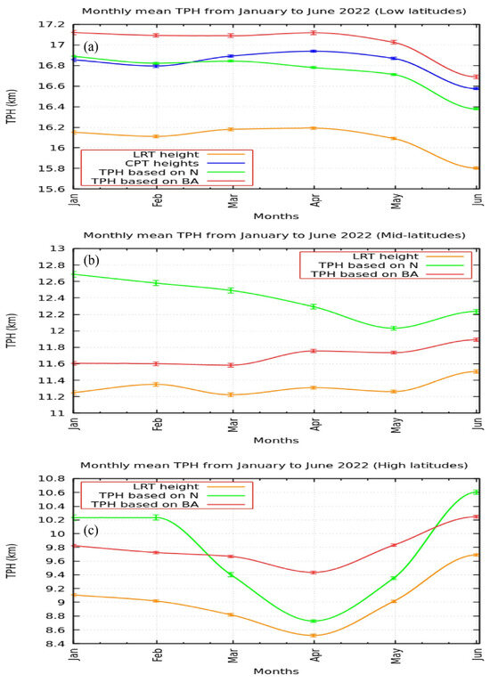
Figure 16.
The monthly mean variation of TPH computed by different algorithms with the standard error from January to June 2022 in different latitude bands.
At the mid latitudes (±30° to ±60°), the TPH based on N is the highest, while the LRT height is the lowest TPH, as shown in Figure 16b; unlike at low latitudes, at the mid latitudes, the TPH based on N is higher than the TPH based on the BA. At high altitudes (±60° to ±90°), there is no constant trend for the TPH based on N and the TPH based on the BA, as illustrated in Figure 16c. Generally, the LRT height is the lowest TPH at all latitude bands, as shown in Figure 16. It is worth remarking that the LRT height curve is almost parallel to the TPH based on the BA at all latitude bands, and this indicates that the LRT height and TPHα detect the same TPH variation trend.
The monthly mean variation of the LRT and CPT temperatures with the standard error from January to June 2022 at the low latitude band is highlighted in Figure 17. Interestingly, the monthly mean LRT temperature is higher than the monthly mean CPT temperature, as highlighted in Figure 17. It can be seen from Figure 17 that the LRT and CPT temperatures have the same pattern. The mean difference between the monthly mean LRT temperature and the monthly mean CPT temperature is 1.18 k, and the correlation coefficient between them is 0.98.
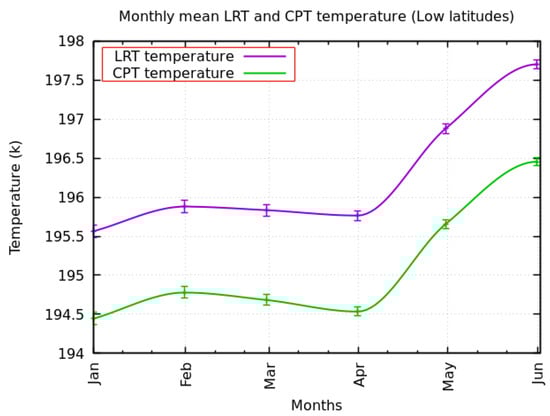
Figure 17.
The monthly mean variation of LRT and CPT temperature with the standard error from January to June 2022 at the low latitude band.
3.5. Evaluation of TPH with ECMWF
In this study, we validated the results of the TPH derived from the different algorithms with an external data source. The ECMWF operational forecast is used as a reference for the comparison in June 2022. The TPH from different approaches were estimated from the co-located ECMWF profiles. A comparison between the CPT heights estimated from GNSS RO and the ECMWF model in June 2022 is illustrated in Figure 18. As illustrated in Figure 18, there was a strong correlation between the zonal mean CPT height estimated from GNSS RO and the values determined from the ECMWF model of approximately 0.9996.
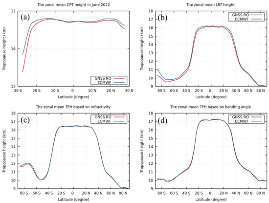
Figure 18.
The comparison between zonal mean CPT height (a), LRT height (b), TPHN (c), and TPHα (d) from GNSS RO and ECMWF model in June 2022.
Figure 18 also shows the comparison between the zonal mean LRT height determined from GNSS RO and the ECMWF model in June 2022. Figure 18 also illustrates that the two approaches have a high degree of agreement, with a correlation value of 0.9998. The validations for the TPH based on N and the TPH based on the BA are also illustrated in Figure 18. Figure 18 shows that there is a high correlation of approximately 0.9997 between the zonal mean TPHN values calculated from the ECMWF model and those estimated from GNSS RO. Figure 18 demonstrates that there is a strong correlation between the zonal mean TPHα values obtained from the ECMWF model and those derived using GNSS RO, with a coefficient of approximately 0.9997.
The zonal mean bias (GNSS RO-ECMWF) for the LRT height, CPT height, TPHN, and TPHα derived from GNSS RO, and their values estimated from the ECMWF model in June 2022, are depicted in Figure 19. As shown in Figure 19, the LRT yielded the maximum zonal bias. The mean zonal values of the difference were −185 m for the LRT height, −6 m for the TPHN, and 0.09 m for the TPHα. These results clearly show that the TPH derived from the BA introduces the least mean zonal bias, followed by N, because the temperature is derived from N based on assumptions such as hydrostatic equilibrium, and N is determined from the BA based on the spherical symmetry assumption. No assumptions were required for determining the TPH from the BA except for the spherical symmetry assumption, so it is a novel method for determining the TPH. Table 2 lists the zonal mean bias of the LRT height in different months in 2022. Table 2 ensures that GNSS RO underestimates the LRT height compared to the ECMWF operational forecast.
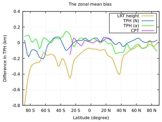
Figure 19.
The zonal mean bias (GNSS RO—ECMWF) in June 2022.
Table 2.
The zonal mean bias (GNSS RO—ECMWF) in LRT height during the study period.
From the above discussion, it can be seen that the LRT height leads to maximum zonal bias and the TPHα yields minimum zonal bias. Additionally, we analyzed the LRT height and the TPHα estimated from GNSS RO and the ECMWF model in the tropical, subtropical, and polar regions in the Northern Hemisphere, as highlighted in Figure 20. The results in Figure 20 were gridded into a 5°-latitude band.
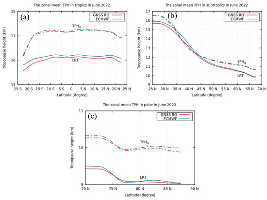
Figure 20.
The comparison between zonal mean LRT height and TPHα from GNSS RO and the ECMWF model in June 2022 in tropical (a), subtropical (b), and polar regions (c).
Figure 20 shows that GNSS RO underestimates the LRT height compared to the ECMWF model in tropical, subtropical, and polar regions in the Northern Hemisphere, while GNSS RO overestimates the TPHα compared to the ECMWF model in tropical regions. Interestingly, in subtropical regions, the TPHα computed from GNSS RO and ECMWF model are almost identical. Notably, GNSS RO underestimates the TPHα compared to the ECMWF model in the polar regions. Figure 20 also highlights that the TPHα is generally greater than the LRT height, while at the latitudes of 35° to 45°, the LRT height and the TPH based on the BA are nearly identical.
The LRT height profiles in the tropical, subtropical, and polar regions in the Northern Hemisphere, estimated from GNSS RO and the ECMWF model, are presented in Figure 21. Figure 21 ensures that GNSS RO underestimates the LRT height compared to the the ECMWF model in tropical, subtropical, and polar regions in the Northern Hemisphere, as illustrated in different profiles. These profiles also illustrate that the TPH mainly decreases with latitude.

Figure 21.
LRT height profiles in the tropical (a), subtropical (b), and polar regions (c) in the Northern Hemisphere, estimated from GNSS RO and the ECMWF model.
In the future, more radio occultation data from GPS, BDS, Galileo and GLONASS will provide more atmospheric parameter profiles [48,49,50], which will further improve the accuracy and resolution of TPH estimation. More variation characteristics of the TPH will be studied and revealed.
4. Conclusions
The identification of the TPH is important for climate studies. Different techniques for identifying the TPH using Sentinel-6 data, including identifying the TPH based on the LRT and CPT, based on N, and based on the BA, were investigated. The results show that GNSS RO can identify the TPH using four different algorithms. The LRT is globally applicable, whereas the CPT is valid only in the tropics. The CPT is a better indicator of the tropical tropopause. Because there are various methods for obtaining N, the TPH based on the N algorithm can be used with any source that offers this property. The global TPH can be calculated directly from the BA using GNSS RO rather than radiosonde clustering at specific locations. The TPH can be identified directly from the BA instead of temperature profiles, without the need for any a priori knowledge of hydrostatic equation integration.
The equatorial region had the highest TPH, whereas the poles had the lowest TPH. At and near the equator, the TPHα is often the highest value, followed by the TPHN; the LRT height has the lowest value of TPH. The TPHα (approximately 17.5 km) produced the highest TPH in the equatorial region, and the LRT produced the lowest TPH near the poles (approximately 9 km) during the study period. The TPHs from different approaches estimated from ECMWF daily operational forecasts are in very good agreement with those estimated from GNSS RO, with a correlation coefficient of 0.999. The mean zonal difference between GNSS RO and ECMWF model was the lowest for the TPH based on the BA, and highest for the LRT height. In tropical, subtropical, and polar areas, GNSS RO underestimates the LRT height in comparison with the ECMWF model, whereas in tropical regions, the GNSS RO overestimates the TPHα.
In conclusion, GNSS RO is an effective remote sensing tool for identifying the tropopause height and is a diagnostic tool for studying the atmosphere because of its high resolution, high precision, and good spatial and temporal coverage. GNSS RO alone offers four different algorithms for imaging the spatiotemporal TPH with global coverage. According to our results, the TPHα is the most effective method for identifying the TPH without the need for any a priori information, unlike the other methods. This study offers a helpful foundation for future research on the long-term fluctuations in tropopause height.
Author Contributions
Conceptualization, M.Z. and A.M.; methodology, M.Z. and A.M.; software, M.Z.; validation, M.Z.; formal analysis, M.Z.; investigation, M.Z.; resources, M.Z.; data curation, M.Z.; writing—original draft preparation, M.Z.; writing—review and editing, M.Z., A.M., F.A. and S.J.; visualization, M.Z. All authors have read and agreed to the published version of the manuscript.
Funding
This research was funded by Abdullah Alrushaid Chair for Earth Science Remote Sensing Research at King Saud University, Riyadh, Saudi Arabia.
Data Availability Statement
GNSS RO data were downloaded from www.romsaf.org (accessed on 30 September 2022).
Acknowledgments
The authors extend their appreciation to Abdullah Alrushaid Chair for Earth Science Remote Sensing Research for funding.
Conflicts of Interest
The authors declare no conflict of interest.
References
- Johnston, B.; Xie, F. Characterizing Extratropical Tropopause Bimodality and Its Relationship to the Occurrence of Double Tropopauses Using COSMIC GPS Radio Occultation Observations. Remote Sens. 2020, 12, 1109. [Google Scholar] [CrossRef]
- Johnston, B.R.; Xie, F.; Liu, C. The Effects of Deep Convection on Regional Temperature Structure in the Tropical Upper Troposphere and Lower Stratosphere. J. Geophys. Res. Atmos. 2018, 123, 1585–1603. [Google Scholar] [CrossRef]
- Munchak, L.A.; Pan, L.L. Separation of the Lapse Rate and the Cold Point Tropopauses in the Tropics and the Resulting Impact on Cloud Top-Tropopause Relationships. J. Geophys. Res. 2014, 119, 7963–7978. [Google Scholar] [CrossRef]
- Xu, X.; Luo, J.; Zhang, K. An Analysis of the Structure and Variation of the Tropopause over China with GPS Radio Occultation Data. J. Navig. 2011, 64, S103–S111. [Google Scholar] [CrossRef]
- Schmidt, T.; Wickert, J.; Beyerle, G.; Reigber, C. Tropical Tropopause Parameters Derived from GPS Radio Occultation Measurements with CHAMP. J. Geophys. Res. Atmos. 2004, 109. [Google Scholar] [CrossRef]
- Santer, B.D.; Sausen, R.; Wigley, T.M.L.; Boyle, J.S.; AchutaRao, K.; Doutriaux, C.; Hansen, J.E.; Meehl, G.A.; Roeckner, E.; Ruedy, R.; et al. Behavior of Tropopause Height and Atmospheric Temperature in Models, Reanalyses, and Observations: Decadal Changes. J. Geophys. Res. Atmos. 2003, 108, ACL-1. [Google Scholar] [CrossRef]
- Seidel, D.J.; Randel, W.J. Variability and Trends in the Global Tropopause Estimated from Radiosonde Data. J. Geophys. Res. Atmos. 2006, 111. [Google Scholar] [CrossRef]
- Santer, B.D.; Wehner, M.F.; Wigley, T.M.L.; Sausen, R.; Meehl, G.A.; Taylor, K.E.; Ammann, C.; Arblaster, J.; Washington, W.M.; Boyle, J.S.; et al. Contributions of Anthropogenic and Natural Forcing to Recent Tropopause Height Changes. Science 2003, 301, 479–483. [Google Scholar] [CrossRef]
- Sausen, R.; Santer, B.D. Use of Changes in Tropopause Height to Detect Human Influences on Climate. Meteorol. Z. 2003, 12, 131–136. [Google Scholar] [CrossRef]
- Meng, L.; Liu, J.; Tarasick, D.W.; Li, Y. Biases of Global Tropopause Altitude Products in Reanalyses and Implications for Estimates of Tropospheric Column Ozone. Atmosphere 2021, 12, 417. [Google Scholar] [CrossRef]
- Wang, C.-Y.; Xie, S.-P.; Liu, Q.; Zheng, X.-T. Global Influence of Tropical Pacific Variability with Implications for Global Warming Slowdown. J. Clim. 2017, 30, 2679–2695. [Google Scholar] [CrossRef]
- Di Noia, A.; Sellitto, P.; Del Frate, F.; De Laat, J. Global Tropospheric Ozone Column Retrievals from OMI Data by Means of Neural Networks. Atmos. Meas. Tech. 2013, 6, 895–915. [Google Scholar] [CrossRef]
- Schmidt, T.; Beyerle, G.; Heise, S.; Wickert, J.; Rothacher, M. A Climatology a Multiple Tropauses Derived from GPS Radio Occultations with CHAMP and SAC-C. Geophys. Res. Lett. 2006, 33, 6110. [Google Scholar] [CrossRef]
- Feng, S.; Fu, Y.; Xiao, Q. Trends in the Global Tropopause Thickness Revealed by Radiosondes. Geophys. Res. Lett. 2012, 39. [Google Scholar] [CrossRef]
- Mateus, P.; Mendes, V.B.; Pires, C.A.L. Global Empirical Models for Tropopause Height Determination. Remote Sens. 2022, 14, 4303. [Google Scholar] [CrossRef]
- Liu, Z.; Sun, Y.; Bai, W.; Xia, J.; Tan, G.; Cheng, C.; Du, Q.; Wang, X.; Zhao, D.; Tian, Y.; et al. Comparison of RO Tropopause Height Based on Different Tropopause Determination Methods. Adv. Space Res. 2021, 67, 845–857. [Google Scholar] [CrossRef]
- Nishida, M.; Shimizu, A.; Tsuda, T.; Rocken, C.; Ware, R.H. Seasonal and Longitudinal Variations in the Tropical Tropopause Observed with the GPS Occultation Technique (GPS/MET). J. Meteorol. Soc. Japan Ser II 2000, 78, 691–700. [Google Scholar] [CrossRef]
- Zali, R.M.; Mandeep, J.S. Tropopause Estimation from GPS-RO Space-Based by Using Covariance Linear Regression Technique. J. Commun. 2022, 17, 150–155. [Google Scholar] [CrossRef]
- Narayana Rao, D.; Venkat Ratnam, M.; Krishna Murthy, B.V.; Jagannadha Rao, V.V.M.; Kumar Mehta, S.; Nath, D.; Ghouse Basha, S. Identification of Tropopause Using Bending Angle Profile from GPS Radio Occultation (RO): A Radio Tropopause. Geophys. Res. Lett. 2007, 34, L15809. [Google Scholar] [CrossRef]
- Schmidt, T.; Wickert, J.; Beyerle, G.; Heise, S. Global Tropopause Height Trends Estimated from GPS Radio Occultation Data. Geophys. Res. Lett. 2008, 35, L11806. [Google Scholar] [CrossRef]
- Schmidt, T.; Heise, S.; Wickert, J.; Beyerle, G.; Reigber, C. GPS Radio Occultation with CHAMP and SAC-C: Global Monitoring of Thermal Tropopause Parameters. Atmos. Chem. Phys. 2005, 5, 1473–1488. [Google Scholar] [CrossRef]
- Zhran, M.; Mousa, A. Global Tropopause Height Determination Using GNSS Radio Occultation. Egypt. J. Remote Sens. Space Sci. 2023, 26, 317–331. [Google Scholar] [CrossRef]
- Liu, Z.; Sun, Y.; Bai, W.; Xia, J.; Tan, G.; Cheng, C.; Du, Q.; Wang, X.; Zhao, D.; Tian, Y.; et al. Validation of Preliminary Results of Thermal Tropopause Derived from FY-3C GNOS Data. Remote Sens. 2019, 11, 1139. [Google Scholar] [CrossRef]
- Zhang, X.; Gao, P.; Xu, X. Variations of the Tropopause over Different Latitude Bands Observed Using COSMIC Radio Occultation Bending Angles. IEEE Trans. Geosci. Remote Sens. 2014, 52, 2339–2349. [Google Scholar] [CrossRef]
- Vespe, F.; Pacione, R.; Rosciano, E. A Novel Tool for the Determination of Tropopause Heights by Using GNSS Radio Occultation Data. Atmos. Clim. Sci. 2017, 7, 301–313. [Google Scholar] [CrossRef][Green Version]
- Anthes, R.A. Exploring Earth’s Atmosphere with Radio Occultation: Contributions to Weather, Climate and Space Weather. Atmos. Meas. Tech. 2011, 4, 1077–1103. [Google Scholar] [CrossRef]
- Steiner, A.K.; Lackner, B.C.; Ladstdter, F.; Scherllin-Pirscher, B.; Foelsche, U.; Kirchengast, G. GPS Radio Occultation for Climate Monitoring and Change Detection. Radio Sci. 2011, 46, 1–17. [Google Scholar] [CrossRef]
- Wang, W.; Shangguan, M.; Tian, W.; Schmidt, T.; Ding, A. Large Uncertainties in Estimation of Tropical Tropopause Temperature Variabilities Due to Model Vertical Resolution. Geophys. Res. Lett. 2019, 46, 10043–10052. [Google Scholar] [CrossRef]
- Kursinski, E.R.; Hajj, G.A.; Schofield, J.T.; Linfield, R.P.; Hardy, K.R. Observing Earth’s Atmosphere with Radio Occultation Measurements Using the Global Positioning System. J. Geophys. Res. Atmos. 1997, 102, 23429–23465. [Google Scholar] [CrossRef]
- Gorbunov, M.E.; Benzon, H.H.; Jensen, A.S.; Lohmann, M.S.; Nielsen, A.S. Comparative Analysis of Radio Occultation Processing Approaches Based on Fourier Integral Operators. Radio Sci. 2004, 39, 1–11. [Google Scholar] [CrossRef]
- Gorbunov, M.E.; Shmakov, A.V.; Leroy, S.S.; Lauritsen, K.B. COSMIC Radio Occultation Processing: Cross-Center Comparison and Validation. J. Atmos. Ocean. Technol. 2011, 28, 737–751. [Google Scholar] [CrossRef]
- Syndergaard, S. Algorithm Theoretical Baseline Document: Level 1B Bending Angles. 2020. Available online: https://rom-saf.eumetsat.int/product_documents/romsaf_atbd_ba.pdf (accessed on 30 September 2022).
- Wickert, J.; Reigber, C.; Beyerle, G.; König, R.; Marquardt, C.; Schmidt, T.; Grunwaldt, L.; Galas, R.; Meehan, T.K.; Melbourne, W.G.; et al. Atmosphere Sounding by GPS Radio Occultation: First Results from CHAMP. Geophys. Res. Lett. 2001, 28, 3263–3266. [Google Scholar] [CrossRef]
- Zhran, M.; Mousa, A. Planetary Boundary Layer Height Retrieval Using GNSS Radio Occultation over Egypt. Egypt. J. Remote Sens. Space Sci. 2022, 25, 551–559. [Google Scholar] [CrossRef]
- WMO. Atmospheric Ozone 1985: Global Ozone Research and Monitoring Report; World Meteorological Organization (WMO): Geneva, Switzerland, 1986. [Google Scholar]
- Li, W.; Yuan, Y.B.; Chai, Y.J.; Liou, Y.A.; Ou, J.K.; Zhong, S. ming Characteristics of the Global Thermal Tropopause Derived from Multiple Radio Occultation Measurements. Atmos. Res. 2017, 185, 142–157. [Google Scholar] [CrossRef]
- Han, T.T.; Ping, J.S.; Zhang, S.J. Global Features and Trends of the Tropopause Derived from GPS/CHAMP RO Data. Sci. China Phys. Mech. Astron. 2011, 54, 365–374. [Google Scholar] [CrossRef]
- Seidel, D.J.; Ross, R.J.; Angell, J.K.; Reid, G.C. Climatological Characteristics of the Tropical Tropopause as Revealed by Radiosondes. J. Geophys. Res. Atmos. 2001, 106, 7857–7878. [Google Scholar] [CrossRef]
- Xia, P.; Shan, Y.; Ye, S.; Jiang, W. Identification of Tropopause Height with Atmospheric Refractivity. J. Atmos. Sci. 2021, 78, 3–16. [Google Scholar] [CrossRef]
- Lewis, H.W. A Robust Method for Tropopause Altitude Identification Using GPS Radio Occultation Data. Geophys. Res. Lett. 2009, 36, L12808. [Google Scholar] [CrossRef]
- Zhran, M. An Evaluation of GNSS Radio Occultation Atmospheric Profiles from Sentinel-6. Egypt. J. Remote Sens. Space Sci. 2023, 26, 654–665. [Google Scholar] [CrossRef]
- Kursinski, E.R.; Hajj, G.A.; Leroy, S.S.; Herman, B. The GPS Radio Occultation Technique. Terr. Atmos. Ocean. Sci. 2000, 11, 53–114. [Google Scholar] [CrossRef]
- Healy, S.B. Annales Geophysicae Smoothing Radio Occultation Bending Angles above 40 Km; European Geophysical Society: Munich, Germany, 2001; Volume 19, pp. 459–468. [Google Scholar] [CrossRef][Green Version]
- Gobiet, A.; Kirchengast, G.; Manney, G.L.; Borsche, M.; Retscher, C.; Stiller, G. Atmospheric Chemistry and Physics Retrieval of Temperature Profiles from CHAMP for Climate Monitoring: Intercomparison with Envisat MIPAS and GOMOS and Different Atmospheric Analyses. Atmos. Chem. Phys. 2007, 7, 3519–3536. [Google Scholar] [CrossRef]
- Fjeldbo, G.; Kliore, A.J.; Eshleman, R. The Neutral Atmosphere of Venus as Studied with the Mariner V Radio Occultation Experiments. Astron. J. 1971, 76, 123. [Google Scholar] [CrossRef]
- Highwood, E.J.; Hoskins, B.J. The Tropical Tropopause. Q. J. R. Meteorol. Soc. 1998, 124, 1579–1604. [Google Scholar] [CrossRef]
- Jin, S.G. (Ed.) The Radio Occultation Processing Package (ROPP) Applications Module User Guide ROPP APPS User Guide, 2021; Global Navigation Satellite Systems: Signal, Theory and Applications; InTech-Publisher: Rijeka, Croatia, 2021; Volume 49, p. 426. [Google Scholar]
- Jin, S.G.; Han, L.; Cho, J. Lower atmospheric anomalies following the 2008 Wenchuan Earthquake observed by GPS measurements. J. Atmos. Sol.-Terr. Phys. 2011, 73, 810–814. [Google Scholar] [CrossRef]
- Jin, S.; Wang, Q.; Dardanelli, G. A review on multi-GNSS for Earth observation and emerging applications. Remote Sens. 2022, 14, 3930. [Google Scholar] [CrossRef]
- Jin, S.G.; Gao, C.; Li, J. Atmospheric sounding from FY-3C GPS radio occultation observations: First results and validation. Adv. Meteorol. 2019, 2019, 4780143. [Google Scholar] [CrossRef]
Disclaimer/Publisher’s Note: The statements, opinions and data contained in all publications are solely those of the individual author(s) and contributor(s) and not of MDPI and/or the editor(s). MDPI and/or the editor(s) disclaim responsibility for any injury to people or property resulting from any ideas, methods, instructions or products referred to in the content. |
© 2023 by the authors. Licensee MDPI, Basel, Switzerland. This article is an open access article distributed under the terms and conditions of the Creative Commons Attribution (CC BY) license (https://creativecommons.org/licenses/by/4.0/).