3D LiDAR Multi-Object Tracking with Short-Term and Long-Term Multi-Level Associations

Abstract

LiDAR-based Multi-Object Tracking (MOT) is a critical technology employed in various autonomous systems, including self-driving vehicles and autonomous delivery robots. In this paper, a novel LiDAR-based 3D MOT approach is introduced. The proposed method was built upon the Tracking-by-Detection (TbD) paradigm and incorporated multi-level associations that exploit an object’s short-term and long-term relationships with the existing tracks. Specifically, the short-term association leverages the fact that objects do not move much between consecutive frames. In contrast, the long-term association assesses the degree to which a long-term trajectory aligns with current detections. The evaluation of the matching between the current detection and the maintained trajectory was performed using a Graph Convolutional Network (GCN). Furthermore, an inactive track was maintained to address the issue of incorrect ID switching for objects that have been occluded for an extended period. The proposed method was evaluated on the KITTI benchmark MOT tracking dataset and achieved a Higher-Order Tracking Accuracy (HOTA) of 75.65%, marking a 5.66% improvement over the benchmark method AB3DMOT, while also accomplishing the number of ID switches of 39, 74 less than AB3DMOT. These results confirmed the effectiveness of the proposed approach in diverse road environments.

1. Introduction

Tracking multiple objects in urban environments such as city roads or highways plays a vital role in preventing potential traffic accidents and ensuring safe autonomous driving. Multi-Object Tracking (MOT) can be conducted using various sensors such as LiDAR [1,2,3,4], cameras [5,6,7], or a fusion of multiple sensors [8,9,10]. Over MOT using other sensors, LiDAR-based MOT has the following strengths: (1) LiDAR-based MOT can track objects’ positions more accurately than other sensors due to its ability to measure distances accurately. (2) LiDAR is less affected by environmental conditions such as lighting, weather (e.g., rain, fog), and time of day compared to other sensors. This makes it more reliable in adverse conditions. These strengths of LiDAR-based MOT have led to a great deal of research regarding the topic [11,12]. The majority of LiDAR-based MOT methods involve detecting objects in the current frame and associating them with existing tracks, namely taking Tracking-by-Detection (TbD) approaches. The TbD approaches in LiDAR-based MOT are quite effective in many cases, but sometimes suffer from difficulties in handling missed objects (due to detector or sensor failures) and occluded objects, as they significantly impact tracking performance.

Some of the LiDAR-based MOT methods have tackled the problem by using short-term relations between the current detection and the existing tracks. Specifically, they measure a distance (or the similarity) between the current detection and the new predictions predicted from the past few frames of the existing tracks in terms of the Intersection over Union (IoU) [1,4,6,7,9,10] or distance [2,3,8] and associate the current detection and the existing tracks based on the distance. While these methods that perform short-term association generally perform well, they sometimes suffer from the possibilities of misassociation between the detection and the track or the failure in maintaining a track, resulting in an ID switching problem. Figure 1 shows the typical example of incorrect ID switching. The vehicle enclosed within the yellow box in Figure 1a starts to be occluded by another vehicle, which turns left. In the next step, the vehicle inside the yellow box is completely occluded by the left-turning vehicle and is not detected as all, as shown in Figure 1b. After the left-turning vehicle has passed, the occluded vehicle that was inside the yellow box appears again, but it is considered a new target and assigned a new ID, indicated by a blue box. In the example, the color of each box corresponds to the ID of the respective target.

Recently, some of the LiDAR-based MOT methods started to exploit long-term relations between detection and the existing tracks, as opposed to relying solely on their short-term associations. These methods establish connections between a new detection and the trajectory of previous multiple detections obtained over a long period. Many methods that conduct long-term associations between detections and existing tracks typically rely on additional data [13,14,15]. While these methods offer advantages in certain scenarios, they encounter limitations and operational challenges in real-world situations, where such maps are unavailable or when only single-frame LiDAR data are provided.

To address the limitations of the previously mentioned LiDAR-based MOT methods, a novel LiDAR-based 3D MOT approach that exploits multi-level association between predictions and detections is proposed in this paper. The first level of association is based on short-term relations between predictions and detections, employing the same 3D Intersection over Union (IoU) metric as in [1]. Furthermore, an additional association method that incorporates long-term relationships alongside the existing short-term associations is introduced. Specifically, a Graph Convolutional Network (GCN) is employed to establish reliable associations at the second level. The proposed GCN-based long-term association method was inspired by [16]. In [16], graph-based tracklet candidates were generated, and the final tracking output was determined by scoring and ranking the candidates using a Graph Convolutional Network (GCN). However, the method in [16] is an offline method and it is not suitable for real-time applications due to its reliance on offline tracking, which requires the detection of the current time and subsequent future time steps. These characteristics are bound to be problematic when applied to actual autonomous driving scenarios where real-time processing is crucial. On the other hand, the proposed long-term association method relies solely on the current LiDAR frame and past detection results, allowing for real-time and online application, in contrast to previous works [13,14,15]. This eliminates the need for additional information such as a map. Additionally, a strategy for managing unmatched targets even after implementing the multi-level association method described above is proposed. When a tracked object becomes occluded and is subsequently re-detected, previous tracking methods [1,2,3,4] often discard the target information, resulting in a new ID assignment. This problem stems from the conventional approach of removing target information that has not been actively tracked for a specific number of frames. This paper introduces a novel solution that employs “inactive” state tracking to retain target information. Unlike traditional methods, which typically delete idle target data, the proposed approach preserves this information, ensuring smoother tracking continuity when an object re-emerges.

As shown in Figure 2, the proposed approach consists of five steps following the Tracking-by-Detection framework. Firstly, objects are detected in the 3D LiDAR point cloud using a deep-learning-based 3D object detector. Secondly, the future state of the maintained tracks is predicted using a Constant Turn Rate and Velocity model (CTRV). Thirdly, the easy pairs of detections and predictions are associated based on short-term relations, while passing the remaining unassociated hard detections and predictions to the next step. Fourthly, the remaining hard detections and predictions are associated by considering the long-term relation between the remaining hard detections and the trajectory of the maintained targets. In this step, the GCN is applied for long-term association. Fifthly, track management is implemented using the association results, which involves updating existing tracks, creating new tracks, and effectively managing unmatched tracks.

The main contributions of this paper are summarized as follows:

• A novel Multi-Object Tracking framework that incorporates a multi-level association approach is proposed. Specifically, it combines short-term relations, which consider the geometrical information between detections and predictions, with long-term relations, which consider the historical trajectory of tracks.
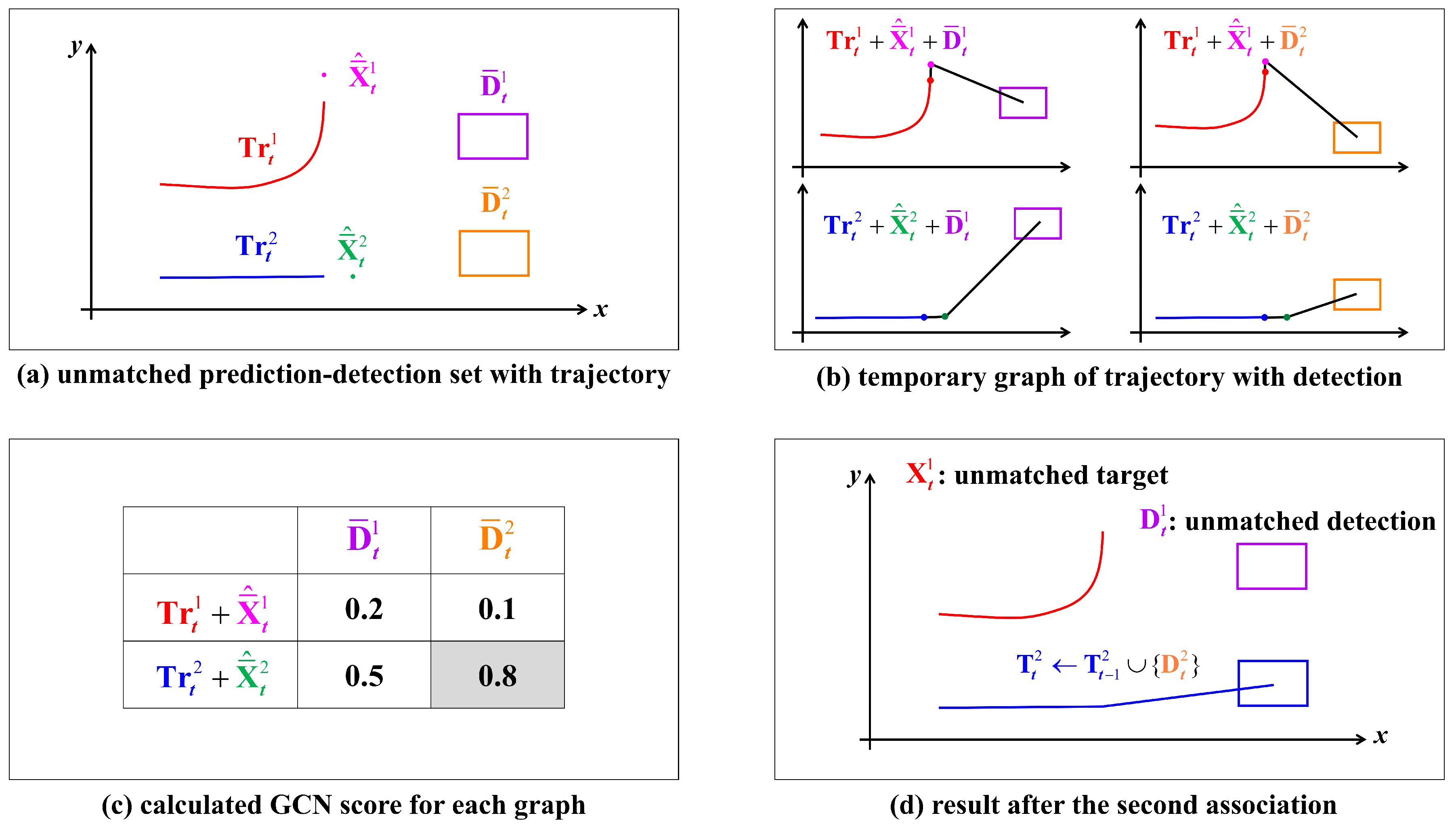
• A long-term association method using Graph Convolutional Networks (GCNs) to link the historical trajectories of targets with challenging detections is introduced.
• The proposed method relies solely on the current LiDAR frame data and past detection results, making it well-suited for real-time and online applications. By eliminating the requirement for supplementary data such as a map, the proposed approach becomes more practical and offers improved efficiency in real-world scenarios.
• An effective approach to manage unmatched targets is suggested, addressing issues related to short-term and long-term association. This strategy effectively manages occluded targets, ensuring more-reliable and -accurate tracking results.

The remainder of this paper is organized as follows. Section 2 briefly introduces the related works including TbD using a 3D LiDAR and graph-based tracking methods. Section 3 explains the proposed multi-level tracking method, which exploits the short-term and long-term relation between the detection and the existing tracks using the GCN. Section 4 shows the effectiveness of the experiment by applying it to the KITTI MOT dataset. Finally, some conclusions are drawn in Section 5.

2. Related Works

In this section, related works relevant to the proposed methods are introduced. Firstly, 3D-point-cloud-based deep learning applications for detection and robotics are introduced. Secondly, previous works on TbD using 3D LiDAR point clouds are presented. Thirdly, a review of graph-based MOT methods is provided.

2.1. Three-Dimensional-Point-Cloud-Based Deep Learning Applications for Detection and Robotics

In this section, relevant research on point cloud detection in the context of the TbD algorithm and studies related to 3D feature learning will be explored. Point cloud detection in 3D can be broadly categorized into two approaches: those employing machine learning and those leveraging deep learning techniques. In [17,18,19], object detection using machine learning methodologies was investigated. These methods often entail segmenting the LiDAR point cloud into objects, extracting features from each object, and subsequently, classifying object types using machine learning techniques. The advent of deep learning has significantly enhanced detection performance by training deep neural networks on these extracted features. Reference [20] combined a Region Proposal Network (RPN) and a PointNet-based object-detection network, delivering precise and efficient object detection in LiDAR data. Additionally, Reference [21] enhanced 3D object detection through a fusion of voxel and point methods, memory optimization, and the introduction of key point scene encoding and multi-scale RoI features. Reference [22] proposed an efficient 3D-object-detection method that enhances object representation, introduces an attention sparsity scheme, and employs hybrid positional embedding to integrate geometric–semantic information seamlessly. Reference [23] introduced the VirConv operator, which efficiently encodes the voxel features and extends the receptive field of 3D sparse convolution into the 2D image space. This extension effectively reduces the influence of noisy points, contributing to improved data processing and object recognition. In the field of robotics, another prominent application area for 3D point clouds, has the primary research focus on semantic segmentation mainly been conducted. It is essential for enabling robots to understand and interact with their environments effectively, as it serves as a foundational element for tasks such as object recognition and scene understanding. For instance, Reference [24] introduced a fast-moving object segmentation method using 3D LiDAR point clouds, incorporating residual images to achieve frame rates exceeding 10 Hz. Reference [25] presented an efficient framework for range-based object segmentation, which included range residual images, a highly effective meta-kernel feature extraction method, and a multi-scale feature aggregation module. Reference [26] proposed a mask-based panoptic segmentation approach that eliminates the need for dataset-specific hyperparameter tuning while maintaining competitive performance with a straightforward feature extractor.

2.2. Tracking-by-Detection in 3D LiDAR Point Clouds

Recent studies in object tracking predominantly employ Tracking-by-Detection methodologies. These approaches involve associating current detections with predictions derived from previous time frames. As one of the fields of object tracking, several research methods have been explored to enhance the performance by incorporating point cloud completion, with the goal of ensuring the stable tracking of partially detected objects [27,28,29]. Reference [27] suggested VPC-Net, an end-to-end network designed for completing 3D vehicle shapes from partial and sparse point clouds. This network comprises a unique encoder module for global feature extraction and a refiner module for preserving details and incorporates spatial transformer networks and point feature enhancement. Reference [28] proposed a motion-centric approach for real-time 3D LiDAR Single-Object Tracking (SOT). This approach does not rely on appearance matching, but instead, utilizes a second-stage pipeline called M2-Track. In the 1st stage, it predicts the target’s bounding box based on relative motion, and in the 2nd stage, it refines it using a denser point cloud from two partial target views and their relative motion. In [29], a Target Knowledge Transfer (TKT) module was introduced, which utilizes attention-based mechanisms to enhance the completion of template features. This enhancement is achieved by incorporating Adaptive Refine Prediction (ARP) techniques, specifically designed to address the issue of score–accuracy imbalance. In the domain of Multi-Object Tracking (MOT), many methods have been developed, each exploring various criteria for association and prediction. One such approach, detailed in [1], employs Kalman filters for object prediction, calculates the 3D Intersection over Union (IoU) between current detections and predictions, and utilizes the Hungarian algorithm for association. Conversely, the authors of [3] employed a similar Kalman-filter-based prediction method, but used the Mahalanobis distance as the association criterion, differing from [1]. Recently, research has been progressing to enhance MOT by cooperative interactions among multiple vehicles [30,31] due to the advancement of datasets related to cooperative vehicles [32,33]. Reference [30] presented a connected infrastructure that utilizes LiDAR roadside units, providing details on background filtering, object clustering, lane identification, and tracking. In [31], a framework was proposed that leverages historical object tracking data to enhance object detection, using a spatial–temporal deep neural network and a novel detection head to fuse detection and tracking features, particularly in scenarios with occlusion and out-of-range issues. In contrast, the work presented in [15] introduces a 3D MOT and motion forecasting approach that combines LiDAR data with high-definition maps, particularly in complex urban environments. A tracking method [11] that involves extracting the features of the 3D detection box and using the similarity between these features as an association cost has also been proposed. Further innovations aim at improving prediction accuracy in 3D LiDAR MOT, addressing the challenge posed by the limited point cloud data available for distant objects, compared to image-based methods. Proposed methods for more-accurate predictions include the cubature Kalman filter [34] and the precedence-guided association module for enhanced association [35]. Additionally, several MOT methods, such as [8,9,10,36], explore the fusion of LiDAR and camera detection results to compensate for the deficiencies of each sensor. However, these approaches are susceptible to inevitable detection failures or occlusions, as discussed in Section 1, where ID switching occurs when targets remain invisible for a specific number of frames.

2.3. Graph-Based MOT

To address the challenges associated with detection failures, another approach to MOT has emerged—the graph-based method. This method involves representing each target’s trajectory as a graph and employing it to facilitate associations between detections and tracks. While primarily explored in image-based MOT, this approach presents promising alternatives. For instance, Reference [37] proposed constructing a graph with detection boxes as vertices and associations between boxes as edges. This graph is then used for association through the binary classification of each edge, facilitated by a neural message-passing network, which extracts the features from each box. In [38], two types of graphs, an appearance graph network and a motion graph network, were introduced for MOT. These graphs calculate the similarity between detected objects and tracker predictions and combine these values through a weighted summation for the association. The authors in [39] presented MOT methods based on Graph Neural Networks (GNNs) with 2D and 3D feature learning. Appearance and motion features are extracted from each sensor, and a graph is constructed from the fused features. The graph’s nodes are updated through feature aggregation, and the affinity matrix is computed with the edge regression module. Furthermore, Reference [40] introduced an association approach focused on infra-frame relationships, represented as a general undirected graph. This work proposes a general graph-matching algorithm to solve the association problem by expressing relationships between tracklets and infra-frame detections. Despite successful 2D MOT methods in the image domain, challenges remain in representing dynamics and associations in the 3D LiDAR domain, leading to estimation deficiencies. However, the proposed method takes a trajectory-based approach, creating actual object motion trajectories and performing association based on this novel perspective. Meanwhile, several tracklet-based MOT methods designed for 3D LiDAR have also emerged. In [14], a unified framework was introduced that integrates detection, tracking, and motion forecasting into a single-stage process, leveraging 3D LiDAR data. This approach utilizes multiple consecutive temporal frames as the input, enabling the accurate extraction of 3D bounding boxes, which encompass both spatial and temporal dimensions. In [13], a MOT approach focused on tracklet association using a tracklet proposal network, involving sequence-based point clouds as the inputs. The method generates tracklet candidates by performing object proposal generation and motion regression on spatial–temporal point cloud features. It then refines these proposals and generates the final tracking results by associating refined tracklets with previous trajectories. However, these approaches necessitate both current and past LiDAR data, making them less suitable for real-time or online applications. In contrast, the proposed method was designed for real-time deployment, requiring only the current LiDAR frame for association with past track information.

3. Proposed Method

Figure 3 shows the architecture of the proposed multi-level MOT algorithm using a 3D LiDAR. It takes the TbD approach: It detects some objects each time and, then, associates them with the predictions from the existing tracks using various criteria. The objective of 3D MOT is to find the optimal association between 3D detections and the existing tracks so that consistent identification for each tracked object can be maintained even when the objects are occluded or interact with other objects. In the following subsections, the components of the proposed approach will be explained in detail.

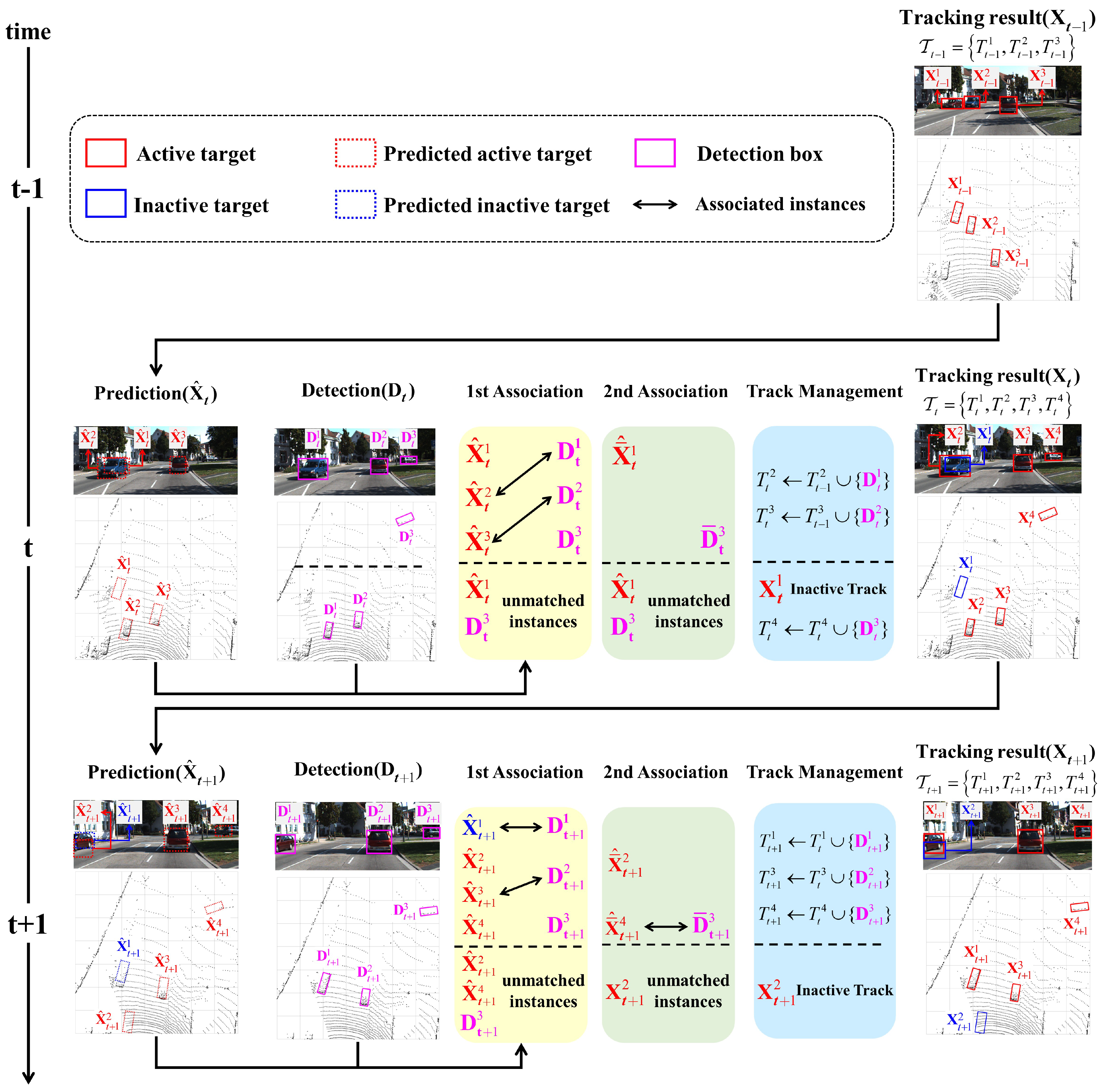
3.1. State Definition

Since the TbD approach is employed in the proposed MOT method, it is assumed that the output from the 3D detector at time t is given by

$$\begin{array}{c}\hfill {\mathbf{D}}_t^i=(x_t^i,y_t^i,z_t^i,w_t^i,h_t^i,l_t^i,{\theta }_t^i)(i=1,\cdots ,M_t)\end{array}$$

(1)

where $M_t$ is the number of the detection boxes at time t; $(x_t^i,y_t^i,z_t^i),(w_t^i,h_t^i,l_t^i)$, and ${\theta }_t^i$ denote the position, the size, and the orientation of the detection boxes, respectively. Many off-the-shelf 3D detectors such as [20,21,22,23] can be used as the detector, and the one of [20] was used in this paper. Further, it is supposed that a set of tracks $T_{t-1}=\left\{{\mathbf{T}}_{t-1}^j\right|j=1,\cdots ,N_{t-1}\}$ is given at time t − 1, where $N_{t-1}$ is the number of tracks maintained at time t − 1, and the jth track ${\mathbf{T}}_{t-1}^j$, which was initialized $t_j$ time steps ago, is given by

$$\begin{array}{c}\hfill {\mathbf{T}}_{t-1}^j=\left\{{\mathbf{X}}_{t-t_j}^j,{\mathbf{X}}_{t-(t_j-1)}^j,\cdots ,{\mathbf{X}}_{t-2}^j,{\mathbf{X}}_{t-1}^j\right\}\end{array}$$

(2)

where

$$\begin{array}{c}\hfill {\mathbf{X}}_{t-1}^j=(x_{t-1}^j,y_{t-1}^j,z_{t-1}^j,w_{t-1}^j,h_{t-1}^j,l_{t-1}^j,{\theta }_{t-1}^j,v_{t-1}^j,{\dot{\theta }}_{t-1}^j,{\dot{z}}_{t-1}^j)\end{array}$$

(3)

Here, ${\mathbf{X}}_{t-1}^j$ is the latest state of the jth track ${\mathbf{T}}_{t-1}^j$. If ${\mathbf{D}}_t^i$ and ${\mathbf{X}}_{t-1}^j$ are compared, it can be seen that they have similar information, except $v_{t-1}^j$, ${\dot{\theta }}_{t-1}^j$ and ${\dot{z}}_{t-1}^j$, where $v_{t-1}^j$ is the velocity of the jth track ${\mathbf{X}}_{t-1}^j$ at time t − 1. All the variables are depicted in Figure 3.

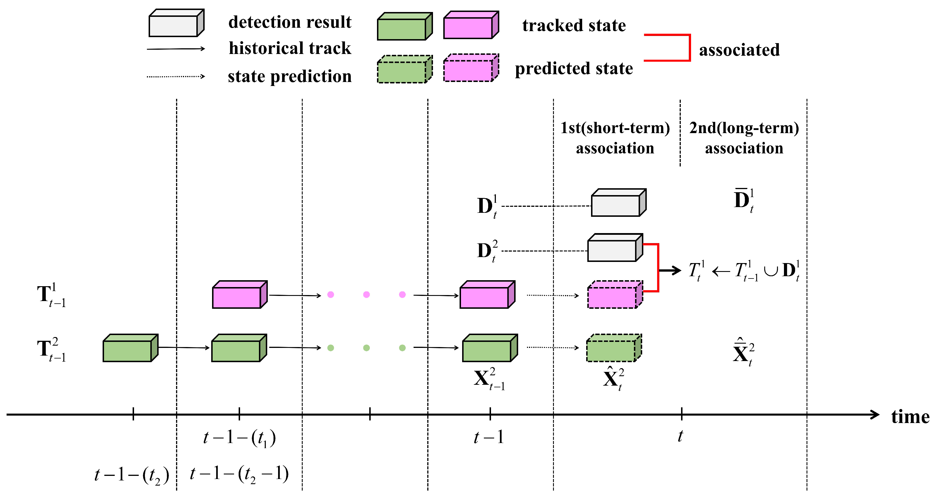
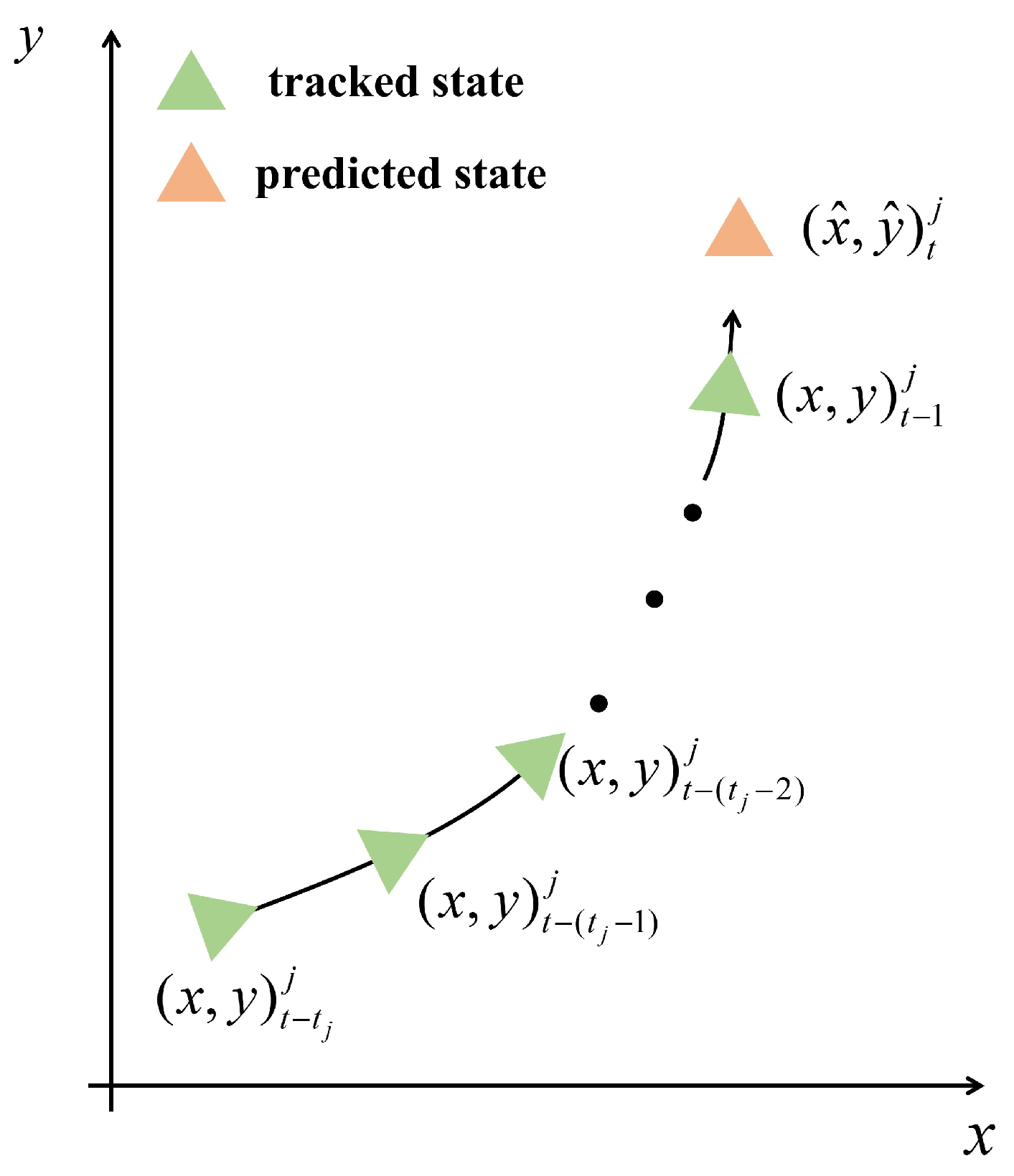
3.2. State Prediction

In this step, the evolution of the latest states of the maintained tracks $T_{t-1}=\left\{{\mathbf{T}}_t^j\right|j=1,\cdots ,N_{t-1}\}$ at time t − 1 is predicted by the Constant Turn Rate and Velocity (CTRV) motion model in [41]. Specifically, when the latest state ${\mathbf{X}}_{t-1}^j$ is given from the jth track ${\mathbf{T}}_{t-1}^j=\left\{{\mathbf{X}}_{t_j}^j,{\mathbf{X}}_{t_j+1}^j,\cdots ,{\mathbf{X}}_{t-2}^j,{\mathbf{X}}_{t-1}^j\right\},$ the corresponding future state ${\widehat{\mathbf{X}}}_t^j$ at time t is represented by

$${\widehat{\mathbf{X}}}_t^j={\mathbf{X}}_t^j+{\left[\begin{array}{c}\frac{v}{\dot{\theta }}\left(\mathit{sin}\left(\theta +\dot{\theta }\Delta t\right)-\mathit{sin}\theta \right)\\ \frac{v}{\dot{\theta }}\left(-\mathit{cos}\left(\theta +\dot{\theta }\Delta t\right)+\mathit{cos}\theta \right)\\ \dot{z}\Delta t\\ 0\\ 0\\ 0\\ \dot{\theta }\Delta t\\ 0\\ 0\\ 0\end{array}\right]}^{\mathit{T}}$$

(4)

where $t_j$ denotes the length of the jth track and $\Delta t$ is the sampling time. In contrast to prior 3D MOT studies, which employed either Constant Velocity (CV) modeling techniques [1,3], RNN models [42,43], or LSTM models [44,45], the CTRV model was used to decrease the computational burden and predict more-realistic and smoother trajectories. Moreover, the CTRV model is particularly well suited for scenarios with complex motion patterns, as it can effectively handle the nonlinearities associated with turning. This enables the accurate representation and prediction of trajectories involving curved paths or direction changes within complex environments.

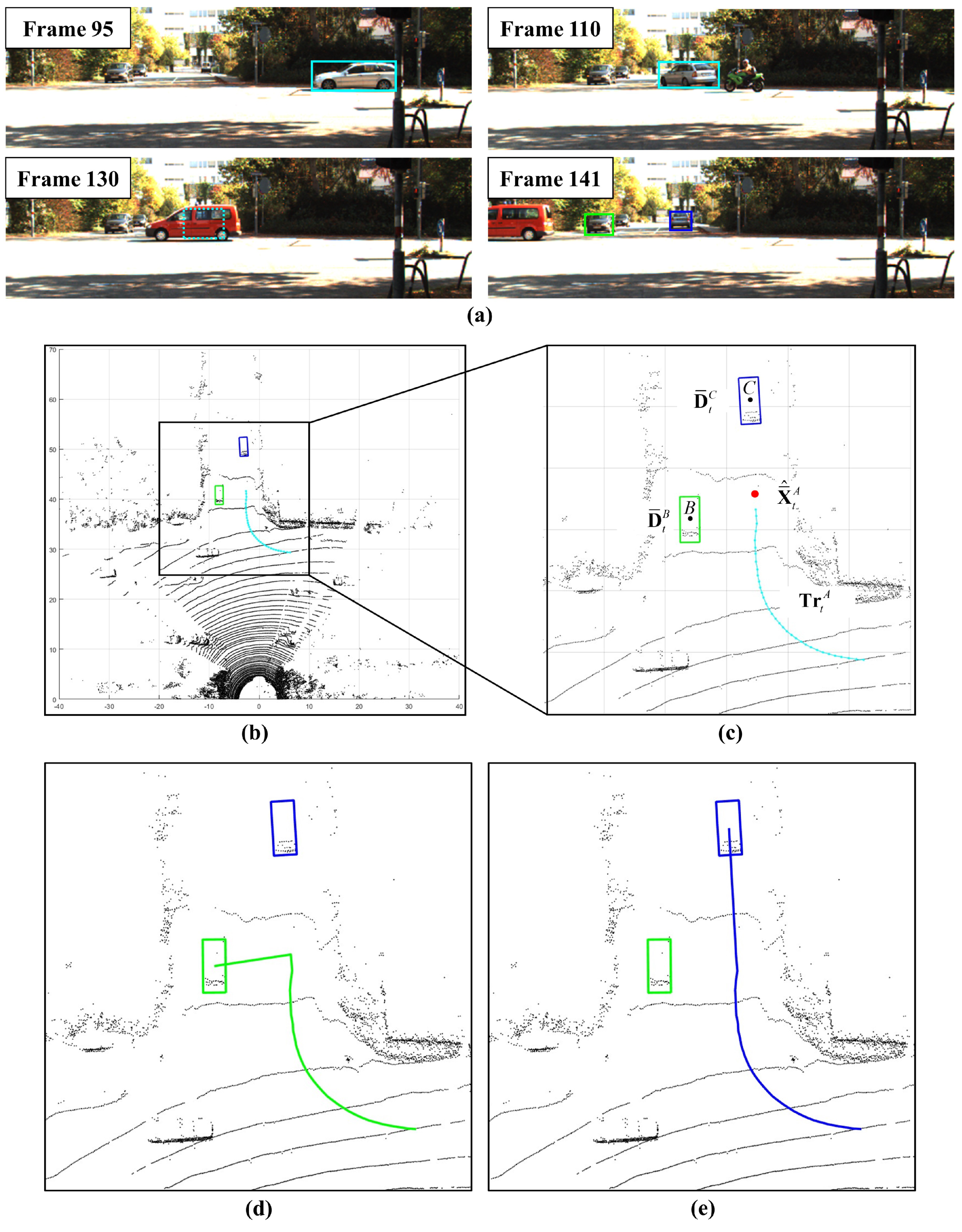
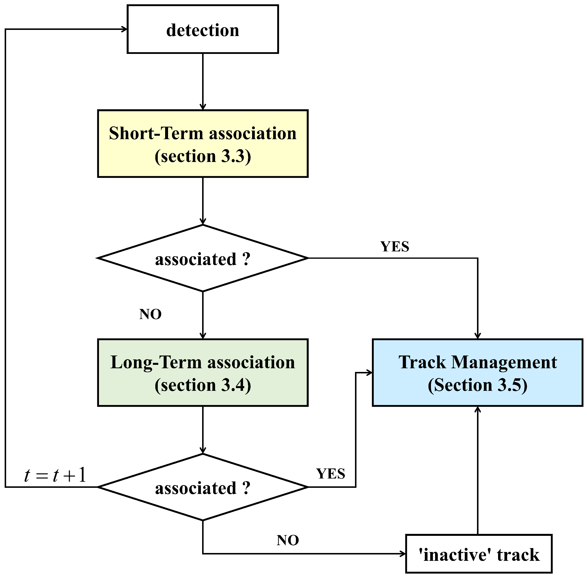
3.3. First Association Based on Short-Term Relation

In this step, the first association between the predicted state ${\widehat{\mathbf{X}}}_t$ and the detection ${\mathbf{D}}_t$ in the 3D LiDAR domain was conducted to maximize the matching weight between the two sets by the Hungarian algorithm [46]. Here, the matching cost $\mathbf{C}(i,j)$ between the two sets ${\mathbf{D}}_t^i$ and ${\widehat{\mathbf{X}}}_t^j$ is defined in [1] by

$$\begin{array}{c}\hfill \mathbf{C}(i,j)=\frac{{\mathbf{I}}_V}{{\mathbf{U}}_V}=\frac{{\mathbf{I}}_V}{{\mathbf{V}}_{D_t}+{\mathbf{V}}_{{\widehat{X}}_t}-{\mathbf{I}}_V}\end{array}$$

(5)

where ${\mathbf{V}}_{D_t}$ and ${\mathbf{V}}_{{\widehat{X}}_t}$ are the volumes of ${\mathbf{D}}_t^i$ and ${\widehat{\mathbf{X}}}_t^j$, respectively; ${\mathbf{I}}_V$ and ${\mathbf{U}}_V$ are those of the intersection and the union between ${\mathbf{D}}_t^i$ and ${\widehat{\mathbf{X}}}_t^j$, respectively. More specifically, to calculate ${\mathbf{I}}_V$ and ${\mathbf{U}}_V$, ${\mathbf{D}}_t^i$ and ${\widehat{\mathbf{X}}}_t^j$ are projected onto a two-dimensional representation from a bird’s-eye view. Subsequently, the projected area is multiplied by the corresponding height to obtain the results. The definition of the matching cost given in Equation (5) is based on the observation that vehicles cannot suddenly accelerate or turn sharply beyond a certain level. An affinity matrix of size $M_t\times N_t$ is constructed using the matching cost provided by Equation (5). The bipartite association is then made between ${\mathbf{D}}_t^i$ and ${\widehat{\mathbf{X}}}_t^j$, with $M_t$ representing the number of current detections and $N_t$ denoting the number of existing tracks at time t. After the first association based on the short-term relation, the sets of new detections and the predictions from the existing tracks are divided into the matched pairs (=track update) and unmatched instances. For example, it was assumed that three tracks $T_{t-1}=\{T_{t-1}^1,T_{t-1}^2,T_{t-1}^3\}$ exist at time t − 1, the scenario in Figure 3. The latest states ${\mathbf{X}}_{t-1}^1$, ${\mathbf{X}}_{t-1}^2$, and ${\mathbf{X}}_{t-1}^3$ of the existing tracks $T_{t-1}$ are updated (predicted) as ${\widehat{\mathbf{X}}}_t^1$, ${\widehat{\mathbf{X}}}_t^2$, and ${\widehat{\mathbf{X}}}_t^3$, respectively. Then, it was supposed that three detections $D_t=\{{\mathbf{D}}_t^1,{\mathbf{D}}_t^2,{\mathbf{D}}_t^3\}$ are given at time t. If ${\widehat{\mathbf{X}}}_t^2$ and ${\widehat{\mathbf{X}}}_t^3$ are associated with ${\mathbf{D}}_t^1$ and ${\mathbf{D}}_t^2$, respectively, the corresponding tracks $T_{t-1}^2$ and $T_{t-1}^3$ will be updated by $T_t^2\stackrel{}{\leftarrow }{T}_{t-1}^2\cup \left\{{\mathbf{D}}_t^1\right\}$ and $T_t^3\stackrel{}{\leftarrow }{T}_{t-1}^3\cup \left\{{\mathbf{D}}_t^2\right\}$, respectively. In this case, the Kalman filter or other filters can be applied to update ${\widehat{\mathbf{X}}}_t^2$ and ${\widehat{\mathbf{X}}}_t^3$, but they were not utilized as they did not make much of a difference. The track $T_{t-1}^1=\left\{{\mathbf{X}}_{t-1}^1\right\}$ and the measurement ${\mathbf{D}}_t^3$ remained as the unmatched instances, as shown in Figure 3.

3.4. Second Association Based on Long-Term Relation

The first association based on the short relationship might not be enough when a tracked object becomes temporarily hidden or obscured from view, making it challenging to maintain a continuous association. Figure 4a depicts an example where the first association failed. As seen in Figure 4a, a vehicle turning at an intersection is occluded at Frame 124 and is detected again six frames later at Frame 130. Figure 4b shows the trajectories before and after the occlusion in the situation of Figure 4a. The trajectory colored in red corresponds to the motion of the vehicle before the occlusion, indicating its path up until the point of disappearance (=occlusion). On the other hand, the trajectory colored in blue corresponds to the motion of the vehicle after the vehicle re-appears from Frame 130 and comes back into view. Occlusion occurred during the space between the red and blue trajectories. When relying solely on the first short-term association, the object that re-appears at Frame 130 cannot be assigned the same ID that the vehicle had before the occlusion at Frame 124 because the predicted target and the detection do not overlap, making the IoU zero. In such situations, ID switching occurs, which is indicated by the change of the trajectory color from red to blue.

To solve the problem, a long-term association that exploits the historical trajectory of the existing track is proposed. This approach aims to mitigate ID switching and improve the overall performance of the tracking system. Even when the trajectory of the same object is divided into two segments, if the two segments exhibit similar-looking behavior, the connection of the two segments is made, creating a path even after occlusion. By leveraging this idea, the association method relies on long-term relationships to handle situations where a prediction–detection pair remains unmatched after the 1st association is proposed. The proposed method considers objects’ historical information and trajectory patterns to establish the associations beyond the immediate frame, ensuring a more-robust and -accurate tracking process. Thus, when the previously disappeared target reappears, it would be possible to maintain the existing ID rather than assign a new one. By considering the long-term relationship between tracks and detections, the proposed method aims to improve the overall tracking performance and handle cases where immediate associations are not feasible. For example, as shown in Figure 5, it was supposed that ${\mathbf{D}}_t^1$ and ${\widehat{\mathbf{X}}}_t^2$ remain unmatched after the first association, and these two are employed as the inputs of the second association. In this situation, ${\mathbf{D}}_t^1$ and ${\widehat{\mathbf{X}}}_t^2$ will be re-named as ${\overline{\mathbf{D}}}_t^1$ and ${\widehat{\overline{\mathbf{X}}}}_t^2$, respectively, where the “bar” means the instances that remain unmatched after the first association.

Moreover, for the second association, the trajectory ${\mathbf{Tr}}_t^j$ is also defined as ${\mathbf{Tr}}_t^j{=\{(x,y)}_{t-t_j}^j$, ${(x,y)}_{t-(t_j-1)}^j,\cdots ,{(x,y)}_{t-1}^j\}$, generated by connecting the coordinates from the entire track ${\mathbf{T}}_t^j$, where it was initialized $t_j$ time steps ago. The latest time of the trajectory ${\mathbf{Tr}}_t^j$ is denoted as t − 1 since this target is not associated with it at time t, but is associated until time t − 1. An example figure explaining ${\mathbf{Tr}}_t^j$ is shown in Figure 6.

An example of the proposed GCN-based long-term association procedure is depicted in Figure 7, and the steps are as follows: The inputs of the 2nd association consist of the unmatched track and the detection set after the 1st association. In Figure 7a, the scenario assumes that, after the 1st association, two targets have not been matched with any detections, and there are also two detections that have not been matched with any targets. To generate trajectory candidates, all possible combinations of tracks (${\overline{\mathbf{D}}}_t^i$, ${\widehat{\overline{\mathbf{X}}}}_t^j$, and ${\mathbf{Tr}}_t^j$) are connected with the detection set. In this case, as depicted in Figure 7b, a total of four trajectory candidates are generated by considering all target–detection sets. If ${\overline{\mathbf{D}}}_t^i$ and ${\widehat{\overline{\mathbf{X}}}}_t^j$ are the same object, the trajectory connecting the two points, along with ${\mathbf{Tr}}_t^j$, as illustrated in Figure 4b, will exhibit the same directivity, and this indicates a high classification score in the GCN. Hence, as depicted in Figure 7c, the GCN score is calculated for each trajectory candidate. The graph for the GCN is constructed as follows: The nodes of the graph are composed of the coordinates of ${\overline{\mathbf{D}}}_t^i$, ${\widehat{\overline{\mathbf{X}}}}_t^j$, and ${\mathbf{Tr}}_t^j$. The input graph for the GCN is connected ${(x,y)}_{t-1}^j$, the most-recent coordinates of ${\mathbf{Tr}}_t^j$, with ${\widehat{\overline{\mathbf{X}}}}_t^j$ and, then, further connects with ${\overline{\mathbf{D}}}_t^i$, maintaining the chronological order of these three components. The classification score of the GCN’s output is then used to determine the validity of the generated paths. To clarify, the GCN score reflects the likelihood that two instances denoted as ${\overline{\mathbf{D}}}_t^i$ and ${\widehat{\overline{\mathbf{X}}}}_t^j$ represent the same object. A high GCN score indicates a strong connection between the trajectory of these instances. Consequently, associations between the tracking–detection sets of the generated candidates are established when their scores surpass a predetermined threshold. Referring to the table in Figure 7c, it is evident that the validity scores of all detections associated with ${\widehat{\overline{\mathbf{X}}}}_t^1$ fell below the threshold. As a result, ${\widehat{\overline{\mathbf{X}}}}_t^1$ remained unmatched even after the second association.

On the other hand, consider ${\widehat{\overline{\mathbf{X}}}}_t^2$, which exhibits an exceeding GCN score with ${\overline{\mathbf{D}}}_t^2$. In this case, the corresponding track ${\widehat{\overline{\mathbf{X}}}}_t^2$ will be updated as follows: $T_t^2\stackrel{}{\leftarrow }{T}_{t-1}^2\cup \left\{{\mathbf{D}}_t^2\right\}$. This update occurs due to the high GCN score for the trajectory connecting ${\widehat{\overline{\mathbf{X}}}}_t^2$ and ${\overline{\mathbf{D}}}_t^2$, surpassing the threshold. Simultaneously, ${\overline{\mathbf{D}}}_t^1$ becomes an unmatched detection, resulting in the scenario illustrated in Figure 7d. This outcome demonstrates the dynamic nature of the proposed tracking and association methodology, where GCN-based scoring plays a crucial role in determining valid object trajectories.

Figure 8 provides a real data example of tracking using the proposed second association based on the long-term association. In Figure 8a, the situation before and after an occlusion is illustrated. In Frames 95 and 110 (top-left and top-right), a cyan-colored vehicle is seen making a right turn at an intersection, with the front view of the ego-vehicle assumed to be facing north. This vehicle was tracked for approximately 35 frames, but becomes occluded by another vehicle moving straight from east to west of the intersection at Frame 130. Due to this occlusion, the tracked vehicle is not detected for 10 frames. However, in Frame 141, it is detected again and marked as blue (note that it is shown in a color other than cyan to depict the progress of the proposed method). Figure 8b shows the LiDAR domain view of the situation at Frame 141, and Figure 8c provides an enlarged view of specific areas within Figure 8b. In Figure 8c, it is observed that the red point labeled as A represents the predicted position of the existing track (marked as cyan). However, Point A cannot be associated with either the green or blue box in the image. In this scenario, the proposed second association method is applied.

In Figure 8c, Points B and C represent the center points of the unmatched detection boxes after the first association (referred to as ${\overline{\mathbf{D}}}_t^B$ and ${\overline{\mathbf{D}}}_t^C$). Point A represents the predicted location of the unmatched track, ${\widehat{\overline{\mathbf{X}}}}_t^A$, and the cyan trajectory indicates the trajectory from the time of the initial track initialization to before the occlusion, ${\mathbf{Tr}}_t^A$. Figure 8d,e showcase the temporary trajectories created by connecting point ${\overline{\mathbf{D}}}_t^B$(or ${\overline{\mathbf{D}}}_t^C$) with points ${\widehat{\overline{\mathbf{X}}}}_t^A$ and ${\mathbf{Tr}}_t^A$, respectively. Upon examining Figure 8d,e, it becomes apparent that the GCN score for a point ${\overline{\mathbf{D}}}_t^C$ is higher than that of point ${\overline{\mathbf{D}}}_t^B$, and this score surpasses the threshold. Consequently, it can be inferred that the object with Center Point C is the same as the initially initialized object in Frame 95, employing the proposed second association. Previous MOT methods [1,2,3] typically initialize it as a new target if it remains unassociated for a certain number of frames after the occlusion. This can lead to ID switching errors, where the object detected in Frame 141 would be considered a new target. In contrast, by utilizing the proposed second association, it becomes possible to identify the object that was occluded for a long period (10 frames in this example) as the same object, resulting in more-stable tracking.

3.5. Track Management

While the proposed approach incorporates two-level associations in Section 3.3 and Section 3.4, there can still be unmatched tracks or detections. Existing MOT methods [1,2,3] typically handle unmatched tracks by employing a threshold age mechanism, wherein a track is deleted and re-initialized if it remains unmatched for a specific duration. This threshold age is a critical parameter, and finding the optimal value requires careful consideration. Using smaller threshold age values may lead to reduced tracking performance, as temporarily missed objects may not be effectively tracked and removed. Conversely, larger threshold age values can decrease tracking accuracy due to the possibility of erroneous associations caused by unmatched targets lingering within the sensor’s Field of View (FoV), leading to increased data association mismatches.

In this paper, a solution to address these challenges is proposed by introducing an “inactive” state for targets that cannot be matched even after employing the short-term and long-term association techniques. These “inactive” tracks undergo the same prediction method as other tracks and remain in this state until a successful association is established. If the predicted “inactive” target cannot be associated with any detections in the frame following its exit from the sensor’s Field of View (FoV), that track is eliminated in the subsequent frame. This approach significantly improves tracking performance compared to existing methods. Additionally, any unmatched detections are initialized as new tracks, and their associated targets are updated using the detection results.

4. Experiment

In this section, a real-world dataset for autonomous driving applications is employed to validate the performance of the proposed method. Through comparative experiments, the proposed method outperformed several other well-known tracking methods, 3D LiDAR-based methods, as well as camera–LiDAR sensor fusion methods.

4.1. Dataset and Experiment Settings

The KITTI benchmark tracking dataset [47] was utilized as the evaluation platform. This dataset provides 21 training sequences and 29 test sequences of front-view camera images and 3D LiDAR point clouds. The training and test sequences contain a total of 8008 and 11,095 frames, respectively. The 3D LiDAR point clouds in the KITTI dataset were produced by recording with a Velodyne HDL-64E LiDAR, manufactured by Velodyne Lidar, Inc. in California, USA. In the experiments, the 2D camera data were not used for the proposed algorithm, but for visualization to see the results more clearly. The proposed method was implemented on a personal computer equipped with an Intel Core i7-6700 CPU, 64 GB of RAM, and an NVIDIA TITAN Xp GPU. The proposed MOT method averaged about 40 ms (25 FPS) per LiDAR frame on the KITTI dataset, using the previously mentioned computer environment.

4.2. Evaluation Metrics

The quantitative performance verification of the proposed method was performed by projecting the 3D tracking result into the 2D image plane. After that, the CLEAR MOT metric [48], which is the most-used for the KITTI tracking benchmark, was employed to evaluate the tracking performance. Brief descriptions of the metrics used in the evaluation are as follows. The Multi-Object Tracking Accuracy (MOTA), which calculates the overall tracking performance, is defined as

$$\begin{array}{c}\hfill MOTA=1-\frac{{\sum }_t{m}_t+f{p}_t+mm{e}_t}{{\sum }_{t}G{T}_t}\end{array}$$

(6)

where $m_t$, $f{p}_t$, $mm{e}_t$, and $G{T}_t$ are the number of misdetections, false positives, mismatches, and the ground truth for the entire time t, respectively. The Multi-Object Tracking Precision (MOTP) metric was used to measure the object localization precision, which is defined as:

$$\begin{array}{c}\hfill MOTP=\frac{{\sum }_{t,i}{d}_t^i}{{\sum }_t{c}_t}\end{array}$$

(7)

where $d_t^i$ is the overlap between the ith prediction box and the corresponding ground truth box and $c_t$ represents the total number of matches between the detection and ground truth for the entire time t. Fragmentation (FRAG) calculates the number of frames in which a complete whole path splits, i.e.,it measures the times disturbed during tracking, and ID Switching (IDS) is counted by the number of mismatches in the entirety of the tracking. Recently, Higher-Order Tracking Accuracy (HOTA) [49] has been suggested as another MOT evaluation metric, which is different from CLEAR metrics, and it is mainly employed in the KITTI dataset as one of the main evaluation metrics for tracking performance. HOTA considers the equilibrium of accurate detection, correct association, and precise localization, and it can be decomposed into two sub-metrics, which are the Detection Accuracy (DetA) and Association Accuracy (AssA). Each of these is defined as follows:

$$\begin{array}{c}\hfill DetA=\frac{\left|TP\right|}{\left|TP\right|+\left|FN\right|+\left|FP\right|}\end{array}$$

(8)

$$\begin{array}{c}\hfill AssA=\frac{1}{\left|TP\right|}\sum _{i\in \left\{TP\right\}}\frac{\left|TPA\right(i\left)\right|}{\left|TPA\right(i\left)\right|+\left|FNA\right(i\left)\right|+\left|FPA\right(i\left)\right|}\end{array}$$

(9)

$$\begin{array}{c}\hfill HOTA=\sqrt{DetA\times AssA}\end{array}$$

(10)

In Equations (8) and (9), $\left|TP\right|$, $\left|FN\right|$, and $\left|FP\right|$ are the overall number of true positives, false negatives, and false positives in the total data, respectively. In Equation (9), $\left|TPA\right(i\left)\right|$, $\left|FNA\right(i\left)\right|$, and $\left|FPA\right(i\left)\right|$ represent the number of True Positive Associations (TPAs), False Positive Associations (FPAs), and False Negative Associations (FNAs), respectively. Each of these is explained as follows: The TPAs represent the number of correct associations made by the tracking system. In other words, it is the count of correctly identified tracked objects that match the ground truth annotations. The FPAs indicate the number of incorrect associations made by the tracking system. This refers to the situations where the tracking system identifies an object that does not have a corresponding ground truth annotation. The FNAs represent the number of missed associations by the tracking system. It refers to the situations where the tracking system fails to identify an object that should have been tracked according to the ground truth annotations. In this paper, both the CLEAR and HOTA metrics were selected for MOT performance evaluation.

4.3. Quantitative Result

Many papers regarding 3D Tracking-by-Detection (TbD) MOT have used PointRCNN [20] as a 3D detector. Thus, PointRCNN [20] was also used as a detector for a fair comparison with the previous methods. In

Table 1. Quantitative results compared to other 3D LiDAR-based MOT methods on the test set of the KITTI dataset. In the first row of the table, “↑” indicates the higher the value, the better the performance, and ”↓” means vice versa. Methods with mark “#” use PointRCNN [20] as the 3D detector. The values showing the best performance for each metric are indicated in bold. The results are obtained from https://www.cvlibs.net/datasets/kitti/eval_tracking.php (accessed on 5 October 2023).

Method (Abbreviation)	HOTA (↑)	MOTA (↑)	MOTP (↑)	AssA (↑)	IDS (↓)	FRAG (↓)
Point3DT [50]	57.20%	67.56%	76.83%	59.15%	294	756
AB3DMOT [1] #	69.99%	83.61%	85.23%	69.33%	113	206
DiTNet [51]	72.21%	84.53%	84.36%	74.04%	101	210
PolarMOT [12] #	75.16%	85.08%	85.63%	76.95%	462	599
CenterTube [4]	71.25%	86.97%	85.19%	69.24%	191	344
Proposed method #	75.65%	85.03%	84.93%	80.02%	39	367

, the quantitative results of the proposed method are presented in comparison to the other 3D LiDAR-based MOT methods specifically for the “Car” category using the KITTI tracking test set. The results indicated that the proposed method outperformed the others in terms of the HOTA and AssA while exhibiting the lowest IDS.

The results presented in [12], which demonstrate a HOTA performance similar to the proposed method, and in [4], which exhibit a slightly higher MOTA performance compared to the proposed approach, were closely examined. Initially, the results of the proposed method and the method in [12] using the same detector were analyzed. While the MOTA performance was nearly identical, the method in [12] boasted an approximately 0.9% higher MOTP score. In contrast, the proposed method excelled in the AssA category, outperforming the method in [12] by approximately 3%. The AssA, as defined by Equation (9), signifies the degree to which the targets tracked by the proposed algorithm maintain their unique IDs. A high AssA score indicated that the proposed method demonstrated significantly lower IDS and FRAG than the method in [12]. In essence, this suggested that the proposed method provided more-robust tracking for individual objects with consistent IDs when using the same detector as the method in [12]. Now, the results of method [4] will be compared. The method in [4] demonstrated commendable performance on traditional tracking metrics, boasting a 2% higher MOTA and a 1% higher MOTP compared to the proposed method, showcasing its proficiency in basic object tracking and localization. However, the proposed method appeared to be a superior tracker, outperforming that in [4] with a 4% higher HOTA score, 11% higher AssA score, and significantly lower IDS. These results indicated that the proposed method is critical for complex tracking scenarios; therefore, based on the comprehensive evaluation of these performance metrics, the proposed method stood out as the preferred choice for robust and accurate object tracking.

Table 2. Quantitative result compared to other LiDAR–camera sensor fusion MOT methods on the test set of the KITTI dataset. In the first row of the table, “↑” indicates the higher the value, the better the performance, and ”↓” means vice versa. Methods with mark “#” use PointRCNN [20] as the 3D detector. The values showing the best performance for each metric are indicated in bold. The results are obtained from https://www.cvlibs.net/datasets/kitti/eval_tracking.php (accessed on 5 October 2023).

Method (Abbreviated)	HOTA (↑)	MOTA (↑)	MOTP (↑)	AssA (↑)	IDS (↓)	FRAG (↓)
MOTSFusion [52] #	68.74%	84.24%	85.03%	66.16%	415	569
JRMOT [36]	69.61%	85.10%	85.28%	66.89%	271	273
JMODT [9]	70.73%	85.35%	85.37%	68.76%	350	693
EagerMOT [8] #	74.39%	87.82%	85.69%	74.16%	239	390
Opm-NC2 [53] #	73.19%	84.21%	85.86%	73.77%	195	301
DeepFusionMOT [10] #	75.46%	84.63%	85.02%	80.05%	84	472
BcMOT [54]	71.00%	85.48%	85.31%	69.14%	381	732
StrongFusion-MOT [55]	75.65%	85.53%	85.07%	79.84%	58	416
Proposed method #	75.65%	85.03%	84.93%	80.02%	39	367

presents the quantitative results comparing the proposed method to other LiDAR–camera sensor fusion tracking methods, specifically for the “Car” category, using the KITTI tracking test set. As seen in Table 1, the proposed approach excelled in several critical tracking aspects, relying solely on 3D LiDAR data. The proposed method achieved the best performance according to the HOTA metric and recorded the lowest number of Identity Switches (IDSs).

Upon closer examination of Table 2, it is clear that the proposed tracking method maintained a commendable level of performance in dynamic scenarios. Notably, it matched the tracking accuracy of that in [55], a system that employs LiDAR–camera fusion, in terms of the Highest Overlap and Track Accuracy (HOTA) metric. Furthermore, the proposed method outperformed that in [55] in other vital aspects, including the Association Accuracy (AssA), Identity Switches (IDSs), and Fragmentation (FRAG) metrics. The higher AssA values reflected the proposed method’s proficiency in maintaining consistent object associations over time, while the lower IDS and FRAG values underscored its ability to minimize tracking inconsistencies and fragmented tracks. In summary, the proposed method offered robust tracking capabilities in dynamic scenarios, relying solely on 3D LiDAR data. These findings demonstrated the effectiveness of the proposed tracking strategy in providing robust performance in dynamic environments.

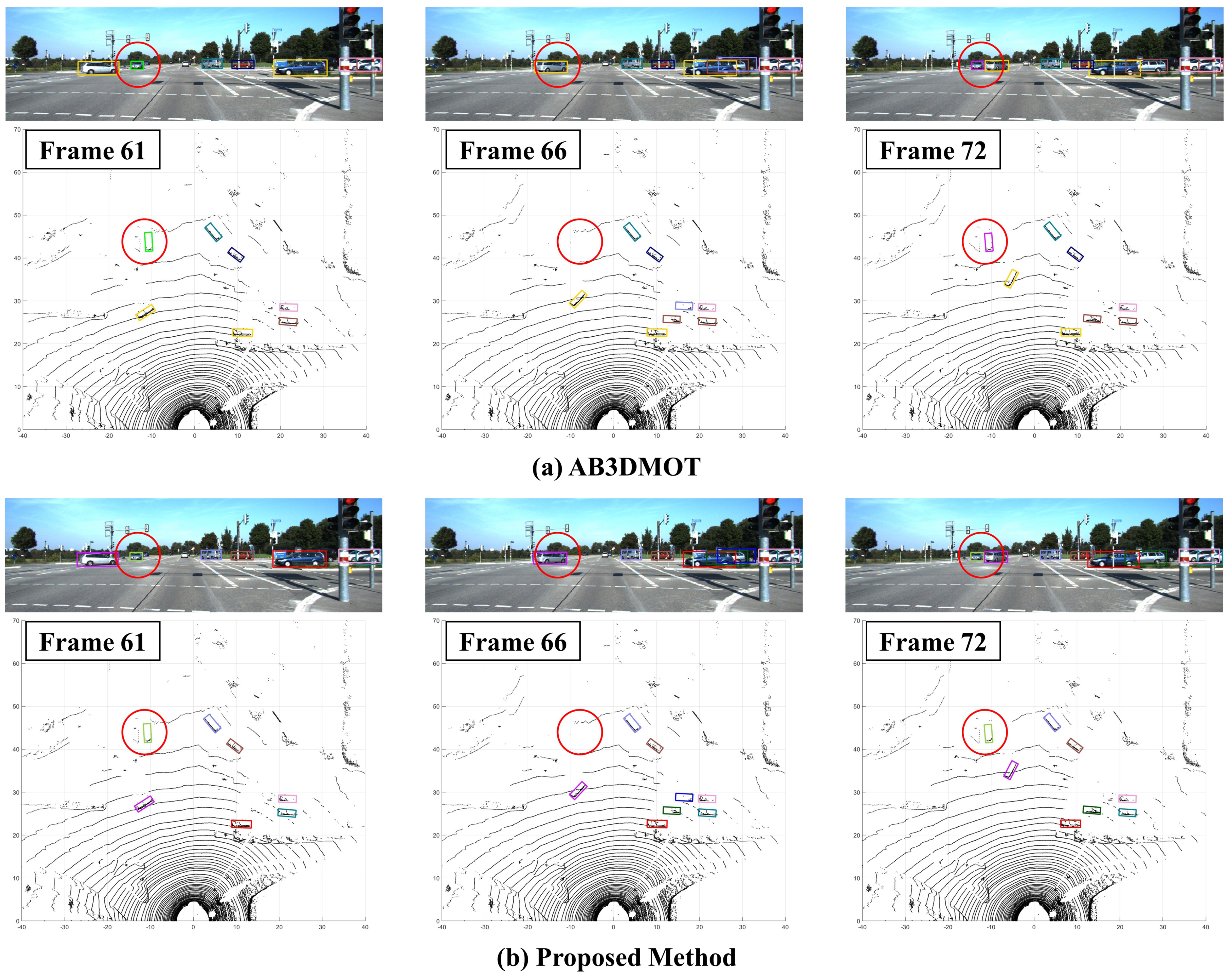
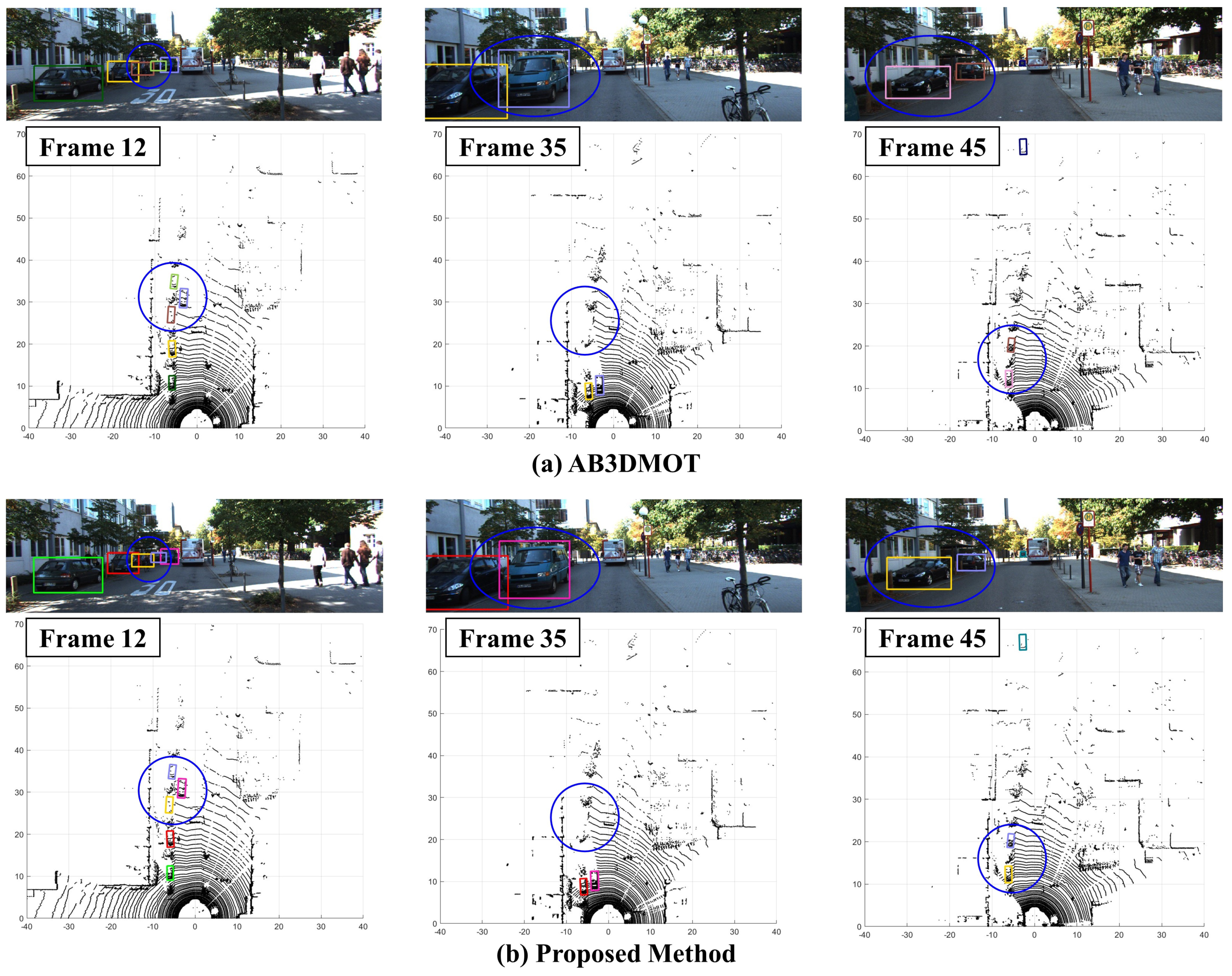
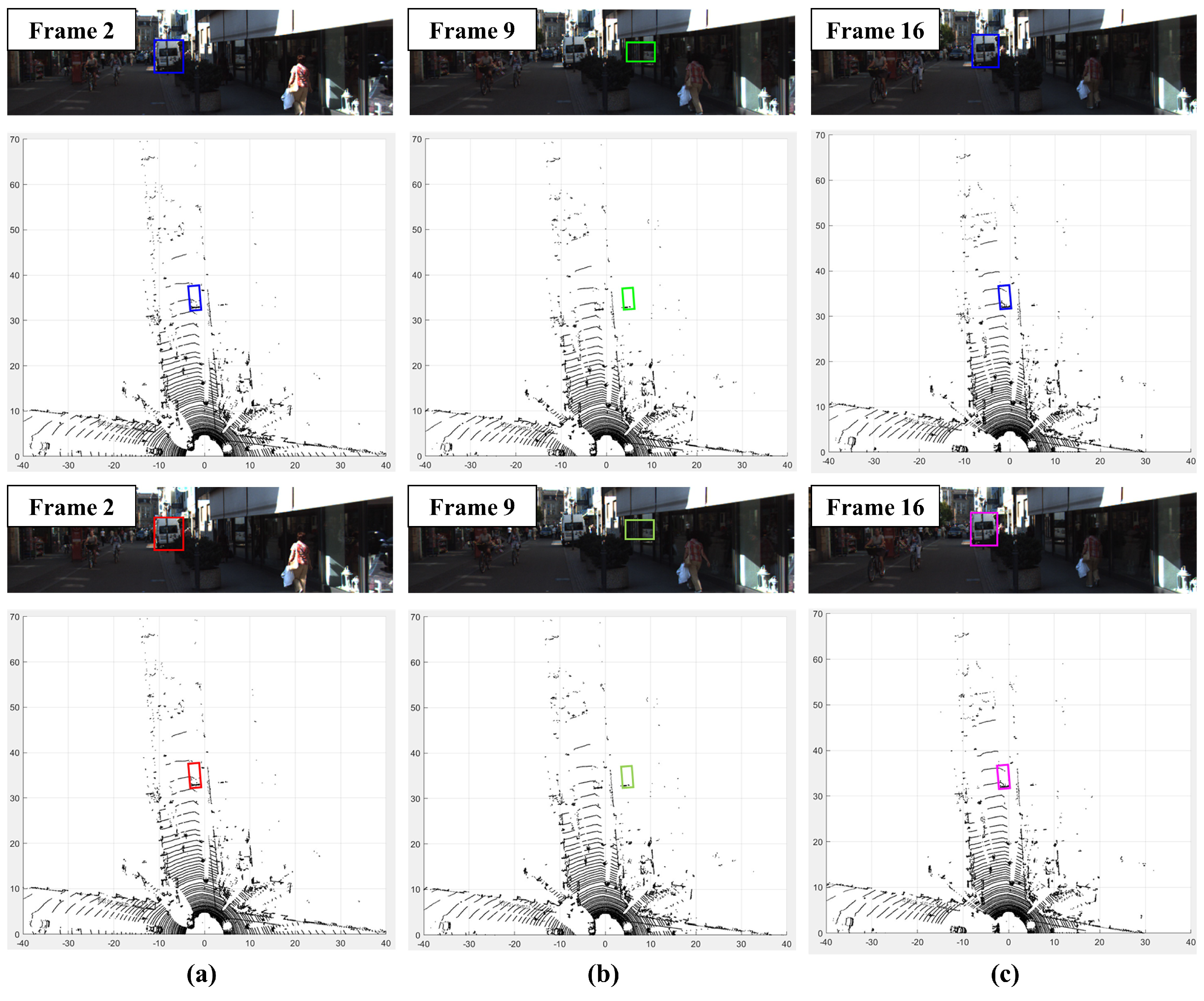
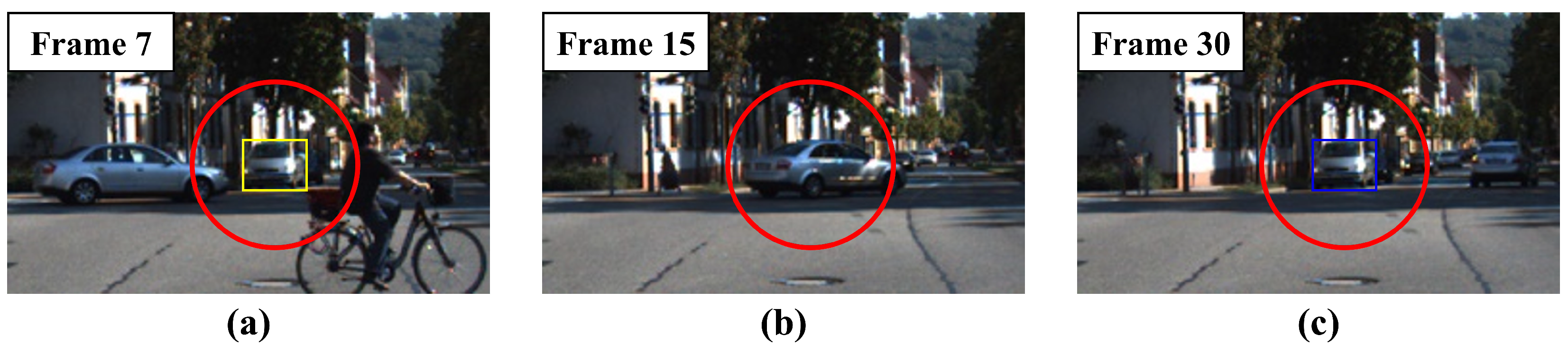
4.4. Qualitative Result

In the field of Multi-Object Tracking, various challenges, including occlusion, present significant difficulties. To assess the effectiveness of the proposed method, a comparative analysis was conducted using the KITTI tracking dataset [47]. In this evaluation, three distinct experimental scenarios were focused on, each highlighting a different aspect of the proposed method’s superiority. These scenarios included instances of short-term occlusion when the ego-vehicle was motionless, occlusion occurring while the ego-vehicle was in motion, and prolonged occlusion when the ego-vehicle was stationary. To provide a visual context for these scenarios, please refer to Figure 9, Figure 10 and Figure 11.

Figure 9 showcases a comparison of the tracking results in a stationary situation of the ego-vehicle (Testing Sequence 0010). In Figure 9, the tracking results obtained from the 3D LiDAR are projected onto the 2D image plane to enhance the visualization, and each color represents a distinct object ID. Figure 9a,b correspond to the results of AB3DMOT [1] and the proposed method, respectively. In Figure 9a,b, the object’s state before, during, and after occlusion is illustrated progressing from left to right, as indicated by the red circle. From Frame 66, it is witnessed that the object experiencing occlusion reappears in Frame 72. This observation highlights a key difference between the proposed method and the existing approach. In the existing method, occlusion persists beyond a predefined threshold, leading to the deletion of the current track information and an associated ID switching event. In contrast, the proposed method temporarily deactivated the target, applying an “inactive” state during occlusion while preserving the track information. Consequently, it can be confirmed that the same ID was re-assigned to the object upon re-detection after occlusion. In essence, the proposed method demonstrated stable tracking without ID switching.

Figure 10 illustrates a scenario in which two stationary vehicles are occluded by another vehicle approaching from the opposite direction, while the ego-vehicle is in forward motion. In the first column of Figure 10, the two vehicles marked in blue are initially detected in Frame 12. As shown in the center column of Figure 10, both vehicles become occluded by the oncoming vehicle in Frame 35. However, in Frame 45, which is 10 frames after the initial occlusion, these two vehicles reappear. Similar to the findings in Figure 9, the existing method assigned new IDs to the two vehicles. In contrast, the proposed method maintained the original IDs for both vehicles when they reappeared. This preservation of IDs was achieved by considering the “inactive” state of each target during occlusion.

Figure 11 depicts a scenario where a moving vehicle becomes occluded by a stationary vehicle at an intersection. In Figure 11a the detection of a vehicle moving from east to west at Frame 95 (assuming the ego vehicle’s location is south) is observed. This vehicle is occluded for approximately 10 frames, reappears at Frame 121, and continues to be tracked until Frame 133 within the sensor’s Field of View (FoV). Figure 11b,c illustrate the trajectory connecting the center coordinates of the tracked object using two different methods: AB3DMOT [1] and the proposed method. Figure 11b displays the results from the previous tracking method, which encounters an issue when tracks are deleted during occlusion. Even if the same object was detected again, it was assigned a new ID. In contrast, the proposed method, as shown in Figure 11c, demonstrated a more-robust tracking approach. It maintained the track during occlusion by utilizing the “inactive” state and continued tracking the object with the same ID. This was achieved by leveraging the Graph-Convolutional-Network (GCN)-based long-term association.

4.5. Ablation Study

In the ablation studies, the KITTI tracking validation dataset was employed to demonstrate the effectiveness of the proposed method.

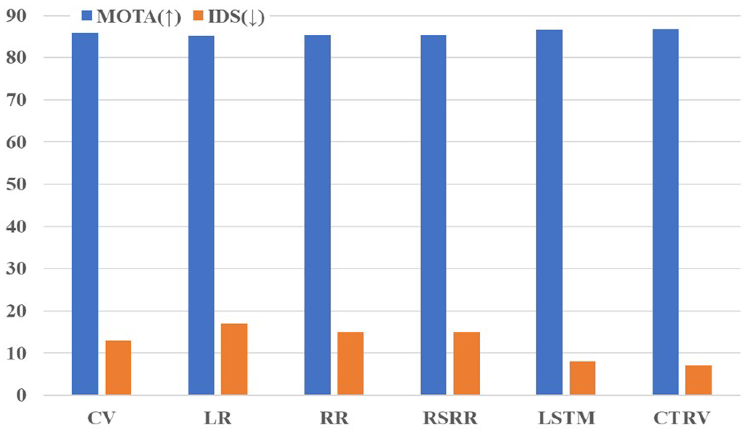
4.5.1. Effectiveness of the Predictor

To validate the effectiveness of the predictor, the tracking performance with the Constant Turn Rate and Velocity (CTRV) model was compared with other predictors. The models included the Constant Velocity (CV), Linear Regression (LR), Ridge Regression (RR), RANSAC with ridge regression, and LSTM models from [56]. These models were applied to predict motion in the proposed method using the KITTI validation set, while keeping all other elements constant. Figure 12 illustrates the result of the MOTA and IDS on the KITTI validation set. In the figure, the blue section represents the MOTA, where a higher value signifies better performance. Conversely, the orange part corresponds to the ID Switches (IDSs), with a lower value indicating better performance. The results indicated a slight improvement of the CTRV model in the MOTA compared to other models. The distinctive feature of the CTRV model lies in its utilization of the target’s heading angle for prediction, unlike the LSTM and CV models, which rely solely on the target’s previous coordinates. Notably, the CTRV model demonstrated similar performance without the need for additional training, offering computational efficiency. This characteristic stems from the assumption that the CTRV model makes predictions based on the vehicle’s motion model.

4.5.2. Effectiveness of Proposed Multi-Level Association

To demonstrate the effectiveness of every component in the proposed multi-level association and track management strategy, each component was separately removed and kept unchanged. As shown in

Table 3. Performance comparison with and without proposed methods on KITTI validation dataset. In the table, “✓” indicates that the part is applied, while “-” denotes that it is not applied. Moreover, “↑” indicates that the higher the value, the better the performance, and “↓” means vice versa. The values showing the best performance for each metric are indicated in bold.

Application			MOTA (↑)	IDS (↓)	FRAG (↓)
Short-Term	Long-Term	Track Management
✓	-	-	85.28%	23	219
✓	✓	-	86.01%	15	142
✓	-	✓	85.84%	18	184
✓	✓	✓	86.79%	7	83

, each component had a positive impact on the proposed tracking method. Comparing the method utilizing only the short-term association with the one incorporating track management by introducing an “inactive” state for the unassociated target, the IDS decreased. Furthermore, it was confirmed that improving tracking performance can be achieved through the implementation of the long-term associations with unmatched targets through the short-term associations. In other words, the proposed strategies, which involve assigning an “inactive” state for an unassociated target and applying the long-term associations, effectively reduced the IDS while enhancing the overall tracking performance.

4.5.3. Tracking Performance with Respect to Target Distance

To investigate the effectiveness of the proposed method, a comparative analysis of the tracking performance results was conducted, specifically focusing on the distance between tracked objects with the existing method, AB3DMOT [1]. As shown in

Table 4. Performance comparison between the proposed method and existing MOT method with respect to target distance on the KITTI validation dataset. In the table, “↑” indicates that the higher the value, the better the performance, and “↓” means vice versa. The values showing the best performance for each metric are indicated in bold.

Method	Distance < 30 m		30 m ≤ Distance ≤ 50 m		Distance > 50 m
	MOTA (↑)	IDS (↓)	MOTA (↑)	IDS (↓)	MOTA (↑)	IDS (↓)
AB3DMOT [1]	86.85%	6	85.27%	9	83.73%	8
Proposed method	88.89%	0	86.35%	5	85.13%	2

, it is apparent that the proposed method consistently outperformed AB3DMOT in tracking, regardless of the target distance. Notably, while an increase in the number of IDSs was experienced by AB3DMOT as the distance from the target grew, fewer IDSs were exhibited, and solid tracking performance was maintained in the proposed method. These results emphasize that, as tracking based solely on the IoU became less effective for distant targets, robust tracking was ensured by utilizing the long-term association with the target’s path as proposed.

4.5.4. Tracking Performance with False Detection

To demonstrate the robustness of the proposed method against false detections, a qualitative study was conducted, focusing on scenarios in which false detections might occur within a road environment. Within various road scenarios, false detections can occasionally be attributed to the reflection of the LiDAR point cloud by a large piece of glass along the street. Figure 13 depicts a scenario in which false detection took place near a large piece of glass in the street. In Figure 13, the upper line and lower line correspond to the proposed method’s and AB3DMOT’s tracking results, respectively. As shown in Figure 13b, the false detection occurred due to the reflected point cloud on the glass. The proposed method initialized the falsely detected object in Figure 13b as a new track, but managed the tracked object in Figure 13a as an “inactive track”. Consequently, when the vehicle was re-detected, as depicted in Figure 13c, it could be assigned the same ID as in Figure 13a. On the contrary, the AB3DMOT method removed the target information in Frame 2 that had not been associated for a long time. Therefore, even if the same vehicle was re-detected after a false detection, it was allocated a different ID than before. In summary, though tracking performance may be impaired by false detections near large pieces of glass, stable tracking can be achieved through the application of the proposed multi-level association and track management.

5. Conclusions

In this paper, a robust Multi-Object Tracking (MOT) framework tailored for 3D LiDAR data was introduced, with a specific focus on meeting the demands of intelligent transportation systems and Autonomous Driving Assistance Systems (ADASs). The proposed approach incorporates a multi-level association technique that effectively mitigates challenges such as ID switching after occlusion, and it introduces an innovative association method utilizing Graph Convolutional Networks (GCNs) to evaluate the vehicle trajectories. The comparative analysis with the state-of-the-art LiDAR and LiDAR–camera fusion tracking methods demonstrated the clear effectiveness of the proposed approach in enhancing robustness, particularly in addressing ID switching and fragment problems. The proposed method was examined using the KITTI benchmark MOT tracking dataset and attained a HOTA of 75.65%, representing a 5.66% enhancement compared to the benchmark method, AB3DMOT. Moreover, it significantly reduced the number of ID switches to 39, 74 fewer than AB3DMOT. These outcomes provide strong validation for the effectiveness of the proposed approach across various road environments. In future work, the strategy to robustly detect occluded objects through completion will be studied as a pre-processing step. Moreover, the management of the “inactive” state will be enhanced, such as by using reinforcement learning, or the proposed single-vehicle-centric tracking will be developed for its application in a connected automated vehicle-based MOT method.

References

1. Weng, X.; Wang, J.; Held, D.; Kitani, K. 3D Multi-Object Tracking: A baseline and new evaluation metrics. In Proceedings of the 2020 IEEE/RSJ International Conference on Intelligent Robots and Systems (IROS), Las Vegas, NV, USA, 25–29 October 2020; pp. 10359–10366. [Google Scholar]
2. Yin, T.; Zhou, X.; Krahenbuhl, P. Center-based 3D object detection and tracking. In Proceedings of the IEEE/CVF Conference on Computer Vision and Pattern Recognition, Nashville, TN, USA, 20–25 June 2021; pp. 11784–11793. [Google Scholar]
3. Chiu, H.; Prioletti, A.; Li, J.; Bohg, J. Probabilistic 3D Multi-Object Tracking for autonomous driving. arXiv 2020, arXiv:2001.05673. [Google Scholar]
4. Liu, H.; Ma, Y.; Hu, Q.; Guo, Y. CenterTube: Tracking Multiple 3D Objects with 4D Tubelets in Dynamic Point Clouds. IEEE Trans. Multimed. 2023; early access. [Google Scholar]
5. Du, Y.; Zhao, Z.; Song, Y.; Zhao, Y.; Su, F.; Gong, T.; Meng, H. Strongsort: Make deepsort great again. IEEE Trans. Multimed. 2023; early access. [Google Scholar]
6. Zhang, Y.; Sun, P.; Jiang, Y.; Yu, D.; Weng, F.; Yuan, Z.; Luo, P.; Liu, W.; Wang, X. Bytetrack: Multi-object tracking by associating every detection box. In Proceedings of the Computer Vision—ECCV 2022: 17th European Conference, Tel Aviv, Israel, 23–27 October 2022; Proceedings, Part XXII. Springer: Berlin/Heidelberg, Germany, 2022; pp. 1–21. [Google Scholar]
7. Cao, J.; Pang, J.; Weng, X.; Khirodkar, R.; Kitani, K. Observation-centric sort: Rethinking sort for robust Multi-Object Tracking. In Proceedings of the IEEE/CVF Conference on Computer Vision and Pattern Recognition, Vancouver, BC, Canada, 17–24 June 2023; pp. 9686–9696. [Google Scholar]
8. Kim, A.; Ošep, A.; Leal-Taixé, L. Eagermot: 3D Multi-Object Tracking via sensor fusion. In Proceedings of the 2021 IEEE International Conference on Robotics and Automation (ICRA), Xi’an, China, 30 May–5 June 2021; pp. 11315–11321. [Google Scholar]
9. Huang, K.; Hao, Q. Joint multi-object detection and tracking with camera-LiDAR fusion for autonomous driving. In Proceedings of the 2021 IEEE/RSJ International Conference on Intelligent Robots and Systems (IROS), Prague, Czech Republic, 27 September–1 October 2021; pp. 6983–6989. [Google Scholar]
10. Wang, X.; Fu, C.; Li, Z.; Lai, Y.; He, J. DeepFusionMOT: A 3D Multi-Object Tracking Framework Based on Camera-LiDAR Fusion with Deep Association. IEEE Robot. Autom. Lett. 2022, 7, 8260–8267. [Google Scholar] [CrossRef]
11. Cheng, X.; Zhou, J.; Liu, P.; Zhao, X.; Wang, H. 3D Vehicle Object Tracking Algorithm Based on Bounding Box Similarity Measurement. IEEE Trans. Intell. Transp. Syst. 2023; early access. [Google Scholar]
12. Kim, A.; Brasó, G.; Ošep, A.; Leal-Taixé, L. PolarMOT: How far can geometric relations take us in 3D Multi-Object Tracking? In Proceedings of the Computer Vision—ECCV 2022: 17th European Conference, Tel Aviv, Israel, 23–27 October 2022; Proceedings, Part XXII. Springer: Berlin/Heidelberg, Germany, 2022; pp. 41–58. [Google Scholar]
13. Wu, H.; Li, Q.; Wen, C.; Li, X.; Fan, X.; Wang, C. Tracklet Proposal Network for Multi-Object Tracking on Point Clouds. In Proceedings of the International Joint Conference on Artificial Intelligence, Montreal, QC, Canada, 19–27 August 2021; pp. 1165–1171. [Google Scholar]
14. Luo, W.; Yang, B.; Urtasun, R. Fast and furious: Real-time end-to-end 3D detection, tracking and motion forecasting with a single convolutional net. In Proceedings of the IEEE Conference on Computer Vision and Pattern Recognition, Salt Lake City, UT, USA, 18–23 June 2018; pp. 3569–3577. [Google Scholar]
15. Chang, M.; Lambert, J.; Sangkloy, P.; Singh, J.; Bak, S.; Hartnett, A.; Wang, D.; Carr, P.; Lucey, S.; Ramanan, D.; et al. Argoverse: 3D tracking and forecasting with rich maps. In Proceedings of the IEEE/CVF Conference on Computer Vision and Pattern Recognition, Long Beach, CA, USA, 15–20 June 2019; pp. 8748–8757. [Google Scholar]
16. Dai, P.; Weng, R.; Choi, W.; Zhang, C.; He, Z.; Ding, W. Learning a proposal classifier for multiple object tracking. In Proceedings of the IEEE/CVF Conference on Computer Vision and Pattern Recognition, Nashville, TN, USA, 20–25 June 2021; pp. 2443–2452. [Google Scholar]
17. Gharineiat, Z.; Tarsha Kurdi, F.; Campbell, G. Review of automatic processing of topography and surface feature identification LiDAR data using machine learning techniques. Remote Sens. 2022, 14, 4685. [Google Scholar] [CrossRef]
18. Solares-Canal, A.; Alonso, L.; Picos, J.; Armesto, J. Automatic tree detection and attribute characterization using portable terrestrial lidar. Trees 2023, 37, 963–979. [Google Scholar] [CrossRef]
19. Kim, B.; Choi, B.; Park, S.; Kim, H.; Kim, E. Pedestrian/vehicle detection using a 2.5-D multi-layer laser scanner. IEEE Sens. J. 2015, 16, 400–408. [Google Scholar] [CrossRef]
20. Shi, S.; Wang, X.; Li, H. Pointrcnn: 3D object proposal generation and detection from point cloud. In Proceedings of the IEEE/CVF Conference on Computer Vision and Pattern Recognition, Long Beach, CA, USA, 15–20 June 2019; pp. 770–779. [Google Scholar]
21. Shi, S.; Guo, C.; Jiang, L.; Wang, Z.; Shi, J.; Wang, X.; Li, H. Pv-rcnn: Point-voxel feature set abstraction for 3D object detection. In Proceedings of the IEEE/CVF Conference on Computer Vision and Pattern Recognition, Seattle, WA, USA, 13–19 June 2020; pp. 10529–10538. [Google Scholar]
22. Zhou, C.; Zhang, Y.; Chen, J.; Huang, D. OcTr: Octree-based Transformer for 3D Object Detection. In Proceedings of the IEEE/CVF Conference on Computer Vision and Pattern Recognition, Vancouver, BC, Canada, 17–24 June 2023; pp. 5166–5175. [Google Scholar]
23. Wu, H.; Wen, C.; Shi, S.; Li, X.; Wang, C. Virtual Sparse Convolution for Multimodal 3D Object Detection. In Proceedings of the IEEE/CVF Conference on Computer Vision and Pattern Recognition, Vancouver, BC, Canada, 17–24 June 2023; pp. 21653–21662. [Google Scholar]
24. Chen, X.; Li, S.; Mersch, B.; Wiesmann, L.; Gall, J.; Behley, J.; Stachniss, C. Moving object segmentation in 3D LiDAR data: A learning-based approach exploiting sequential data. IEEE Robot. Autom. Lett. 2021, 6, 6529–6536. [Google Scholar] [CrossRef]
25. Wang, S.; Zhu, J.; Zhang, R. Meta-rangeseg: Lidar sequence semantic segmentation using multiple feature aggregation. IEEE Robot. Autom. Lett. 2022, 7, 9739–9746. [Google Scholar] [CrossRef]
26. Marcuzzi, R.; Nunes, L.; Wiesmann, L.; Behley, J.; Stachniss, C. Mask-based panoptic lidar segmentation for autonomous driving. IEEE Robot. Autom. Lett. 2023, 8, 1141–1148. [Google Scholar] [CrossRef]
27. Xia, Y.; Xu, Y.; Wang, C.; Stilla, U. VPC-Net: Completion of 3D vehicles from MLS point clouds. ISPRS J. Photogramm. Remote Sens. 2021, 174, 166–181. [Google Scholar] [CrossRef]
28. Zheng, C.; Yan, X.; Zhang, H.; Wang, B.; Cheng, S.; Cui, S.; Li, Z. Beyond 3D siamese tracking: A motion-centric paradigm for 3D single object tracking in point clouds. In Proceedings of the IEEE/CVF Conference on Computer Vision and Pattern Recognition, New Orleans, LA, USA, 18–24 June 2022; pp. 8111–8120. [Google Scholar]
29. Wang, P.; Ren, L.; Wu, S.; Yang, J.; Yu, E.; Yu, H.; Li, X. Implicit and Efficient Point Cloud Completion for 3D Single Object Tracking. IEEE Robot. Autom. Lett. 2023, 8, 1935–1942. [Google Scholar] [CrossRef]
30. Cui, Y.; Xu, H.; Wu, J.; Sun, Y.; Zhao, J. Automatic vehicle tracking with roadside LiDAR data for the connected-vehicles system. IEEE Intell. Syst. 2019, 34, 44–51. [Google Scholar] [CrossRef]
31. Meng, Z.; Xia, X.; Xu, R.; Liu, W.; Ma, J. HYDRO-3D: Hybrid Object Detection and Tracking for Cooperative Perception Using 3D LiDAR. IEEE Trans. Intell. Transp. Syst. 2023; early access. [Google Scholar]
32. Yu, H.; Luo, Y.; Shu, M.; Huo, Y.; Yang, Z.; Shi, Y.; Guo, Z.; Li, H.; Hu, X.; Yuan, J.; et al. Dair-v2x: A large-scale dataset for vehicle-infrastructure cooperative 3D object detection. In Proceedings of the IEEE/CVF Conference on Computer Vision and Pattern Recognition, New Orleans, LA, USA, 18–24 June 2022; pp. 21361–21370. [Google Scholar]
33. Xu, R.; Xia, X.; Li, J.; Li, H.; Zhang, S.; Tu, Z.; Meng, Z.; Xiang, H.; Dong, X.; Song, R.; et al. V2v4real: A real-world large-scale dataset for vehicle-to-vehicle cooperative perception. In Proceedings of the IEEE/CVF Conference on Computer Vision and Pattern Recognition, Vancouver, BC, Canada, 17–24 June 2023; pp. 13712–13722. [Google Scholar]
34. Guo, G.; Zhao, S. 3D Multi-Object Tracking with adaptive cubature Kalman filter for autonomous driving. IEEE Trans. Intell. Veh. 2022, 8, 512–519. [Google Scholar] [CrossRef]
35. Wu, H.; Han, W.; Wen, C.; Li, X.; Wang, C. 3D Multi-Object Tracking in point clouds based on prediction confidence-guided data association. IEEE Trans. Intell. Transp. Syst. 2021, 23, 5668–5677. [Google Scholar] [CrossRef]
36. Shenoi, A.; Patel, M.; Gwak, J.; Goebel, P.; Sadeghian, A.; Rezatofighi, H.; Martin-Martin, R.; Savarese, S. Jrmot: A real-time 3D multi-object tracker and a new large-scale dataset. In Proceedings of the 2020 IEEE/RSJ International Conference on Intelligent Robots and Systems (IROS), Las Vegas, NV, USA, 25–29 October 2020; pp. 10335–10342. [Google Scholar]
37. Brasó, G.; Leal-Taixé, L. Learning a neural solver for multiple object tracking. In Proceedings of the IEEE/CVF Conference on Computer Vision and Pattern Recognition, Seattle, WA, USA, 13–19 June 2020; pp. 6247–6257. [Google Scholar]
38. Li, J.; Gao, X.; Jiang, T. Graph networks for multiple object tracking. In Proceedings of the IEEE/CVF Winter Conference on Applications of Computer Vision, Snowmass Village, CO, USA, 1–5 March 2020; pp. 719–728. [Google Scholar]
39. Weng, X.; Wang, Y.; Man, Y.; Kitani, K. Gnn3dmot: Graph neural network for 3D Multi-Object Tracking with 2D-3D multi-feature learning. In Proceedings of the IEEE/CVF Conference on Computer Vision and Pattern Recognition, Seattle, WA, USA, 13–19 June 2020; pp. 6499–6508. [Google Scholar]
40. He, J.; Huang, Z.; Wang, N.; Zhang, Z. Learnable graph matching: Incorporating graph partitioning with deep feature learning for multiple object tracking. In Proceedings of the IEEE/CVF Conference on Computer Vision and Pattern Recognition, Nashville, TN, USA, 20–25 June 2021; pp. 5299–5309. [Google Scholar]
41. Zhai, G.; Meng, H.; Wang, X. A constant speed changing rate and constant turn rate model for maneuvering target tracking. Sensors 2014, 14, 5239–5253. [Google Scholar] [CrossRef] [PubMed]
42. Ondruska, P.; Posner, I. Deep tracking: Seeing beyond seeing using recurrent neural networks. In Proceedings of the AAAI Conference on Artificial Intelligence, Phoenix, AZ, USA, 12–17 February 2016; Volume 30. [Google Scholar]
43. Milan, A.; Rezatofighi, S.; Dick, A.; Reid, I.; Schindler, K. Online multi-target tracking using recurrent neural networks. In Proceedings of the AAAI Conference on Artificial Intelligence, San Francisco, CA, USA, 4–9 February 2017; Volume 31. [Google Scholar]
44. Xiang, J.; Zhang, G.; Hou, J. Online Multi-Object Tracking based on feature representation and Bayesian filtering within a deep learning architecture. IEEE Access 2019, 7, 27923–27935. [Google Scholar] [CrossRef]
45. Hu, H.; Cai, Q.; Wang, D.; Lin, J.; Sun, M.; Krahenbuhl, P.; Darrell, T.; Yu, F. Joint monocular 3D vehicle detection and tracking. In Proceedings of the IEEE/CVF International Conference on Computer Vision, Seoul, Republic of Korea, 27 October–2 November 2019; pp. 5390–5399. [Google Scholar]
46. Kuhn, H. The Hungarian method for the assignment problem. Nav. Res. Logist. (NRL) 2005, 52, 7–21. [Google Scholar] [CrossRef]
47. Geiger, A.; Lenz, P.; Urtasun, R. Are we ready for autonomous driving? The kitti vision benchmark suite. In Proceedings of the 2012 IEEE Conference on Computer Vision and Pattern Recognition, Providence, RI, USA, 16–21 June 2012; pp. 3354–3361. [Google Scholar]
48. Bernardin, K.; Stiefelhagen, R. Evaluating multiple object tracking performance: The clear mot metrics. EURASIP J. Image Video Process. 2008, 2008, 246309. [Google Scholar] [CrossRef]
49. Luiten, J.; Osep, A.; Dendorfer, P.; Torr, P.; Geiger, A.; Leal-Taixé, L.; Leibe, B. Hota: A higher order metric for evaluating Multi-Object Tracking. Int. J. Comput. Vis. 2021, 129, 548–578. [Google Scholar] [CrossRef]
50. Wang, S.; Sun, Y.; Liu, C.; Liu, M. Pointtracknet: An end-to-end network for 3-d object detection and tracking from point clouds. IEEE Robot. Autom. Lett. 2020, 5, 3206–3212. [Google Scholar] [CrossRef]
51. Wang, S.; Cai, P.; Wang, L.; Liu, M. Ditnet: End-to-end 3D object detection and track id assignment in spatio-temporal world. IEEE Robot. Autom. Lett. 2021, 6, 3397–3404. [Google Scholar] [CrossRef]
52. Luiten, J.; Fischer, T.; Leibe, B. Track to reconstruct and reconstruct to track. IEEE Robot. Autom. Lett. 2020, 5, 1803–1810. [Google Scholar] [CrossRef]
53. Jiang, C.; Wang, Z.; Liang, H.; Tan, S. A fast and high-performance object proposal method for vision sensors: Application to object detection. IEEE Sens. J. 2022, 22, 9543–9557. [Google Scholar] [CrossRef]
54. Zhang, K.; Liu, Y.; Mei, F.; Jin, J.; Wang, Y. Boost Correlation Features with 3D-MiIoU-Based Camera-LiDAR Fusion for MODT in Autonomous Driving. Remote Sens. 2023, 15, 874. [Google Scholar] [CrossRef]
55. Wang, X.; Fu, C.; He, J.; Wang, S.; Wang, J. StrongFusionMOT: A Multi-Object Tracking Method Based on LiDAR-Camera Fusion. IEEE Sens. J. 2022, 23, 11241–11252. [Google Scholar] [CrossRef]
56. Xia, Y.; Wu, Q.; Li, W.; Chan, A.; Stilla, U. A Lightweight and Detector-Free 3D Single Object Tracker on Point Clouds. IEEE Trans. Intell. Transp. Syst. 2023, 24, 5543–5554. [Google Scholar] [CrossRef]
Figure 1. An example of ID switching due to occlusion. In (a,c), the color of each box indicates the ID of each target. (a) There is a vehicle with its ID. (b) Another vehicle turns at the intersection, occluding that vehicle for about 8 frames. After occlusion, the ID given in (a) is changed in (c).
Remotesensing 15 05486 g001
Figure 2. The flowchart for the proposed method.
Remotesensing 15 05486 g002
Figure 3. The architecture of the proposed method. All procedures are performed in the 3D LiDAR domain, and the results on 2D images are used only for reference of the visualization by projecting the 3D results. The inputs of association are X ^ t , the prediction of time t by using previous tracked state X t 1 , and D t , the detection of time t. After short-term and long-term association, the target states are updated with the condition including whether they are associated, occluded, or deleted. The red and blue boxes denote the active and the inactive (occluded or disappeared) tracks, respectively.
Remotesensing 15 05486 g003
Figure 4. (a) Situation when the 1st association failed. (b) Trajectories before and after occlusion in the situation of (a). The red and blue trajectory represents the trajectory before occlusion and after reappearing, respectively.
Remotesensing 15 05486 g004
Figure 5. An example of the input and situation for the proposed 2nd association. In the figure, D ¯ t 1 and X ¯ ^ t 2 are the input of the 2nd association because D t 2 and T t 1 1 are matched by the 1st association and updated as T t 1 T t 1 1 { D t 2 } .
Remotesensing 15 05486 g005
Figure 6. An example of Tr t j . In this figure, the jth track was initialized time t j ago and tracked until time t − 1. The predicted position of this track at time t is denoted as ( x ^ , y ^ ) t j , but it was assumed that this track does not match any detections from the 1st association. In this case, the trajectory Tr t j is generated by connecting all target locations except the predicted state.
Remotesensing 15 05486 g006
Figure 7. Illustration of 2nd-association-based long-term relation.
Remotesensing 15 05486 g007
Figure 8. The real data example of robust tracking using long-term association. (a) The situation before and after the occlusion (the cyan vehicle in Frame 95 and the blue vehicle in Frame 141 are the same object). (b) The situation of Frame 141 in the LiDAR domain. (c) Enlarged view of the area indicated in (b). Point A is the predicted location of the X ¯ ^ t A . (d,e) are the generated graph by connecting the detection (Objects B and C in (c)) and the track marked as cyan color in (c).
Remotesensing 15 05486 g008
Figure 9. Qualitativeresult for Testing Set Sequence 0010, with the ego-vehicle stationary. This figure demonstrates a scenario where a stopped vehicle is occluded by another vehicle turning at the intersection and reappearing. Each color represents a distinct object ID.
Remotesensing 15 05486 g009
Figure 10. Qualitative result for Testing Set Sequence 0018, with the ego-vehicle in motion. This figure illustrates a scenario where two stationary vehicles are occluded by another vehicle approaching from the opposite direction while the ego-vehicle continues moving forward.
Remotesensing 15 05486 g010
Figure 11. Qualitative results for Testing Set Sequence 0013. This figure compares the tracking results using the GCN-based long-term relation approach. In (a), the situation before and after the occlusion of the target is illustrated. The left and right column show the tracking results using AB3DMOT and the proposed method, respectively. Frame 95 features a red vehicle, and Frames 121 and 133 depict a blue vehicle, all referring to the same object. Unlike existing tracking methods, which often encounter ID switching problems, the proposed method maintained consistent IDs assigned to objects. (b,c) present the trajectory-based tracking results transformed and projected into the Bird’s-Eye View (BEV). Specifically, (b) illustrates the results from the existing tracking method, while (c) showcases the tracking results achieved by the proposed method, highlighting its effectiveness.
Remotesensing 15 05486 g011
Figure 12. Comparison of prediction models with the CTRV model on the KITTI validation set.
Remotesensing 15 05486 g012
Figure 13. False detection situations occur near a large piece of glass. The upper line and lower line of the figure correspond to the proposed method’s and AB3DMOT’s tracking results, respectively. In (b), the false detection occurs due to the reflection of the point cloud on the glass, (a,c) represent the tracking results before and after false detection, respectively. As depicted in the figures, the proposed method maintains the same ID for the object re-detected after false detection, thanks to the "inactive state". In contrast, AB3DMOT assigns a different ID to that object since the track information before false detection is deleted.
Remotesensing 15 05486 g013