Is Spectral Unmixing Model or Nonlinear Statistical Model More Suitable for Shrub Coverage Estimation in Shrub-Encroached Grasslands Based on Earth Observation Data? A Case Study in Xilingol Grassland, China

Abstract

Due to the effects of global climate change and altered human land-use patterns, typical shrub encroachment in grasslands has become one of the most prominent ecological problems in grassland ecosystems. Shrub coverage can quantitatively indicate the degree of shrub encroachment in grasslands; therefore, real-time and accurate monitoring of shrub coverage in large areas has important scientific significance for the protection and restoration of grassland ecosystems. As shrub-encroached grasslands (SEGs) are a type of grassland with continuous and alternating growth of shrubs and grasses, estimating shrub coverage is different from estimating vegetation coverage. It is not only necessary to consider the differences in the characteristics of vegetation and non-vegetation variables but also the differences in characteristics of shrubs and herbs, which can be a challenging estimation. There is a scientific need to estimate shrub coverage in SEGs to improve our understanding of the process of shrub encroachment in grasslands. This article discusses the spectral differences between herbs and shrubs and further points out the possibility of distinguishing between herbs and shrubs. We use Sentinel-2 and Gao Fen-6 (GF-6) Wide Field of View (WFV) as data sources to build a linear spectral mixture model and a random forest (RF) model via space–air–ground collaboration and investigate the effectiveness of different data sources, features and methods in estimating shrub coverage in SEGs, which provide promising ways to monitor the dynamics of SEGs. The results showed that (1) the linear spectral mixture model can hardly distinguish between shrubs and herbs from medium-resolution images in the SEG. (2) The RF model showed high estimation accuracy for shrub coverage in the SEG; the estimation accuracy (R²) of the Sentinel-2 image was 0.81, and the root-mean-square error (RMSE) was 0.03. The R² of the GF6-WFV image was 0.72, and the RMSE was 0.03. (3) Texture feature introduced in RF models are helpful to estimate shrub coverage in SEGs. (4) Regardless of the linear spectral mixture model or the RF model being employed, the Sentinel-2 image presented a better estimation than the GF6-WFV image; thus, this data has great potential to monitor shrub encroachment in grasslands. This research aims to provide a scientific basis and reference for remote sensing-based monitoring of SEGs.

1. Introduction

Fractional vegetation cover is a direct quantitative indicator reflecting the growth status of vegetation; it is an important parameter for estimating and monitoring the physical and chemical characteristics of vegetation [1,2]. In recent decades, due to factors such as climate change and human-induced alterations in land-use patterns, grasslands in the arid and semi-arid areas of Inner Mongolia, China, have gradually degraded, causing shrub vegetation to expand over large areas. On the grassland substrate, patches of shrub vegetation have gradually formed, which is known as shrub-encroached grasslands (SEGs) [3,4,5,6]. At present, there are 5.1 million hectares of SEGs of Caragana microphylia in Inner Mongolia [7]. With further increase in shrub vegetation, the species composition of the original grassland ecosystem and the competition between shrub and herbaceous vegetation for nutrients will change. This is expected to significantly affect the structure and function of the entire ecosystem in arid and semi-arid regions. Shrub coverage quantitatively represents the degree of shrub encroachment in grasslands [8]. Therefore, accurate, real-time, and large-scale estimation of shrub coverage in SEGs is of great significance for the protection and restoration of the original ecosystem in SEGs.

Traditional methods to measure shrub coverage entail field measurements, such as the needling method [9], which not only requires a large amount of manpower and material resources, but also has slow investigation speed and can cause certain damage to vegetation. Additionally, it cannot estimate shrub coverage on a large scale, and thus poses many limitations to feasible application. With the continuous development of remote sensing technology, the use of multispectral and hyperspectral remote sensing imaging has opened the possibility of real-time and large-scale measurement of shrub coverage. At the same time, remote sensing with unmanned aerial vehicles (UAVs) serves as a bridge between aerospace remote sensing and ground surveys, providing a large number of samples for constructing vegetation coverage estimation models [10]. In recent years, many studies have used drone aerial images to construct vegetation coverage estimation models [11,12,13,14]. Liu et al. [15] used DJI drones to obtain large sample data for the Hulunbuir Grassland; they estimated vegetation coverage using maximum entropy and genetic algorithms and validated their findings with ground survey data, which indicated high estimation accuracy. This method can yield large volumes of ground validation data for remote sensing-based estimation of shrub coverage. The most commonly available remote sensing images on the market are medium-resolution multispectral images that are prone to spectral mixing and other issues. Therefore, scholars may choose to use mixed spectral decomposition models to estimate vegetation coverage. Cao et al. [16] estimated shrub coverage in the Mu Us Sandland of Wushen Banner, Inner Mongolia. They used spectral mixing models and linear regression models with HJ-1B images for shrub coverage estimation. The results showed that the spectral mixing model performed better than linear regression models. Yang et al. [17] used Landsat TM data to analyze the relationship between different components obtained from mixed spectral models and vegetation coverage. The results from their study indicated that it is feasible to estimate the coverage of desert grasslands using a linear spectral mixing model, especially for the mixed pixels. Liu et al. [18] used the Landsat OLI image data to study Xianghuang Banner, Inner Mongolia; they employed the multiple endmember spectral mixture analysis and linear models integrating shrub phenological characteristics to estimate shrub coverage in SEGs. The results indicated certain spectra differences in shrub and herbaceous vegetation in SEGs; the differences make the identification between them possible. Currently, machine learning methods have achieved good results in estimating vegetation coverage [19,20]. Yang et al. [21] considered the Baiyangdian-Daqinghe Basin as their research object; they combined multi-source data, such as Sentinel-2, Sentinel-1, and DEM, to achieve vegetation coverage inversion based on the random forest regression model method. The results showed that as compared with the inversion results extracted with traditional NDVI pixel dichotomy, the accuracy of vegetation coverage estimated via the random forest regression model was higher. Ge et al. [22] estimated vegetation coverage in alpine areas using support vector regression (SVR) algorithms based on MODIS data. The results showed that the SVR models monitoring the study area based on nine factors performed best, with R² = 0.75 and RMSE = 6.85%, in alpine grassland cover. Previous research focused more on the distinguishability between herbaceous and bare soil and paid less attention to the distinguishability between different vegetation types. However, in SEGs, spectral heterogeneity between different vegetation types needs to be considered. Therefore, the feasibility of spectral mixing models and machine learning methods estimate for shrub coverage estimate under different shrub coverage levels are needed to be further explored.

Sentinel-2 and GF6-WFV have certain applications in vegetation coverage estimation [23,24,25,26]. Compared to other low-resolution satellites, Sentinel-2 and GF6-WFV have higher spatial resolution and band characteristics, which help distinguish between shrubs and herbs. Additionally, Sentinel-2 and GF6-WFV are easier to obtain and have a shorter revisit period, avoiding time errors caused by inconsistent sample and image acquisition times. When facing interference from clouds and mist, it is also easier to obtain images of similar time periods to replace them. Based on these factors, this study uses remote sensing images from UAVs to obtain shrub coverage as ground verification data, extracted band reflectance, vegetation index and texture features using Sentinel-2 and GF6-WFV remote sensing image data. By establishing a spectral mixture model and a random forest model through space–air–ground collaboration approach, the accuracy of these models was compared and analyzed across different coverage levels. Ultimately, the optimal model for estimating shrub coverage was determined via remote sensing. The overall goal of these efforts was to provide a theoretical and practical basis for large-scale, real-time monitoring of SEGs, and sustainable utilization of grassland resources in the local area.

2. Materials and Methods

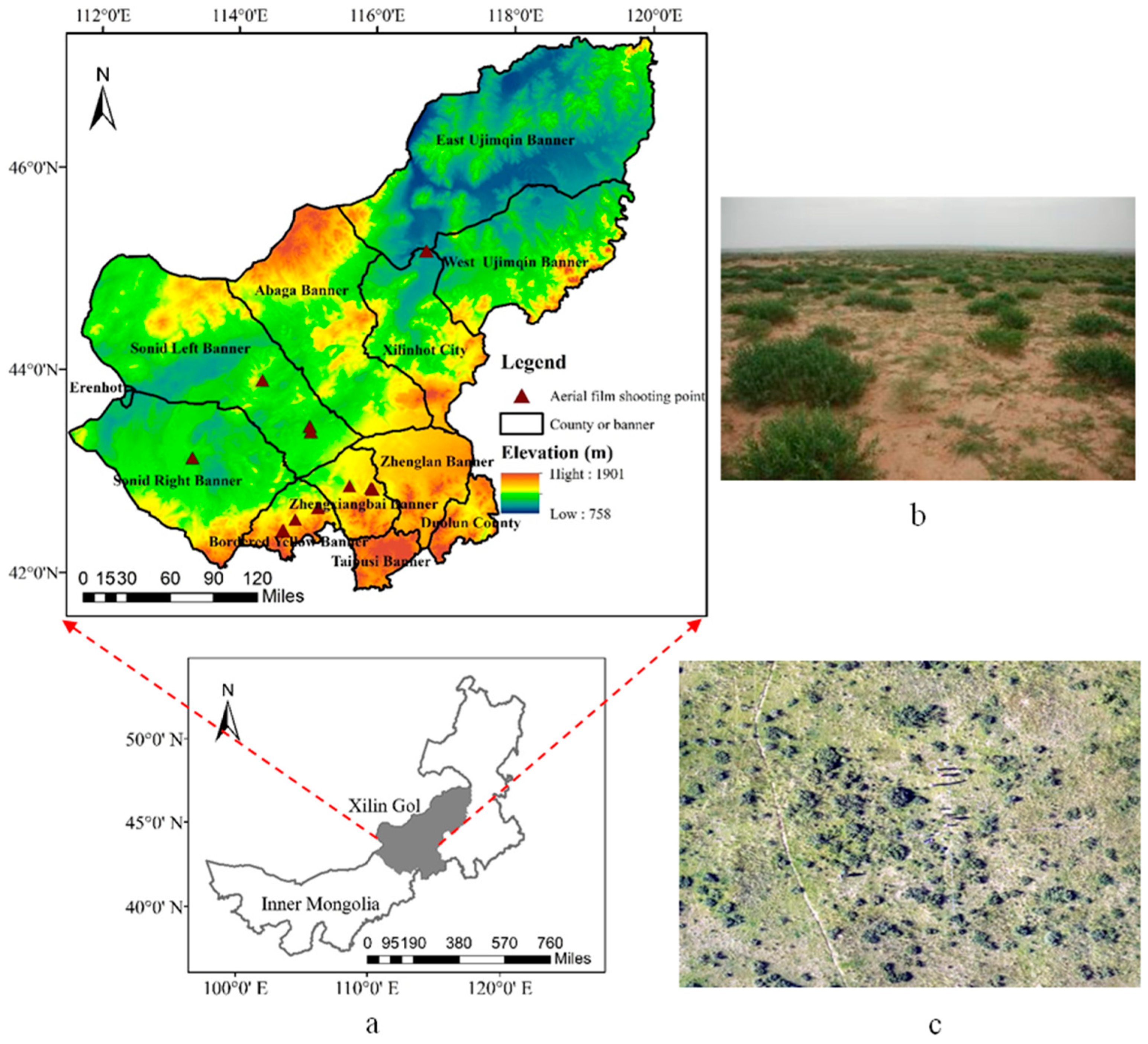
2.1. Study Area

Xilingol is in the middle of Inner Mongolia (41°35′–46°46′N, 111°09′–120°01′E). It borders Mongolia in the north with a 1098 km long borderline. It is adjacent to the Hebei Province in the south, and Chifeng, Hinggan League, and Tongliao in the east. Its grassland area accounts for approximately 176,000 km² [27,28,29] (Figure 1). The terrain of Xilingol is dominated by high plains; the terrain is high in the south and low in the north, and the height above mean sea level is approximately 1000 m. The climate type belongs to the arid and semi-arid continental climate in the middle temperate zone. The annual average temperature is 0–4 °C, and the annual average precipitation is 150–400 mm, decreasing from southeast to northwest [30]. The natural grassland in this area mainly consists of Stipa capillata, Artemisia frigida, Cleistogenes squarrosa, and Allium bidentatum as the dominant species; the main tree species are Ulmus pumila; shrubs are dominated by Caragana microphylia, which is mainly distributed in Zhengxiangbai Banner and Xianghuang Banner. With the increase in shrub coverage, the grassland in this area gradually deteriorates and results in significant ecological protection pressure.

2.2. Field Survey Data

2.2.1. Spectral Data Measurements

This study used the ASD FieldSpec Pro FR 2500 Spectrometer (The equipment comes from Analytica Spectra Devices in the United States) from 26 July to 13 August 2022 to obtain the spectral endmember of specific bare soil, shrub vegetation, herbaceous vegetation, and shadows for each sample plot. The instrument collected spectra in the wavelength range of 350–2500 nm, totaling 2150 wavebands. To prevent the influence of different solar zenith angles on reflectivity and ensure sufficient sunlight, the time period with clear weather and low wind force shall be selected for spectrum measurement (10:00–14:00). The main steps were as follows: the probe was placed on various typical ground objects of interest (such as Caragana microphylla shrub vegetation, herb vegetation, quicksand, and shadow) in each sample plot, and spectra were collected downward at 0.1–0.2 m close to its surface [31]. To ensure the representativeness and applicability of spectral endmembers in the study area, their number should not be less than 10 as frequently as possible. In the end, a total of 47 spectra of shrub vegetation, 45 spectra of herbaceous vegetation, 22 spectra of bare soil, and 10 spectra of shadow were obtained.

2.2.2. Shrub Coverage Data

In this study, shrub coverage was measured through drone imagery (from 26 July to 13 August 2022). The drone model was the DJI Phantom 4 Multispectral (P4M), which is equipped with a multispectral sensor independently produced by the DJI Company, FC6360, with effective pixels of 2.08 million. It can obtain five multispectral bands at once, namely blue, green, red, red edge, and near-infrared [32,33,34]. In this study, a total of 15 drone images were obtained with an aircraft flying at an altitude of 50 m, a heading overlap rate of 80%, and a sidetracking overlap rate of 65%. During the flight, network real-time kinematics (RTKs) was used for real-time positioning, and Agisoft PhotoScan Professional 1.1 software was used for preprocessing. Finally, a digital ortho map of the drone was obtained, and the normalized vegetation index (NDVI) was calculated. By combining visual interpretation and multiple experimental adjustments, an NDVI threshold was set for each scene image. When the NDVI exceeded this threshold, it indicated the pixel to denote an area with shrub vegetation and vice versa. Finally, a series of quadrats were set on the UAV Orthophoto Image (The quadrats’ size was 30 m × 30 m). To avoid homogeneity caused by very small distances between quadrats, one quadrat was set every 30 m on average. Shrub coverage could be obtained by counting the proportion of shrub pixels in each quadrat. A total of 129 shrub coverage sample plots were obtained, with an average coverage of 7.7%, with most of the shrub coverage being within 10%. This study refers to the results of the literature research and field investigations and divides the shrub coverage in the study area into three categories. The specific information is shown in

Table 1. Sample coverage statistics.

Measured Shrub Coverage	Sample Size	Minimum (%)	Maximum (%)	Mean (%)	Standard Deviation (%)	Standard Error (%)	Reference
<3%	33	0.4%	2.8%	1.8%	0.6%	0.1%	[35,36]
3~7%	42	3.1%	6.9%	4.5%	0.9%	0.2%
>7%	54	7.2%	35.3%	13.8%	6.6%	0.9%

.

2.3. Satellite Data and Preprocessing

2.3.1. Sentinel-2

Sentinel-2 data were downloaded from the Copernicus data center of the European Space Agency (https://scihub.copernicus.eu, accessed on 20 April 2023). It contained 13 spectral bands with a maximum spatial resolution of 10 m, a width of 290 km, and a revisit period of 5 d [37]. This study obtained six Sentinel-2 L2A level datasets based on the location and time of the field survey points. The L2A level data was processed through atmospheric and terrain corrections based on L1C level data, which can directly obtain atmospheric bottom reflectance data [38]. At the same time, this study used SNAP 9.0 software to resample the image to a resolution of 10 m. The extraction of reflectance and the calculation of the vegetation index in the later stages were facilitated by finally exporting the image to the environment for visualizing images (ENVI) recognizable format.

2.3.2. GF6-WFV

GF6-WFV data were downloaded from the Land Observation Satellite Data Service Platform of China Resources Satellite Application Center, which included eight spectral fluctuations with a spatial resolution of 16 m, a width of 850 km, and a revisit period of 4 d [39]. This study obtained three GF6-WFV level 1A datasets based on the location and time of field survey points. The ENVI 5.3 software was used to preprocess the image, mainly for its radiometric calibration, atmospheric correction, orthophoto correction, and geometric precision correction (using Sentinel-2 L2 A level data as the reference image, which had undergone sub-pixel level geometric precision correction with error controlled within 0.5 pixels) [40].

2.4. Methods

Shrub vegetation was the research object in this study. Firstly, we obtained images from UAV and spectral endmember data of ground objects through field shrubs, calculated the shrub coverage, and analyzed the differences between spectral endmember data. We obtained two kinds of remote sensing image data simultaneously with the acquisition of field data, calculated vegetation index and texture, and then built linear spectral mixture models and random forest models, respectively. The goal was to evaluate the accuracy of the model, determine the optimal model for remote sensing estimation of shrub cover, and explore the estimation accuracy of the model under different shrub cover levels. The phenomena observed in the study and the specific processes are shown in Figure 2.

2.4.1. Linear Spectral Mixing Model

The linear spectral mixture model (LSMM) is a simplification of the spectral mixture model in the actual scene. It offers the advantages of simplicity, convenient calculation, clear physical meaning, etc.; therefore, it is widely used in mixed pixel decomposition of remote sensing images [41,42]. It assumes that there is no interaction between the reflectance spectra collected by the sensor; that is, the mixed spectrum is a linear combination of the spectral endmembers and their abundance in the sample plot. The resultant model can be described with Equation (1):

$$R_i={\sum }_{j=1}^m{a}_j{b}_{ij}+{\epsilon }_i$$

(1)

$${\sum }_i^n{\epsilon }_i={\sum }_{i=1}^n{\left({\sum }_{j=1}^m{a}_j{b}_{ij}-R_i\right)}^2$$

(2)

Here, $0\le a_j\le 1$ and ${\sum }_{j=1}^m{a}_j=1$, $R_i$ which represents the mixed spectrum of the i-th band; $a_j$ represents the abundance of the j spectral endmember; $b_{ij}$ represents the j-endmember spectrum corresponding to the i-th band; ${\epsilon }_i$ represents the error term, reflecting the random noise situation of the data; n represents the number of effective spectral bands; and m represents the number of endmembers. Given the mixed spectral vector R and the endmember spectral vector m, the endmember abundance (a) can be achieved using the fully constrained least squares (FCLS), i.e., Equation (2) [43,44]. Ji [45] demonstrated that the feasibility and performance of LSMM in estimating vegetation coverage in arid areas were representative of the selection of the best model, and the unmixing accuracy of the FCLS algorithm was higher than other algorithms. Therefore, this study uses the FCLS algorithm for LSMM unmixing to estimate shrub vegetation coverage.

2.4.2. Extraction and Selection of Remote Sensing Feature Variables

This study extracted vegetation index, reflectance, and texture features from Sentinel-2 and GF6-WFV images as feature variables to estimate shrub coverage. The extracted vegetation indices mainly included the normalized vegetation index (NDVI), rational vegetation index (RVI), enhanced vegetation index, and soil-adjusted vegetation index (SAVI). The formulas to calculate the indices are presented in

Table 2. Formula for calculating vegetation indices.

Vegetation Index	Formula	Reference
Normalized vegetation index (NDVI)	$NDVI=\left({\rho }_{nir}-{\rho }_{red}\right)/\left({\rho }_{nir}+{\rho }_{red}\right)$	[49]
Rational vegetation index (RVI)	$RVI={\rho }_{nir}/{\rho }_{red}$	[49]
Enhanced vegetation index (EVI)	$EVI=2.5\times \left({\rho }_{nir}-{\rho }_{red}\right)/\left({\rho }_{nir}+6.0\times {\rho }_{red}-7.5\times {\rho }_{blue}+1\right)$	[50]
Soil-adjusted vegetation index (SAVI)	$SAVI=\left({\rho }_{nir}-{\rho }_{red}\right)\times \left(1+L\right)/\left({\rho }_{nir}+{\rho }_{green}-L\right)$	[51]

Note: ${\rho }_{nir}$, ${\rho }_{red}$, ${\rho }_{green}$ and ${\rho }_{blue}$ represent the reflectance of near-infrared, red, green and blue bands, respectively. The value of L is 0.5.

. Textural features were extracted (

Table 3. Gray level co-occurrence of matrix features.

Statistical	Description
Mean	Reflects the average value of grayscale within the window
Contrast	The relationship between the clarity of images and the depth of texture grooves
Entropy	Reflects the degree of disorder in the image
Homogeneity	Reflects the smoothness of image distribution and is a measure of texture similarity
Variance	Reflects the magnitude of grayscale changes
Dissimilarity	Used to detect the degree of difference in images
Correlation	Measurement of the linear correlation of grayscale image

), along with reflectance of Sentinel-2 images in the blue (B₂), green (B₃), red (B₄), and near-infrared (B₈) bands, using the grayscale co-occurrence matrix in statistical analysis [46,47,48]; textural features and reflectance of GF6-WFV images were extracted in the blue (B₁), green (B₂), red (B₃), near-infrared (B₄), red edge 1 (B₅), and red edge 2 (B₆) bands. In summary, Sentinel-2 images extracted 4 reflectance features, 4 vegetation index features, and 28 single-band textural features, totaling 36 feature variables. The GF6-WFV image extracted 6 reflectance features, 4 vegetation index features, and 42 single-band textural features, totaling 52 feature variables.

This study used the recursive feature elimination (RFE) cross-validation method to reduce data redundancy, reduce model complexity, and improve model running speed by screening the feature variables inputted into the model [52,53]. RFE is a greedy algorithm that seeks the optimal feature subset. The basic idea is to build the underlying model to train the initial feature set and give weight to each feature, then remove the feature with the smallest weight, form a new feature subset from other features, and then train again. The process was recursively repeated until the final required number of features was reached [54,55,56]. In this study, RFE was conducted based on the random forest (RF) model with default parameters; in addition, in the cycle of 5-fold cross-validation, the number of features and feature variables corresponding to the smallest root-mean-square error (RMSE) of validation results were selected. The above process was achieved by utilizing the caret package in the R language.

2.4.3. Construction of RF Model

RF is a parallel enhanced machine learning algorithm proposed by Breiman in 2001, which combines the bagging method with classification and regression trees [57,58,59]. Compared with other traditional parameter models, this method has a higher sample coefficient of determination (R²) and a lower mean square error. At the same time, this method has strong generalization ability, stable performance, and can avoid overfitting to a certain extent. It can also directly yield the importance ranking of each feature variable during model construction as the output, making the model more interpretable and statistically reliable. This study was implemented using the RF package in the R language; 70% of the model samples were used as the training set and 30% as the test set.

2.4.4. Accuracy Evaluation

In order to compare and analyze the estimation effect of the LSMM and RF model on the shrub coverage, the R² and root-mean-square deviation (RMSE) between measured and estimated shrub coverage were used for evaluation of the model accuracy, and the calculation formula was as follows:

$$R^2=\frac{{\sum }_{i=1}^n{\left({\widehat{p}}_i-{\overline{p}}_i\right)}^2}{{\sum }_{i=1}^n{\left(p_i-{\overline{p}}_i\right)}^2}$$

(3)

$$RMSE=\sqrt{\frac{{\sum }_{i=1}^n{\left(p_i-{\widehat{p}}_i\right)}^2}{n}}$$

(4)

Here, $p_i$ represents the measured value of shrub coverage; ${\widehat{p}}_i$ denotes the predicted value of shrub coverage; ${\overline{p}}_i$ denotes the average of the measured values of shrub coverage; and n represents the number of samples. R² reflects the degree of fit of the model to the measured data with a range of 0–1. The larger the R², the higher the explanatory power of the model for the dependent variable; RMSE reflects the statistical dispersion between the measured value of shrub coverage and the predicted value of the model. The smaller the value, the better the prediction quality of the model for the dependent variable [54].

3. Result

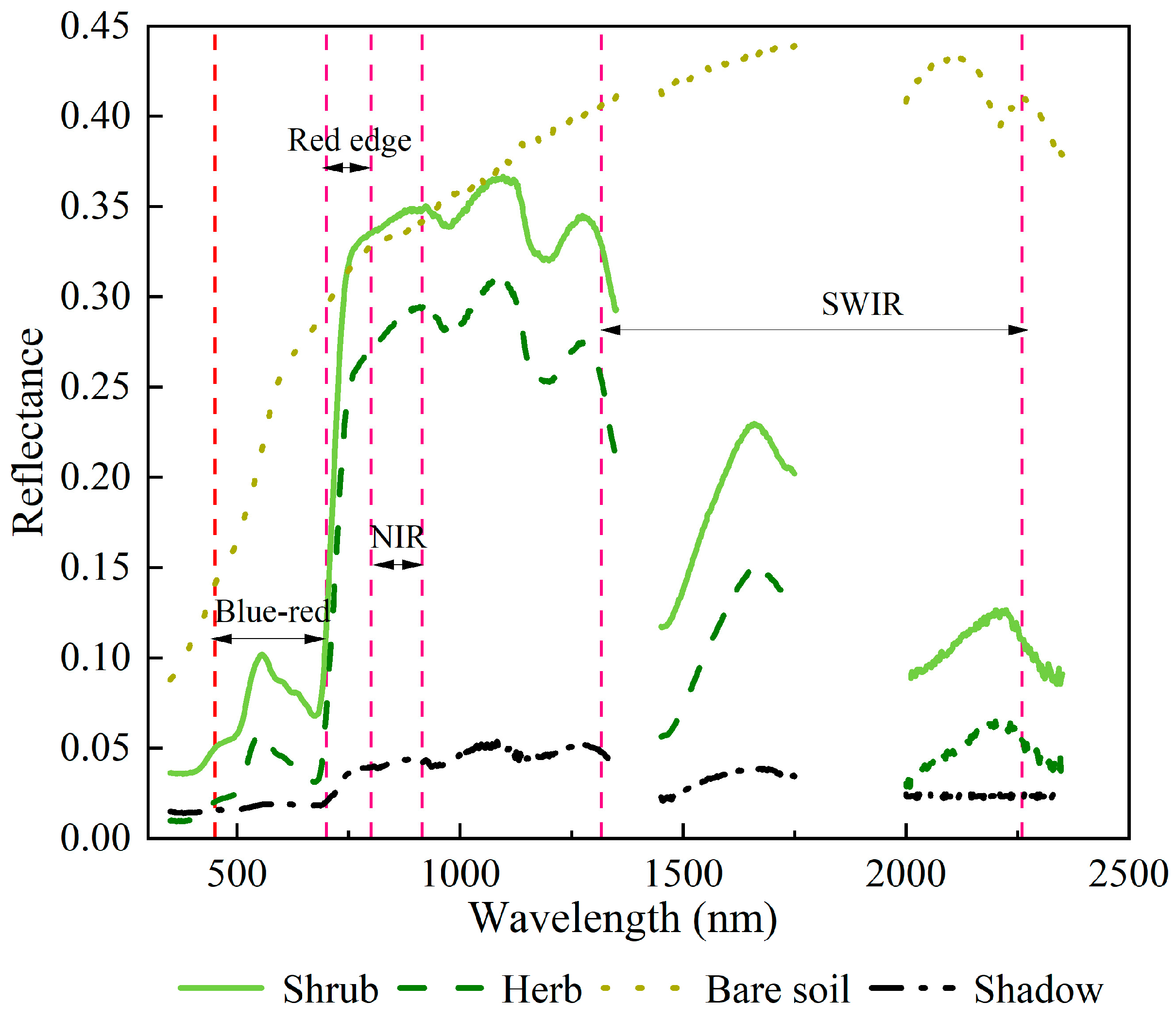
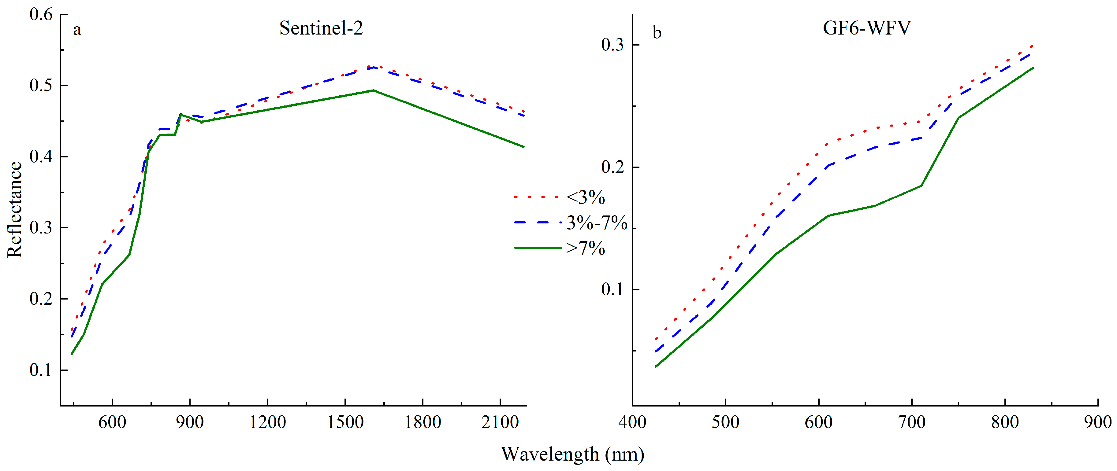
3.1. Spectral Feature Analysis

We acquired the spectra of shrubs, herbs, bare soil, and shadows in the study area through ground spectral observation. In order to eliminate the impact of changes in time and space on the spectra of various types of ground objects, five sets of spectral data were obtained for each type of ground object, i.e., shrubs, herbs, bare soil, and shadows, and the average value was considered the final spectrum. At the same time, the bands that were severely affected by the atmosphere and water vapor absorption bands were removed, while retaining spectral ranges of 350–1350 nm, 1450–1750 nm, and 2000–2350 nm [60]. The spectral curves are shown in Figure 3.

In Figure 3, it can be seen that the spectral curves of bare soil, vegetation, and shadow significantly differ, making it easier to distinguish between them. Due to the highly reflective nature of sandy land, the reflectance of bare soil is significantly higher than that of vegetation and shadows. Shadows have relatively low reflectivity throughout the entire wavelength range, with little fluctuation, and thus, they present significant differences in their spectral characteristics as compared to other types of ground objects. Both shrubs and herbs belong to vegetation, and their spectral curves have obvious wave crest and trough characteristics. Their waveforms are relatively similar; in the red edge band, the reflectivity of shrubs and herbs is almost the same, but in the band range of 350–700 nm and above 800 nm, the reflectivity of shrubs is slightly higher than that of grass, which has differences, making it possible to use a spectral mixture model to distinguish the two.

At the same time, to explore the differences in spectral characteristics of shrubs under different vegetation coverage, the spectral reflectance of Sentinel-2 and GF6-WFV corresponding to each interval was obtained according to the intervals indicated in Section 2.2.1. The results are presented in Figure 4.

With an increase in shrub vegetation coverage (Figure 4), absorption by the Caragana microphylia shrub community gradually increased in the green and red bands, and the slope of the red edge band (i.e., the first-order derivative value of the reflectance curve corresponding to the red edge position) gradually increased. The research area was in an arid and semi-arid region with sparse vegetation coverage. Regardless of the images being obtained from Sentinel-2 or GF6-WFV, the spectral curves of shrub vegetation under various coverage levels were relatively smooth (without obvious peaks or valleys). However, with an increase in shrub coverage, the volatility of the spectral curves of shrubs with coverage levels >7% increased as compared to the coverage range of 0–7%.

3.2. Estimation of Shrub Coverage for Linear Spectral Unmixing

Based on the spectral differences noted among bare soil, shadow, herbaceous vegetation, and shrub vegetation, the endmember spectra shown in Section 3.1 were resampled to the spectral ranges corresponding to Sentinel-2 and GF6-WFV. The FCLS algorithm was used for linear spectral unmixing of four endmembers, and the estimated shrub coverage is shown in

Table 4. Estimation of shrub coverage using Sentinel-2 and GF6-WFV.

Data	Method	R2	RMSE
Sentinel-2	FCLS	0.23	0.13
GF6-WFV		0.09	0.18

.

Table 4 indicates that when shrub coverage was estimated using GF6-WFV image data, R² was 0.09 and RMSE was 0.18; when it was estimated using Sentinel-2 image data, R² was 0.23 and RMSE was 0.13, showing a slight improvement in the accuracy as compared to the GF6-WFV image data. Overall, the estimation results of both methods were not good. Therefore, using mixed spectral unmixing to estimate shrub coverage in SEGs with medium-resolution multispectral images is not ideal. At the same time, to explore the ability to use the mixed spectral model to estimate shrub coverage under different shrub coverage levels in SEGs, this paper further analyzed shrub coverage estimation effects of the spectral mixture model under different shrub coverage levels, and the results are summarized in

Table 5. Estimation of different shrub cover categories using Sentinel-2 and GF6-WFV images.

Remote Sensing Image	Measured Shrub Coverage	Description	R2	RMSE
Sentinel-2	<3%	Shrubs and herbs cannot be distinguished	-	-
	3~7%	1/2 of the shrub coverage was successfully estimated	0.01	0.11
	>7%	4/5 the shrub coverage was successfully estimated	0.13	0.16
GF6-WFV	<3%	Shrubs and herbs cannot be distinguished	-	-
	3~7%	1/3 of the shrub coverage was successfully estimated	0.01	0.19
	>7%	1/2 of the shrub coverage was successfully estimated	0.02	0.22

.

For Sentinel-2 (Table 5), when the shrub coverage was less than 3%, the spectral mixing model did not recognize the shrub due to the low shrub coverage. When the shrub coverage ranges from 3% to 7%, half of the shrub coverage was successfully estimated. When the shrub coverage was above 7%, 4/5 of the shrub coverage was successfully estimated, and the estimation accuracy was greatly improved when the shrub coverage was greater than 7%. For GF6-WFV images, when the shrub coverage was less than 3%, the spectral mixing model could not recognize the shrubs as well. When the shrub coverage was between 3% to 7%, 1/3 of the shrub coverage was successfully estimated. When the shrub coverage was above 7%, 1/2 of the shrub coverage was successfully estimated. To sum up, shrub coverage affected the estimation accuracy of the LSMM to a certain extent. With an increase in shrub coverage, the probability of the LSMM identifying the shrubs increased, and the shrubs and herbs also showed an obvious lack of differentiation.

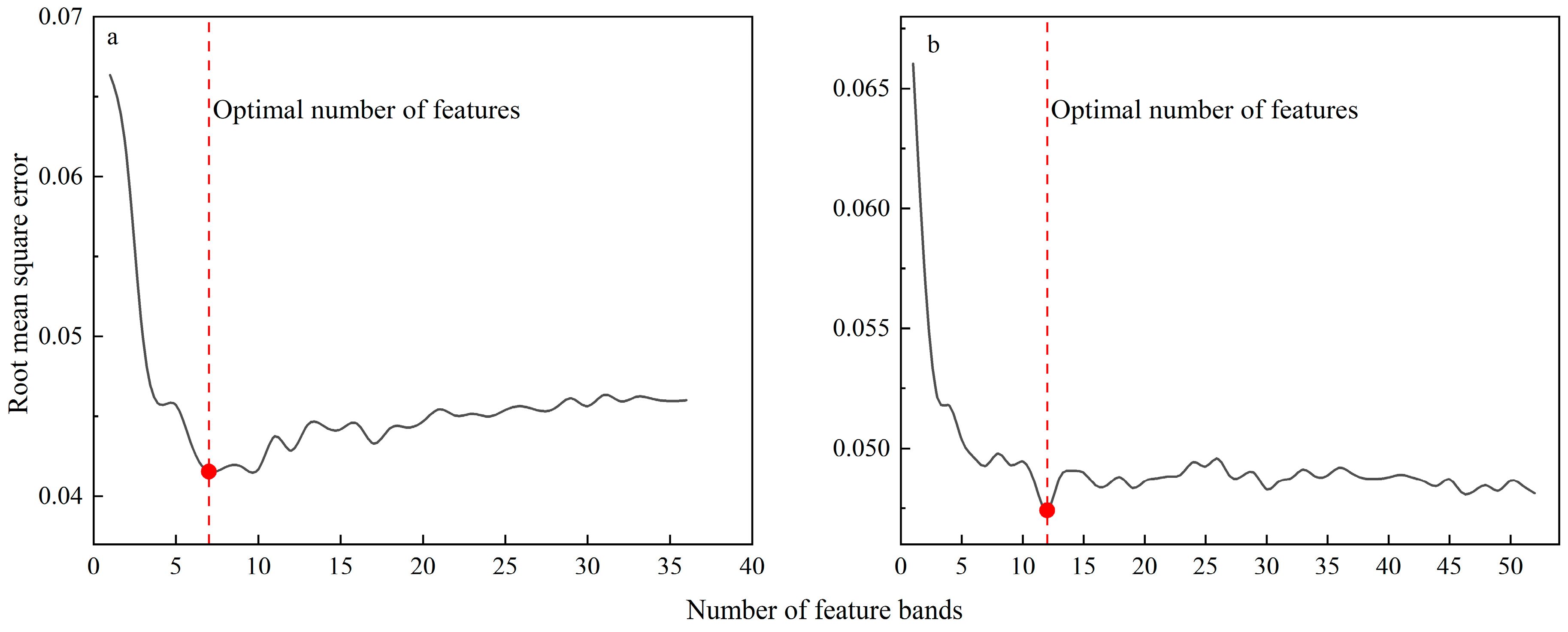
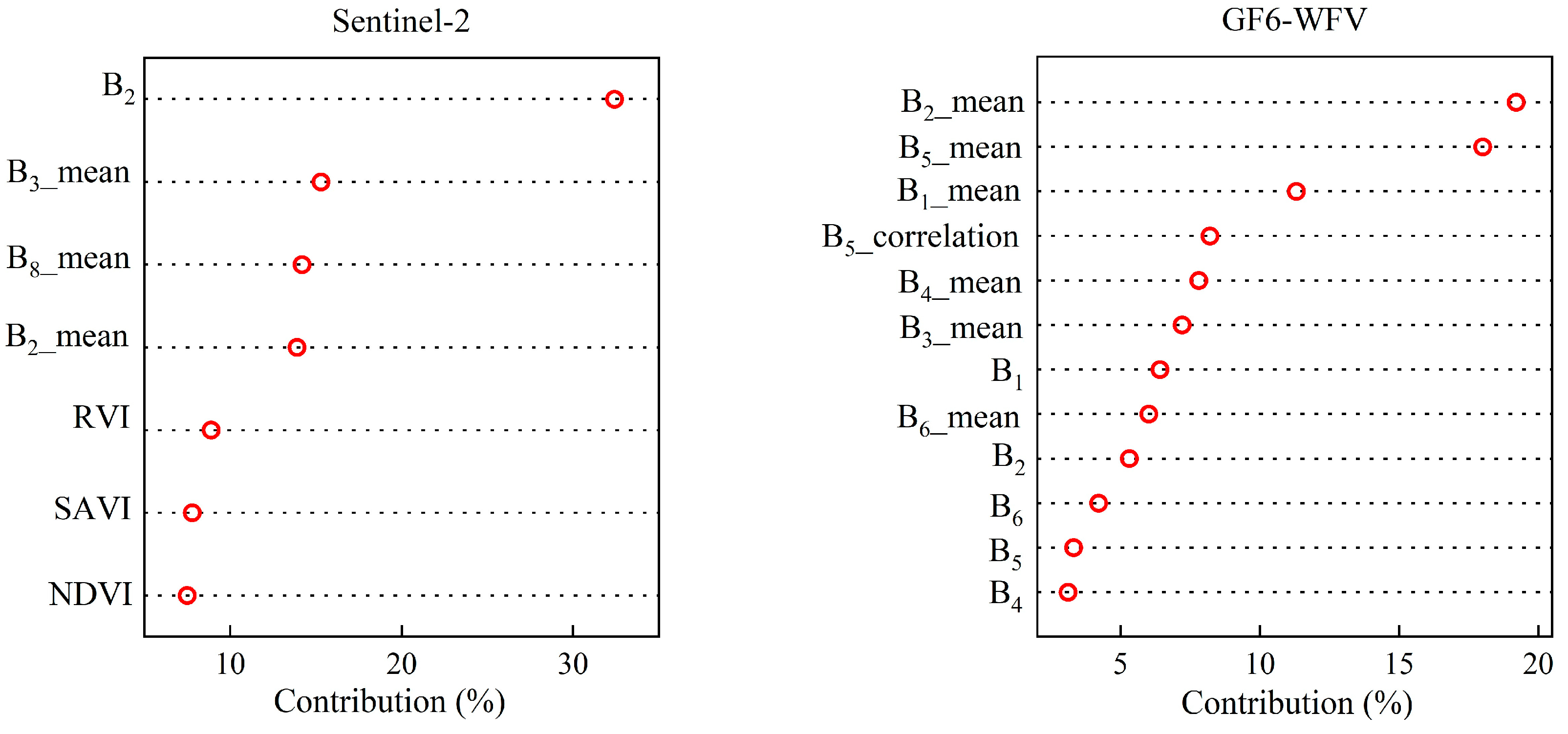
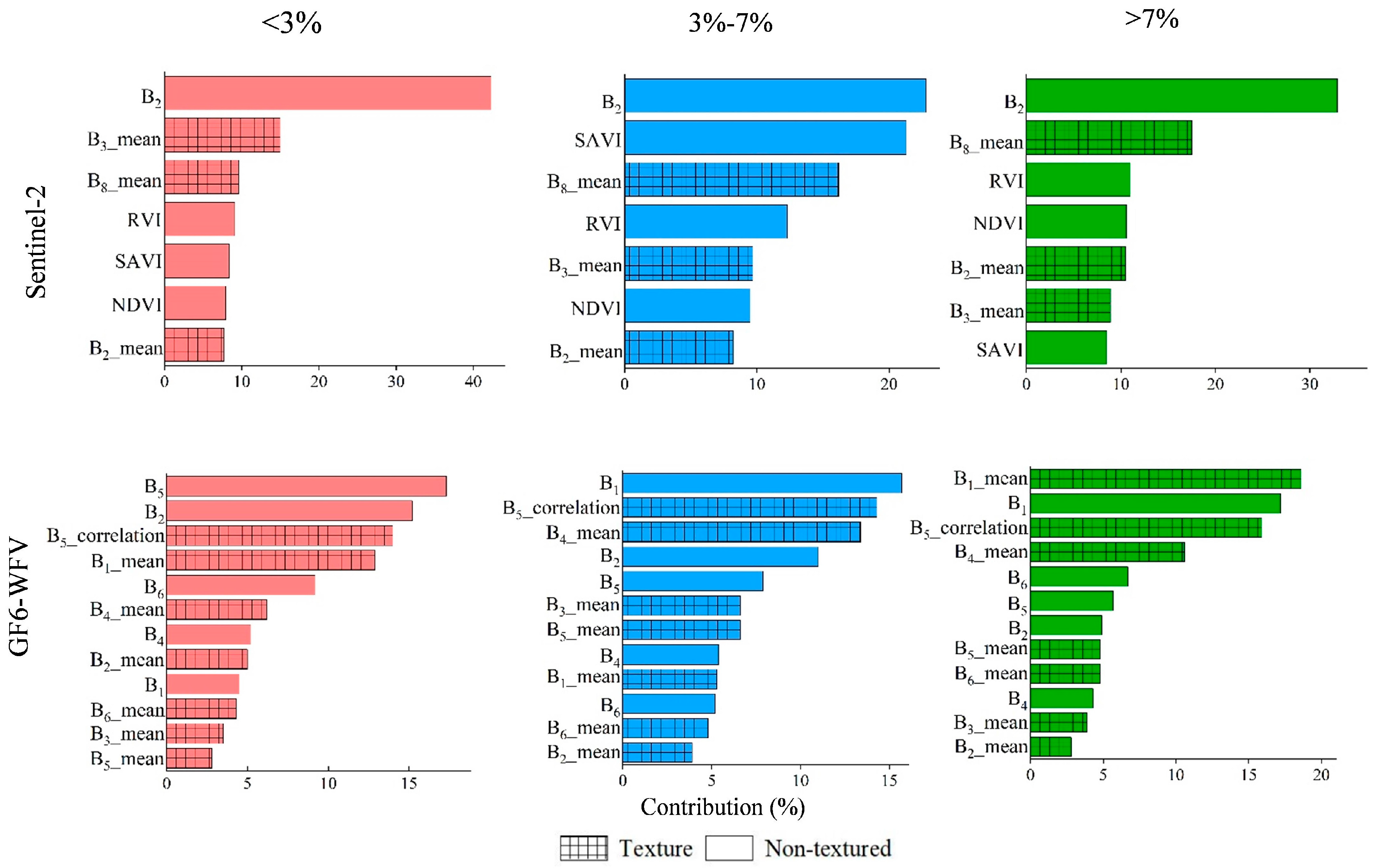
3.3. Remote Sensing-Based Selection of Feature Variables

The feature variables extracted from Sentinel-2 and GF6-WFV images were selected using RFE 5-fold cross-validation; results are shown in Figure 5.

As per Figure 5, as the number of features increases, RMSE first decreases and then increases; contrarily, increasing the number of features increases the complexity of the model. Therefore, it was necessary to optimize feature variables, while ensuring model accuracy. For the Sentinel-2 image data, seven feature variables were selected, namely SAVI and B₂_mean, B₂, B₈_mean, NDVI, RVI, and B₃_mean; i.e., the features were reduced by 80.6% as compared to the original number of features. For the GF6-WFV images, 12 feature variables were selected, namely B₁_mean, B₂_mean, B₃_mean, B₅_mean, B₆_mean, B₄_mean, B₁, B₆, B₅, B₄, B₂, and B₅_correlation. Here, features were reduced by 76.9% as compared to the original number of features.

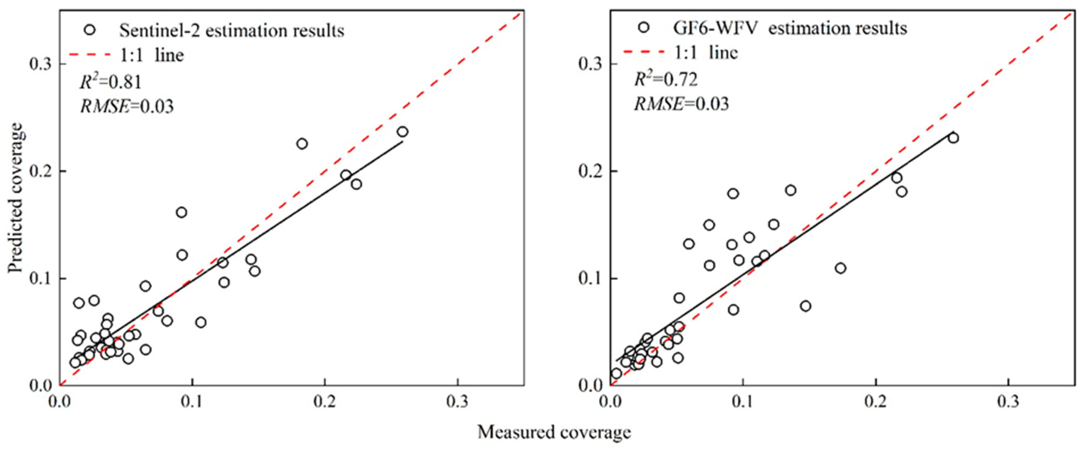
3.4. Estimation of Shrub Coverage Using the RF Model

Characteristic variables selected via Sentinel-2 and GF6-WFV were used to build the estimation model of RF shrub coverage as shown in Figure 6.

It can be seen from Figure 6 that when the Sentinel-2 image data were used to build the random forest-based estimation model for shrub coverage, the R² was 0.81 and RMSE was 0.03. When the GF6-WFV image data were used to build the random forest-based shrub coverage estimation model, the R² was 0.72 and the RMSE was 0.03. Overall, both the approaches achieved good estimation accuracy, but the estimation accuracy with the Sentinel-2 image was higher than that with the GF6-WFV image data. The method of building a random forest-based regression model to estimate shrub coverage with medium-resolution multispectral images was feasible, as it achieved higher estimation accuracy, provided improved spatial resolution of images, and enhanced model accuracy. The importance ranking of each variable involved in the estimation of the RF model is shown in Figure 7.

From Figure 7, it can be seen that for Sentinel-2 images, the blue band (B₂) was the most important with a contribution of 32.4%, followed by the green band textural mean feature (B₃_mean) with a contribution of 15.3%. Among the seven feature variables, three were accounted for by the textural features, with a total contribution of 43.4%. For GF6-WFV images, the green band textural mean (B₂_mean) had the highest importance with a contribution of 19.2%, followed by the red edge 1 band textural mean (B₅_mean) with a contribution of 18%. Among the 12 feature variables, textural features account for 7; the top-ranked feature contribution was by the textural features, accounting for a total of 77.7%. At the same time, it was found in Section 3.2 of this paper that the magnitude of the shrub coverage affected the estimation accuracy of the LSMM to a certain extent. Therefore, this paper further discusses the ability to use the RF model to estimate shrub coverage in different shrub coverage intervals. The results are shown in

Table 6. Results of the estimation of random forest under different shrub coverage.

Measured Shrub Coverage	Sentinel-2		GF6-WFV
	R2	RMSE	R2	RMSE
<3%	0.66	0.004	0.61	0.003
3~7%	0.53	0.005	0.45	0.007
>7%	0.67	0.039	0.66	0.040

and Figure 8.

As per Table 6, for the Sentinel-2 image data, the model exhibits good estimation accuracy, with an R² of 0.66, when in a low shrub coverage area (<3%). In a moderate shrub coverage area (3–7%), the R² decreased and the RMSE value improved. For a high shrub coverage area (>7%), the model reaches the highest R² of 0.67. For the GF6-WFV image data, the estimation accuracy of the model in areas with moderate shrub coverage was also poor. Additionally, the estimation accuracy of the model in areas with high shrub coverage was also higher than that in areas with low shrub coverage. In summary, both the Sentinel-2 and GF6-WFV images exhibit a common phenomenon, which is that their estimation models are more accurate in areas with low and high shrub coverage. However, in areas with moderate shrub coverage, their model accuracies are not as good; bushes in areas with medium coverage lower the accuracy of estimating the overall shrub coverage.

The importance ranking of each variable also varies under different coverage levels (Figure 8). For the Sentinel-2 images, the importance of the blue band (B₂) was highest in areas with high coverage, medium coverage, and low coverage. For the GF6-WFV images, in addition to low coverage areas, the importance of the blue band (B1) was also at a relatively high level in both medium and high coverage areas. It can be seen that the blue band made a significant contribution toward explaining the changes in shrub coverage, and thus, it has a potential for application in estimating shrub coverage. The contributions of textural features vary under different levels of shrub coverage. When in areas with low coverage, the textural proportions in the Sentinel-2 and GF6-WFV images were 32.3% and 48.7%, respectively. When in areas with medium coverage, the textural proportions under the Sentinel-2 and GF6-WFV images were 34.1% and 54.9%, respectively. When in areas with high coverage, the textural proportions under the Sentinel-2 and GF6-WFV images were 36.9% and 61.4%, respectively. As the shrub coverage increases, the shrub plane features will also be obvious; therefore, the influence of textural features on shrub coverage also significantly increases. The red edge band of the GF6-WFV images is rich in information. With the increase in shrub coverage, information on the red edge and red edge texture also contribute to better-explaining shrub coverage.

4. Discussion

4.1. Comparison between Ground-Measured and Aerial-Photo-Derived Shrub Coverage

The training and validation for spectral mixing models and random forest models in this study were supported by aerial photographs. The traditional way to obtain shrub coverage mainly depended on artificial ground acquisition, such as the sample line needling method, which selects a central position in each sample plot, uses RTK to obtain the center coordinates, starts from due north, and arranges three 30 m long sample lines at 60 degrees intervals. On the laid sample lines, the standard is to cover the ground with the flower pole vertically placed and touched, record the types of ground objects touched on the sampling line every 0.5 m (if the vegetation coverage is uniform, the interval distance can be appropriately increased), and the final shrub coverage is the ratio of the number of vegetation touched to the total number of samples sampled [27]. However, when this method is applied for investigating sparse and uneven shrub distribution in sample plots, the number of spline lines is prone to errors, difficult to control, and difficult to accurately represent the true situation of the overall sample plot. Drones are widely used in ecological monitoring due to their low cost, high flexibility, and ease of operation [61]. In this study, aerial photographs were used to calculate the shrub coverage of the sample plot. At first, the vegetation index was calculated through aerial photographs, and then the sample plots were divided on the aerial photographs to determine the threshold for distinguishing between shrubs and herbs. Finally, the number of shrub pixels within the sample plots was counted. From Figure 3, it can be seen that there is a significant spectral difference between herbaceous vegetation and shrub vegetation canopy within the visible light range. Therefore, threshold values can be well determined on high-resolution aerial photographs to distinguish shrubs and herbaceous vegetation. Fu et al. [62] calculated the vegetation index in the visible light band based on drone images and analyzed the reliability of using threshold values to estimate vegetation coverage. The results showed that the vegetation index threshold in the visible light band is highly sensitive to desert grasslands and can achieve high accuracy in vegetation coverage estimation. Nevertheless, variations in shooting time and weather conditions among different aerial photographs result in distinct thresholds.

4.2. Factors Influencing the Estimation of Shrub Coverage via LSMM and Comparison of Estimation Accuracy of the Different Remote Sensing Images

When using the LSMM to estimate shrub coverage in this paper, the estimation accuracy of Sentinel-2 was higher than that of GF6-WFV. The main reason may be that Sentinel-2 has more bands and can distinguish shrubs and herbs from more bands; Sentinel-2 also has a higher spatial resolution, and the degree of spectral mixing in each pixel is relatively low. It is easier to obtain endmember abundance using the LSMM. Ji et al. [45] used a linear spectral mixing model to perform three endmembers spectral unmixing on images with different spatial resolutions. The main images used were Landsat8-OLI (spatial resolution 30 m), GF1-WFV (spatial resolution 16 m), and Sentinel-2 (spatial resolution 10 m). The R² values were 0.39, 0.54, and 0.71, respectively. The improvement in image spatial resolution contributed to the estimation accuracy of spectral mixing models [63]. The Sentinel-2 sensor with a narrower band has better performance in estimating vegetation coverage than GF6-WFV, as the narrow band is more sensitive to changes in vegetation characteristics and can reduce the impact of soil background on sparse vegetation coverage areas [64].

In this study, the accuracy of shrub coverage estimation with the spectral mixture model was low. Contrarily, Chen et al. [65] estimated vegetation coverage with the pixel dichotomy model and the spectral mixture model based on Landsat8 OLI image; the research has shown that the spectral mixture model has higher accuracy, and the accuracy of vegetation coverage extraction was 85.31%, mainly because the mixed spectrum that was to be decomposed belonged to vegetation and bare soil of different ground object types. This study aimed to estimate the coverage of shrubs in SEGs, and the mixed spectra that were to be decomposed comprised shrubs and herbs of the same genus of vegetation. The research results of Asner [66] and Smith [67] also indicated that community structure and species composition are important factors that affect the unmixing of mixed spectra. At the same time, due to the limitations of the field surveys, the measured canopy spectrum could exhaust the spatial heterogeneity of herbaceous and shrub vegetation in the study area [18], which may be another reason for the poor estimation quality using the LSMM.

4.3. Factors Influencing the Estimation of Shrub Coverage with the RF Model and Comparison of Estimation Accuracy of the Different Remote Sensing-Based Imaging

This study successfully estimated shrub coverage in SEGs through the RF model and achieved good estimation accuracy. By comparing its modeling feature factors, it can be found that whether it is Sentinel-2 images or GF6-WFV images, the total contribution of texture features has a certain impact on the model. This was mainly because there were differences in the structure and growth morphology between shrub and herbaceous vegetation, leading to significant differences in the texture reflected by the remote sensing images of these two vegetation types. Therefore, textural features as the preferred feature variables can help establish a model for estimating shrub coverage in SEGs and improve the accuracy of model estimation. This is consistent with the research results of Zhang et al. [35]. The phenomenon, like the model, did not show improved performance as the increase in shrub coverage, which is shown in Table 6, may result from the different infrared wave scattering mechanisms with different land cover. Previous research demonstrated that the scattering from soil and vegetation are mixed and are difficult to be separated when the vegetation coverage is moderate. Due to the similar scattering proportion of shrubs and herbs, the difference between them is no longer significant and lead to increased difficulty in extracting shrub coverage [51]. However, for vegetation with high and low coverage, due to lack of sufficient soil information in the former and insufficient vegetation to transmit canopy scattering and soil reflection information in the latter, the information received by the sensor is relatively less affected by the soil background [68], and there is a significant spectral difference between shrubs and herbs in this range, which is conducive to the extraction of shrub coverage.

The blue band visible in Figure 8 significantly contributes to the estimation of shrub coverage at different levels of shrub coverage. Studies have shown that chlorophyll is more sensitive to the blue band, and thus strongly absorbs in its range [69]. However, in this study, the canopy of shrub vegetation in the study area was darker in color and contains more chlorophyll than that of herbaceous vegetation. Eventually, the blue band became more sensitive to the coverage of shrubs. Compared with the spectral mixture model, regardless of it being based on image features from Sentinel-2 or GF6-WFV, the estimation accuracy of the RF model was higher. At the same time, with this estimation model, the estimation accuracy of Sentinel-2 was also higher than that of GF6-WFV. Therefore, in the SEG, the RF model was more suitable to estimate shrub coverage, which can also effectively improve the estimation accuracy of shrub coverage in large areas.

4.4. Limitations and Future Research Directions

When using the spectral mixture model to estimate shrub coverage in SEGs, the differentiation between shrub and herb is insufficient. In future research, attempts are needed to obtain hyperspectral data, such as the ZY-1 02D [70,71,72], to distinguish shrubs and herbs using a greater number of bands and improve the accuracy of shrub coverage estimation. Some studies show that the withering and yellowing period of the Caragana microphylla shrub in the study area differs from that of the herbaceous vegetation. The Caragana microphylla shrub withers and yellows in early October, and the herbaceous vegetation withers and yellows in early September [18]. The next steps of research can utilize the differences in vegetation phenological characteristics during this period to establish a shrub coverage estimation model, which may show better results. In addition, shrub coverage is also affected by factors, such as precipitation, soil, and shape [73]. In the future, variables, such as precipitation, soil, and shape, can be considered for the construction of the model, which may help to optimize the existing RF model.

5. Conclusions

This study considers the SEG in Xilingol as the study area and extracts the characteristic factors based on imaging data from remote sensing with Sentinel-2 and GF6-WFV. By discussing the spectral differences between herbaceous vegetation and shrub vegetation, a spectral mixture model and an RF model were constructed; their estimation accuracies were compared and analyzed. The main conclusions were as follows:

(1)

In the SEG, using the LSMM, estimation of shrub coverage could be achieved with medium-resolution images. Compared with the RF model, its estimation effect can still be improved; furthermore, it shows an obvious lack of differentiation between shrubs and herbs. In addition, the shrub coverage affects the estimation accuracy of the LSMM to a certain extent.

(2)

The RF model showed high estimation accuracy when estimating shrub coverage in the SEG using Sentinel-2 imaging, with an estimation accuracy, R², of 0.81 and an RMSE of 0.03. The estimation accuracy, R², of the GF6-WFV image is 0.72 and RMSE is 0.03. Especially for estimation models with high shrub coverage, the model accuracy reaches the highest level.

(3)

In the Sentinel-2 images, the contribution of texture features is 43.4%; in the GF6-WFV images, the contribution of texture features is 77.7%. Therefore, texture features as the preferred feature variables can help to construct a model for estimating shrub coverage in SEG and improve the estimation accuracy of the model.

(4)

Whether in the LSMM or in the RF model, the Sentinel-2 image may provide better estimation than the GF6-WFV imaging; these data have great potential to monitor SEGs.

References

1. Feng, H.; Zou, B.; Luo, J. Coverage-Dependent Amplifiers of Vegetation Change on Global Water Cycle Dynamics. J. Hydrol. 2017, 550, 220–229. [Google Scholar] [CrossRef]
2. Feng, L.L.; Jia, Z.Q.; Li, Q.X.; Zhao, A.Z.; Zhao, Y.L.; Zhang, Z.J. Spatiotemporal Change of Sparse Vegetation Coverage in Northern China. J. Indian Soc. Remote Sens. 2019, 47, 18–26. [Google Scholar] [CrossRef]
3. Chen, L.Y.; Shen, H.H.; Fang, J.Y. Shrub Encroached Grassland: A New Vegetation Type. Chin. J. Nat. 2014, 36, 391–396. [Google Scholar]
4. Archer, S.; Scifres, C.; Bassham, C.R.; Maggio, R. Autogenic Succession in a Subtropical Savanna: Conversion of Grassland to Thorn Woodland. Ecol. Monogr. 1988, 58, 111–127. [Google Scholar] [CrossRef]
5. Cai, Y.R.; Yan, Y.C.; Wang, C.; Xu, D.W.; Wang, X.; Xin, X.P.; Chen, J.Q.; Eldridge, D.J. Effect of Shrubs on Soil Saturated Hydraulic Conductivity Depends on the Grazing Regime in a Semi-Arid Shrub-Encroached Grassland. Catena 2021, 207, 105680. [Google Scholar] [CrossRef]
6. Zhao, Y.J.; Liu, X.L.; Wang, Y.; Zheng, Z.J.; Zheng, S.X.; Zhao, D.; Bai, Y.F. UAV-Based Individual Shrub Aboveground Biomass Estimation Calibrated against Terrestrial LiDAR in a Shrub-Encroached Grassland. Int. J. Appl. Earth Obs. Geoinf. 2021, 101, 102358. [Google Scholar] [CrossRef]
7. Peng, H.Y.; Li, X.Y.; Tong, S.Y. Advance in Shrub Encroachment in Arid and Semiarid Region. Acta Pratacult. Sin. 2014, 23, 313–322. [Google Scholar]
8. Jurena, P.-N.; Archer, S. Woody Plant Establishment and Spatial Heterogeneity in Grasslands. Ecology 2003, 84, 907–919. [Google Scholar] [CrossRef]
9. Wang, Q.; Xie, Y.F. Methods of Turf Quality Evaluation. Pratacult. Sci. 1993, 10, 69–73. [Google Scholar]
10. Zhang, Y.R.; Liu, T.X.; Tong, X.; Duan, L.M.; Jia, T.Y.; Ji, Y.X. Inversion of Vegetation Coverage Based on Multi-Source Remote Sensing Data and Machine Learning Method in Horqin Sandy Land, China. J. Desert Res. 2022, 42, 187–195. [Google Scholar]
11. Du, M.M.; Li, M.Z.; Noguchi, N.; Ji, J.T.; Ye, M.C. Retrieval of Fractional Vegetation Cover from Remote Sensing Image of Unmanned Aerial Vehicle Based on Mixed Pixel Decomposition Method. Drones 2023, 7, 43. [Google Scholar] [CrossRef]
12. Hu, J.Y.; Yue, J.B.; Xu, X.; Han, S.Y.; Sun, T.; Liu, Y.; Feng, H.K.; Qiao, H.B. UAV-Based Remote Sensing for Soybean FVC, LCC, and Maturity Monitoring. Agriculture 2023, 13, 692. [Google Scholar] [CrossRef]
13. Meng, B.; Gao, J.; Liang, T.; Cui, X.; Ge, J.; Yin, J.; Feng, Q.; Xie, H. Modeling of Alpine Grassland Cover Based on Unmanned Aerial Vehicle Technology and Multi-Factor Methods: A Case Study in the East of Tibetan Plateau, China. Remote Sens. 2018, 10, 320. [Google Scholar] [CrossRef]
14. Kattenborn, T.; Lopatin, J.; Förster, M.; Andreas, C.B.; Fabian, E.F. UAV Data as Alternative to Field Sampling to Map Woody Invasive Species Based on Combined Sentinel-1 and Sentinel-2 Data. Remote Sens. Environ. 2019, 227, 61–73. [Google Scholar] [CrossRef]
15. Liu, Y.H.; Cai, Z.L.; Bao, N.S.; Liu, S.J. Research of Grassland Vegetation Coverage and Biomass Estimation Method Based on Major Quadrat from UAV Photogrammetry. Ecol. Environ. 2018, 27, 2023–2032. [Google Scholar]
16. Cao, C.X.; Chen, W.; Li, G.H.; Jia, H.C.; Ji, W.; Xu, M.; Gao, M.X.; Ni, X.L.; Zhao, J.; Zheng, S.; et al. The Retrieval of Shrub Fractional Cover Based on a Geometric-Optical Model in Combination with Linear Spectral Mixture Analysis. Remote Sens. 2011, 37, 348–358. [Google Scholar] [CrossRef]
17. Yang, F.; Li, J.L.; Yang, W.Y.; Qian, Y.R.; Yang, Q.; Du, Z.Q. Assessing Vegetation Coverage of Desert Grassland Based on Linear Spectral Mixture Mode. Trans. Chin. Soc. Agric. Eng. 2012, 28, 243–247. [Google Scholar]
18. Liu, T.Y.; Zhao, X.; Shen, H.H.; Hu, H.F.; Huang, W.J.; Fang, J.Y. Spectral Feature Differences between Shrub and Grass Communities and Shrub Coverage Retrieval in Shrub-Encroached Grassland in Xianghuang Banner, Nei Mongol, China. Chin. J. Plant Ecol. 2016, 40, 969–979. [Google Scholar]
19. Gao, L.; Wang, X.F.; Johnson, B.A.; Tian, Q.J.; Wang, Y.; Verrelst, J.; Mu, X.H.; Gu, X.F. Remote Sensing Algorithms for Estimation of Fractional Vegetation Cover Using Pure Vegetation Index Values: A Review. ISPRS J. Photogramm. Remote Sens. 2020, 159, 364–377. [Google Scholar] [CrossRef]
20. Li, L.Y.; Mu, X.H.; Jiang, H.L.; Chianucci, F.; Hu, R.H.; Song, W.J.; Qi, J.B.; Liu, S.Y.; Zhou, J.X.; Chen, L.; et al. Review of Ground and Aerial Methods for Vegetation Cover Fraction (fCover) and Related Quantities Estimation: Definitions, Advances, Challenges, and Future Perspectives. ISPRS J. Photogramm. Remote Sens. 2023, 199, 133–156. [Google Scholar] [CrossRef]
21. Yang, J.; Shi, M.C.; Yang, J.Y. Vegetation Coverage Inversion Based on Combined Active and Passive Remote Sensing: A Case Study of the Baiyangdian-Daqinghe Basin. J. Resour. Ecol. 2023, 14, 591–603. [Google Scholar]
22. Ge, J.; Meng, B.P.; Liang, T.G. Modeling Alpine Grassland Cover Based on MODIS Data and Support Vector Machine Regression in the Headwater Region of the Huanghe River, China. Remote Sens. Environ. 2018, 218, 162–173. [Google Scholar] [CrossRef]
23. Andrés, E.; Alejandro, U.; María, G.A.; González, E.M. Monitoring Rainfed Alfalfa Growth in Semiarid Agrosystems Using Sentinel-2 Imagery. Remote Sens. 2021, 13, 4719. [Google Scholar]
24. Hu, Q.; Yang, J.Y.; Xu, B.D.; Huang, J.X.; Muhammad, S.M.; Yin, G.F.; Zeng, Y.L.; Zhao, J.; Liu, K. Evaluation of Global Decametric-Resolution LAI, FAPAR and FVC Estimates Derived from Sentinel-2 Imagery. Remote Sens. 2020, 12, 912. [Google Scholar] [CrossRef]
25. Wang, Y.F.; Tan, L.; Wang, G.Y.; Sun, X.Y.; Xu, Y.N. Study on the Impact of Spatial Resolution on Fractional Vegetation Cover Extraction with Single-Scene and Time-Series Remote Sensing Data. Remote Sens. 2022, 14, 4165. [Google Scholar] [CrossRef]
26. Zhao, H.F.; Lu, Z.; Yi, Y.; Zhao, J.Z.; Wang, D.Q.; Shi, Y.; Chen, Y. Research on Remote Sensing Estimation of Vegetation Coverage Based on Gaofen-6 Satellite. Geomat. Spat. Inf. Technol. 2022, 45, 19–23. [Google Scholar]
27. Shao, J. Monitoring of Shrub Encroachment into Grassland by Utilizing Sentinel-1 and Sentinel-2 Jointly; University of Chinese Academy of Sciences: Beijing, China, 2020. [Google Scholar]
28. Wu, R.H.; Zhang, X.H.; Chang, S.; Yu, H.B.; Li, X.; Zhang, Q.F. Spatial Differentiation Characteristics of Soil Organic Carbon, Total Nitrogen and Total Phosphorus in Xilingol Steppe. North. Hortic. 2023, 70–79. [Google Scholar]
29. Zhou, Y.; Chen, J.; Chen, X.H.; Cao, X.; Zhu, X.L. Two Important Indicators with Potential to Identify Caragana Microphylla in Xilin Gol Grassland from Temporal MODIS Data. Ecol. Indic. 2013, 34, 520–527. [Google Scholar] [CrossRef]
30. Wu, N.; Crusiol, L.G.T.; Liu, G.X.; Wuyun, D.; Han, G. Comparing Machine Learning Algorithms for Pixel/Object-Based Classifications of Semi-Arid Grassland in Northern China Using Multisource Medium Resolution Imageries. Remote Sens. 2023, 15, 750. [Google Scholar] [CrossRef]
31. Ji, C.C.; Jia, Y.H.; Li, X.S.; Wang, J.Y. Research on Linear and Nonlinear Spectral Mixture Models for Estimating Vegetation Fractional Cover of Nitraria Bushes. J. Remote Sens. 2016, 20, 1402–1412. [Google Scholar]
32. Lu, H.; Fan, T.X.; Ghimire, P.; Deng, L. Experimental Evaluation and Consistency Comparison of UAV Multispectral Minisensors. Remote Sens. 2020, 12, 2542. [Google Scholar] [CrossRef]
33. Maulit, A.; Nugumanova, A.; Apayev, K.; Baiburin, Y.; Sutula, M. A Multispectral UAV Imagery Dataset of Wheat, Soybean and Barley Crops in East Kazakhstan. Data 2023, 8, 88. [Google Scholar] [CrossRef]
34. Brunier, G.; Oiry, S.; Gruet, Y.; Dubois, S.F.; Barillé, L. Topographic Analysis of Intertidal Polychaete Reefs (Sabellaria alveolata) at a Very High Spatial Resolution. Remote Sens. 2022, 14, 307. [Google Scholar] [CrossRef]
35. Zhang, C.Q.; Sun, B.; Hong, L.; Gao, Z.H.; Wang, S.S. Identification of Shrub Encroachment in Grassland by Using Multi-Source Remote Sensing Data. Spacecr. Recover. Remote Sens. 2022, 43, 123–137. [Google Scholar]
36. Chen, L.Y.; Li, H.; Zhang, P.J.; Zhao, X.; Zhou, L.H.; Liu, T.Y.; Hu, H.F.; Bai, Y.F.; Shen, H.H.; Fang, J.Y. Climate and Native Grassland Vegetation as Drivers of the Community Structures of Shrub-Encroached Grasslands in Inner Mongolia, China. Landsc. Ecol. 2015, 30, 1627–1641. [Google Scholar] [CrossRef]
37. Maciej, A.; Mirosław, B.; Katarzyna, L.N.; Marta, N.; Tomasz, N. Impairing Land Registry: Social, Demographic, and Economic Determinants of Forest Classification Errors. Remote Sens. 2020, 12, 2628. [Google Scholar]
38. Xie, E.H.; Wu, J.E.; Yang, K. Mass Concentration in Inversion for Chlorophyll a Erhai Lake Based on Sentinel-2. Chin. J. Environ. Eng. 2022, 16, 3058–3069. [Google Scholar]
39. Wang, X.X.; Lu, X.P.; Meng, Q.Y.; Li, G.Q.; Wang, J.; Zhang, L.L.; Yang, Z.N. Inversion of Leaf Area Index Based on GF6-WFV Spectral Vegetation Index Model. Spectrosc. Spectr. Anal. 2022, 42, 2278–2283. [Google Scholar]
40. Li, Y.F.; Sun, B.; Gao, Z.H.; Su, W.S.; Wang, B.Y.; Yan, Z.Y.; Gao, T. Extraction of Rocky Desertification Information in Karst Area by Using Different Multispectral Sensor Data and Multiple Endmember Spectral Mixture Analysis Method. Front. Environ. Sci. 2022, 10, 2085. [Google Scholar] [CrossRef]
41. Gao, D.Y. Remote Sensing Monitoring of Dynamic Change of Vegetation Coverage in Reservoir Basin Based on Mixed Pixel Decomposition; Zhengzhou University: Zhengzhou, China, 2021. [Google Scholar]
42. Zhang, X.; Shang, K.; Chen, Y.; Xu, X. Estimating Ecological Indicators of Karst Rocky Desertification by Linear Spectral Unmixing Method. Int. J. Appl. Earth Obs. Geoinf. 2014, 31, 86–94. [Google Scholar] [CrossRef]
43. Heinz, D.C.; Chang, C.I. Fully Constrained Least Squares Linear Spectral Mixture Analysis Method for Material Quantification in Hyperspectral Imagery. IEEE Trans. Geosci. Remote Sens. 2001, 39, 529–545. [Google Scholar] [CrossRef]
44. Wang, L.G.; Liu, D.F.; Wang, Q.M. Geometric Method of Fully Constrained Least Squares Linear Spectral Mixture Analysis. IEEE Trans. Geosci. Remote Sens. 2013, 51, 3558–3566. [Google Scholar] [CrossRef]
45. Ji, C.C. Research on Muti-Scale Spectral Mixture Analysis Method for Sparse Photosynthetic/Non-Photosynthetic Vegetation in Arid Area; Wuhan University: Wuhan, China, 2018. [Google Scholar]
46. Haralick, R.M.; Shanmugam, K.; Dinstein, I. Textural Features for Image Classification. IEEE Trans. Syst. Man Cybern. 1973, 3, 610–621. [Google Scholar] [CrossRef]
47. Chen, Y.; Yang, F.Y. Analysis of Image Texture Features Based on Gray Level Co-Occurrence Matrix. Appl. Mech. Mater. 2012, 1975, 204–208. [Google Scholar] [CrossRef]
48. Liu, L.Y.; Fan, X.J. The Design of System to Texture Feature Analysis Based on Gray Level Co-Occurrence Matrix. Appl. Mech. Mater. 2015, 3759, 727–728. [Google Scholar] [CrossRef]
49. Broge, N.H.; Leblanc, E. Comparing Prediction Power and Stability of Broadband and Hyperspectral Vegetation Indices for Estimation of Green Leaf Area Index and Canopy Chlorophyll Density. Remote Sens. Environ. 2001, 76, 156–172. [Google Scholar] [CrossRef]
50. Jiang, Z.Y.; Huete, A.R.; Didan, K. Development of a Two-Band Enhanced Vegetation Index without a Blue Band. Remote Sens. Environ. 2008, 112, 3833–3845. [Google Scholar] [CrossRef]
51. Huete, A.R. A Soil-Adjusted Vegetation Index (SAVI). Remote Sens. Environ. 1988, 25, 295–309. [Google Scholar] [CrossRef]
52. Zhao, Y.S. Principles and Methods of Remote Sensing Application Analysis; Science Press: Beijing, China, 2003. [Google Scholar]
53. Jaber, J.; Anis, Z. Feature Selection Engineering for Credit Risk Assessment in Retail Banking. Information 2023, 14, 200. [Google Scholar]
54. Gao, H.Y.; Hou, M.J.; Ge, J.; Bao, X.Y.; Li, Y.C.; Liu, J.; Feng, Q.S.; Liang, T.G.; He, J.S.; Qian, D.W. Hyperspectral Estimation of Aboveground Biomass of Alpine Grassland Based on Random Forest. Acta Agrestia Sin. 2021, 29, 1757–1768. [Google Scholar]
55. Darst, B.F.; Malecki, K.C.; Engelman, C.D. Using Recursive Feature Elimination in Random Forest to Account for Correlated Variables in High Dimensional Data. BMC Genet. 2018, 19, 65. [Google Scholar] [CrossRef]
56. Ke, Y.; David, Z. Feature Selection and Analysis on Correlated Gas Sensor Data with Recursive Feature Elimination. Sens. Actuators B Chem. 2015, 212, 353–363. [Google Scholar]
57. Breiman, L. Random Forests. Mach. Learn. 2001, 45, 5–32. [Google Scholar] [CrossRef]
58. Belgiu, M.; Drăguţ, L. Random Forest in Remote Sensing: A Review of Applications and Future Directions. ISPRS J. Photogramm. Remote Sens. 2016, 114, 24–31. [Google Scholar] [CrossRef]
59. Rodriguez-Galiano, V.F.; Ghimire, B.; Rogan, J.; Chica-Olmo, M.; Rigol-Sanchez, J.P. An Assessment of the Effectiveness of a Random Forest Classifier for Land-Cover Classification. ISPRS J. Photogramm. Remote Sens. 2012, 67, 93–104. [Google Scholar] [CrossRef]
60. Zheng, G.X.; Li, X.S.; Zhang, K.X.; Wang, J.Y. Spectral Mixing Mechanism Analysis of Photosynthetic/Non-Photosynthetic Vegetation and Bared Soil Mixture in the Hunshandake Sandy Land. Spectrosc. Spectr. Anal. 2016, 36, 1063–1068. [Google Scholar]
61. Feng, J.L.; Liu, K.; Zhu, Y.H.; Li, Y.; Liu, L.; Meng, L. Application of Unmanned Aerial Vehicles to Mangrove Resources Monitoring. Trop. Geogr. 2015, 35, 35–42. [Google Scholar]
62. Fu, S.; Feng, Q.S.; Dang, J.Y.; Lei, K.X.; Qiao, W.X.; Liang, T.G.; Pan, D.R.; Sun, B.; Jiang, J.C. Comparison of Grassland Vegetation Coverage Extraction Algorithms from UAV Technology. Pratacult. Sci. 2022, 39, 455–464. [Google Scholar]
63. Gessner, U.; Machwitz, M.; Conrad, C.; Dech, S. Estimating the Fractional Cover of Growth Forms and Bare Surface in Savannas. A Muli-Resolution Approach Based on Regression Tree Ensembles. Remote Sens. Environ. 2013, 129, 90–102. [Google Scholar] [CrossRef]
64. Thenkabail, P.S.; Smith, P.B.; Pauw, E.D. Hyperspectral Vegetation Indices and Their Relationships with Agricultural Crop Characteristics. Remote Sens. Environ. 2000, 71, 158–182. [Google Scholar] [CrossRef]
65. Chen, H.B.; Huang, B.B.; Peng, D.L. Comparison of Pixel Decomposition Models for the Estimation of Fractional Vegetation Coverage. J. Northwest For. Univ. 2018, 33, 203–207. [Google Scholar]
66. Asner, G.P. Biophysical and Biochemical Sources of Variability in Canopy Reflectance. Remote Sens. Environ. 1998, 64, 234–253. [Google Scholar] [CrossRef]
67. Smith, M.O.; Ustin, S.L.; Adanms, J.B.; Gillespie, A.R. Vegetation in Deserts: I. A Regional Measure of Abundance from Multispectral Images. Remote Sens. Environ. 1990, 31, 1–26. [Google Scholar] [CrossRef]
68. Huete, A.R.; Jackson, R.D.; Post, D.F. Spectral Response of a Plant Canopy with Different Soil Backgrounds. Remote Sens. Environ. 1985, 17, 37–53. [Google Scholar] [CrossRef]
69. Xu, Y.F. Parameter Retrieval and Comprehensive Growth Monitoring of Winter Wheat Based on UAV Multispectral Remote Sensing; Anhui University of Science and Technology: Huainan, China, 2022. [Google Scholar]
70. Yang, Z.N.; Gong, C.L.; Ji, T.M.; Hu, Y.; Li, L. Water Quality Retrieval from ZY1-02D Hyperspectral Imagery in Urban Water Bodies and Comparison with Sentinel-2. Remote Sens. 2022, 14, 5029. [Google Scholar] [CrossRef]
71. Lu, H.; Qiao, D.Y.; Li, Y.X.; Wu, S.; Deng, L. Fusion of China ZY-1 02D Hyperspectral Data and Multispectral Data: Which Methods Should Be Used? Remote Sens. 2021, 13, 2354. [Google Scholar] [CrossRef]
72. Tan, W.; Wang, S.S.; He, H.Y.; Qi, W.W. Reconstructing Coastal Blue with Blue Spectrum Based on ZY-1(02D) Satellite. Optik 2021, 242, 166901. [Google Scholar] [CrossRef]
73. Lou, P.Q.; Lou, P.Q.; Chen, J.; Zhu, X.F.; Wu, X.D.; Li, R.; Xie, C.W.; HU, G.J. Solifluction Identification in the Qilian Mountains Based on High Resolution Remote Sensing Imagery and Ensemble Machine Learning. J. Glaciol. Geocryol. 2023, 45, 786–797. [Google Scholar]
Figure 1. (a) Location and sample distribution of the study area; (b) shrub-encroached grasslands (SEGs) captured on the ground; (c) SEGs captured via an unmanned aerial vehicle.
Remotesensing 15 05488 g001
Figure 2. Process for estimating shrub coverage.
Remotesensing 15 05488 g002
Figure 3. ASD FieldSpec Pro FR 2500: the spectra of each ground object. Note: NIR represents the near-infrared band, and SWIR represents the short-wave infrared band.
Remotesensing 15 05488 g003
Figure 4. Spectral curves of shrubs under different levels of vegetation cover. Note: (a) shows the spectral curves of shrubs obtained under different vegetation cover levels with Sentinel-2. (b) shows the spectral curves of shrubs obtained under different vegetation cover levels with GF6-WFV.
Remotesensing 15 05488 g004
Figure 5. Remote sensing image feature variable selection with (a) Sentinel-2; (b) GF6-WFV.
Remotesensing 15 05488 g005
Figure 6. Results of estimation and precision tests of shrub coverage with the random forest model.
Remotesensing 15 05488 g006
Figure 7. Distribution of variable importance in the random forest model.
Remotesensing 15 05488 g007
Figure 8. Importance ranking of variables under different levels of coverage.
Remotesensing 15 05488 g008