Evaluation of MAX-DOAS Profile Retrievals under Different Vertical Resolutions of Aerosol and NO₂ Profiles and Elevation Angles

Abstract

In the Multi-Axis Differential Absorption Spectroscopy (MAX-DOAS) trace gas and aerosol profile inversion algorithm, the vertical resolution and the observation information obtained through a series of continuous observations with multiple elevation angles (EAs) can affect the accuracy of an aerosol profile, thus further affecting the results of the gas profile. Therefore, this study examined the effect of the vertical resolution of an aerosol profile and EAs on the NO₂ profile retrieval by combining simulations and measurements. Aerosol profiles were retrieved from MAX-DOAS observations and co-observed using light detection and ranging (Lidar). Three aerosol profile shapes (Boltzmann, Gaussian, and exponential) with vertical resolutions of 100 and 200 m were used in the atmospheric radiative transfer model. Firstly, the effect of the vertical resolution of the input aerosol profile on the retrieved aerosol profile with a resolution of 200 m was studied. The retrieved aerosol profiles from the two vertical resolution aerosol profiles as input were similar. The aerosol profile retrieved from a 100 m resolution profile as input was slightly overestimated compared to the input value, whereas that from a 200 m resolution input was slightly underestimated. The relative deviation of the aerosol profile retrieved from the 100 m resolution as input was higher than that of the 200 m. MAX-DOAS observations in Hefei city on 4 September 2020 were selected to verify the simulation results. The aerosol profiles retrieved from the oxygen collision complex (O₄) differential slant column density derived from MAX-DOAS observations and Lidar simulation were compared with the input Lidar aerosol profiles. The correlation between the retrieved and input aerosol profiles was high, with a correlation coefficient R > 0.99. The aerosol profiles retrieved from the Lidar profile at 100 and 200 m resolutions as input closely matched the Lidar aerosol profiles, consistent with the simulation result. However, aerosol profiles retrieved from MAX-DOAS measurements differed from the Lidar profiles due to the influence of the averaging kernel matrix smoothing, the different location and viewing geometry, and uncertainties associated with the Lidar profiles. Next, NO₂ profiles of different vertical resolutions were used as input profiles to retrieve the NO₂ profiles under a single aerosol profile scenario. The effect of the vertical resolution on the retrieval of NO₂ profiles was found to be less significant compared to aerosol retrievals. Using the Lidar aerosol profile as the a priori aerosol information had little effect on NO₂ profile retrieval. Additionally, the retrieved aerosol profiles and aerosol optical depths varied under different EAs. Ten EAs (i.e., 1, 2, 3, 4, 5, 6, 8, 15, 30, and 90°) were found to obtain more information from observations.

1. Introduction

Most kinds of gaseous pollutants and aerosols in the boundary layer are closely linked to human activities. The risks posed by these pollutants to humans and other organisms primarily occur within this layer. The study of the three-dimensional distribution, evolution, and transport of atmospheric components in the boundary layer is an important part of understanding the formation mechanism of atmospheric pollution. Nonetheless, due to the limitations in detection technology, it has been difficult to carry out in-depth research on the related atmospheric physical and chemical processes. Therefore, an accurate estimation/monitoring of the distribution of and variation in gaseous pollutants and aerosols in the atmospheric boundary layer is crucial for explaining and predicting the transport and diffusion processes of atmospheric pollution components and for improving the monitoring level and forecasting ability of the atmospheric environment. This further provides important data for research work on the atmospheric environment and air-quality forecasting models.

Multi-Axis Differential Optical Absorption Spectroscopy (MAX-DOAS) technique [1,2,3,4,5,6] is a passive ground-based atmospheric remote-sensing technology that uses the scattered light of the sun as the light source to perform qualitative and quantitative measurements of trace gases. The spatio-temporal distribution information of various trace gases (e.g., NO₂, SO₂, HCHO, HONO, BrO, and CHOCHO) [7,8,9,10,11,12,13,14,15] and aerosols [14,15,16] can be obtained simultaneously. The differential slant column densities (dSCDs) of oxygen-dimer (O₄) and trace gases are obtained by multi-elevation angle observations based on MAX-DOAS. The tropospheric vertical column densities (VCDs), surface volume mixing ratios (VMRs), and vertical profiles of aerosol extinction and trace gas mixing ratios are obtained by combining with the atmospheric radiative transfer model (RTM). Today, numerous inversion algorithms within the MAX-DOAS community are regularly used that rely on different mathematical inversion approaches. These algorithms can mainly be divided into two categories: either based on the optimal estimation (OE) method proposed by Rodgers [17] or based on the parameterization approach, usually relying on pre-calculated differential air mass factor (dAMF) look-up tables (LUTs) at multiple wavelengths. The inversion algorithms comprise a two-step inversion procedure. Firstly, O₄ dSCDs are used to retrieve the aerosol extinction profile and aerosol optical depth (AOD). Next, the tropospheric (0–4 km) trace gas profiles, VCDs, and VMRs are retrieved based on the aerosol profiles derived in step 1 and the trace gas dSCDs [18,19]. In order to study the accuracy of the MAX-DOAS inversion algorithm, extensive comparative studies have been carried out based on large-scale comprehensive observation experiments and simulation verification, which mainly included (1) remote-sensing techniques based on synthetic data that tested the performance of the algorithms for the retrieval of the atmospheric state [2,4,20,21,22]; (2) three-dimensional distribution of trace gases and aerosols obtained through observation data, which were then compared with data from other instruments installed at different heights (airborne, tethered balloons, towers, etc.) [23,24,25,26]; (3) intercomparisons of different algorithms [18,19,23]. In order to study the effect of physical characteristics and the spatio-temporal distributions of aerosols on the remote sensing of trace gases, Tian et al. [22] studied the effect of the aerosol extinction and profile shape on the retrieved NO₂ profiles based on synthetic data. The vertical resolution of the profile inversion algorithm used in the previous study was 200 m. In addition, the retrieved aerosol profile in step 1 was also required as the a priori information to retrieve the trace gas profile. The aerosol profile had a non-linear influence on the gas profile inversion. Therefore, an accurate inversion of an aerosol profile is the premise for the gas profile retrieval. The accuracy of an aerosol profile is not only related to the value of aerosol extinction and the shape of the profile, but is also closely related to its vertical resolution. At the same time, the retrievals of trace gas and aerosol by MAX-DOAS are based on the information from a set of spectral measurements taken at different elevation angles (EAs). The elevation angles (especially low-elevation angles) also affect the information obtained by MAX-DOAS observations. Therefore, the effect of the vertical resolution of the aerosol profile and EAs of MAX-DOAS observations on gas profile retrieval was examined in this study. A simulation of synthetic data and verification of actual observations were adopted.

The paper is structured as follows. Section 2 outlines the main methodology and parameter settings of this study. The location and system introduction of MAX-DOAS are detailed in Section 2.1 and Section 2.2, respectively. Section 2.3 elucidates the retrieval methods of aerosol and trace gas profiles. Section 2.4 delineates the analysis strategy and parameter settings of the radiative transfer model for the simulation. Lidar aerosol profiles pre-treatment are introduced in Section 2.5. The effects of the vertical resolution of the aerosol profiles and EAs on the retrieval profile are discussed in Section 3. Finally, Section 4 concludes and summarizes the results.

2. Instrumentation and Methodology

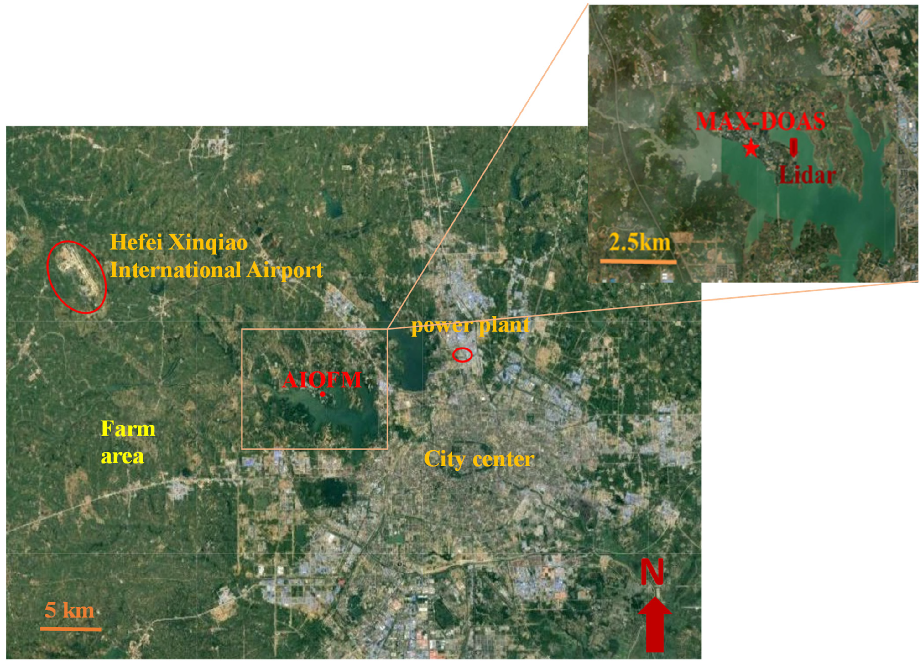
2.1. Site Description

The measurement site was situated on the campus of the Anhui Institute of Optics and Fine Mechanics (31.91°N, 117.16°E, 20 m), Chinese Academy of Sciences (AIOFM, CAS), located on Science Island, a suburban area of Hefei in Anhui Province, China. Figure 1 illustrates the location of the measurement site in relation to the surrounding topography. Additionally, Figure 1 displays relationship between the site’s MAX-DOAS and Lidar. Farm areas are in the north, west, and northeast, whereas areas in the southeast are highly urbanized. Furthermore, there is an airport located in the northwest and a power plant in the northeast.

2.2. MAX-DOAS and Lidar Setup

The MAX-DOAS systems was positioned on the campus of the Anhui Institute of Optics and Fine Mechanics (AIOFM), specifically on the roof of a 6-storey building. The spectrometer used in the MAX-DOAS measurements was a Princeton Instruments (PI) 160 (IsoPlane-160, Princeton, USA), which was equipped with an area array of charge-coupled device (CCD) detectors, comprising 2048 $\times$ 512 pixels (Acton, Princeton, USA). The wavelength range of the spectrograph was from 290 to 410 nm, with a spectral resolution of 0.35 nm. The telescope restricted the field of view angle to less than 0.2°. During the measurements, the sequential elevation angles (EAs) were set at 1°, 2°, 3°, 4°, 5°, 6°, 8°, 15°, 30°, and 90°. Each individual measurement consisted of an average of 100 spectral recording scans, with the integration time automatically adjusted to optimize the signal-to-noise ratio based on the light intensity. The duration of each sequence of observations at 10 EAs was approximately 10 min. The system generally operated between the local time (LT) hours of 6:00 and 18:00. The MAX-DOAS data from an azimuth of 0° (north) were used for analysis in this study. A detailed description of the instrument can be found in Ren et al. [27].

A differential absorption Lidar was operated to retrieve aerosol extinction (AE, 316 nm) and O₃ profile at the Science Island Experimental Field, which was located approximately 1.0 km away from the MAX-DOAS (red rectangle point in Figure 1). The Lidar system employed in this study was developed by the AIOFM [28]. The maximum statistical error associated with the Lidar profile was found to be below 10% [29]. The assumed radar ratio for the measurements was set at 50 sr. Due to the observation blind spot of the Lidar, the aerosol profiles with altitudes of ≥0.3 km were used [27].

2.3. DOAS Analysis and Profile Retrieval

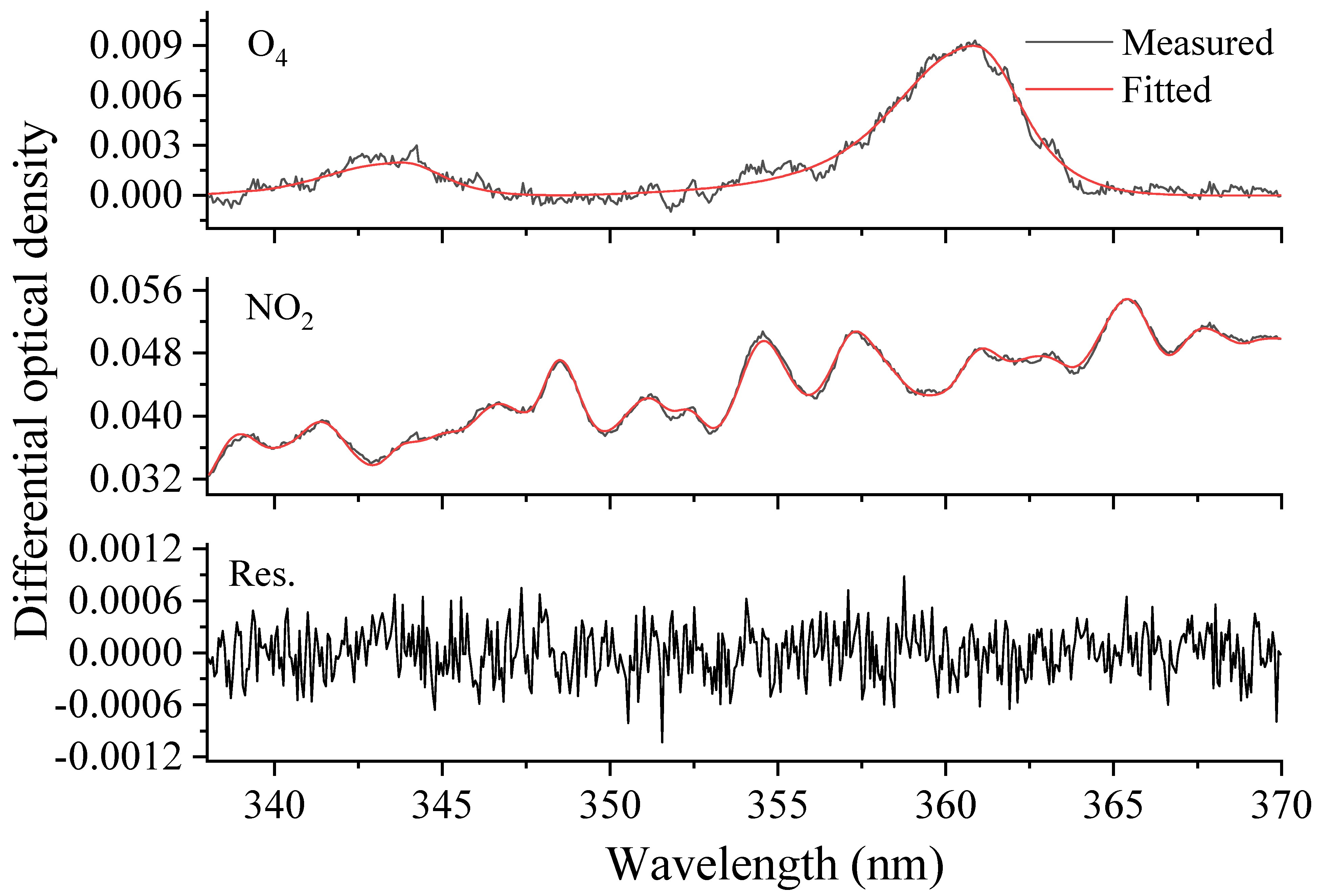
2.3.1. Spectral Analysis

Spectra were analyzed using the QDOAS software (http://uv-vis.aeronomie.be/software/QDOAS/ (accessed on 13 November 2023)) developed by BIRA-IASB. The O₄ and NO₂ dSCDs were retrieved in the spectral fitting window of 338–370 nm, which included several strong absorption bands. The measured Fraunhofer spectrum in the zenith was used as the reference spectrum for each cycle to eliminate the impact of the Fraunhofer reference spectrum (FRS) [1]. The parameter settings and the trace gas absorption cross-sections for the retrieval of NO₂ dSCDs were based on recommendations from the CINDI-2 campaign (2nd Cabauw Intercomparison of Nitrogen Dioxide-measuring Instruments, 2016 [30]), as shown in

Table 1. Baseline DOAS analysis settings used for the O₄ and NO₂ slant column retrieval, where “√” expresses the cross-section used in the retrieval.

Parameter	Source	Species
		O4 and NO2
Fitting spectral range		338–370 nm
NO2 (220 K, 294 K)	[31], I0-corrected (1017 molec. cm−2)	√
O4 (293 K)	[32]	√
O3 (223 K, 243 K)	[33], I0-corrected (1020 mole. cm−2)	√
HCHO (297 K)	[34]	√
BrO (223 K)	[35]	√
Ring		RING_DOAS_SAO2010 [36]
Polynomial degree		Order 5 (6 coefficients)
Intensity offset		Constant

. An example of an O₄ and NO₂ fitting result, which was obtained from these 2D MAX-DOAS on 4 September 2020 at a 1° EA and at 7:45 LT (local time), is shown in Figure 2. The typical root mean square error (RMSE) for NO₂ and O₄ was <0.001.

2.3.2. Profile Retrievals

The dSCD obtained from the DOAS spectral analysis represents the trace gas concentration along the effective optical path length. Thus, the dSCD must be converted to vertical column density (VCD) by applying the air mass factor (AMF) as follows:

$$\mathrm{V}\mathrm{C}\mathrm{D}=\frac{\mathrm{S}\mathrm{C}{\mathrm{D}}_{\mathrm{i}}-\mathrm{S}\mathrm{C}{\mathrm{D}}_{\mathrm{i}=90°}}{\mathrm{A}\mathrm{M}{\mathrm{F}}_{\mathrm{i}}-\mathrm{A}\mathrm{M}{\mathrm{F}}_{\mathrm{i}=90°}}=\frac{\mathrm{d}\mathrm{S}\mathrm{C}{\mathrm{D}}_{\mathrm{i}}}{\mathrm{A}\mathrm{M}{\mathrm{F}}_{\mathrm{i}}-\mathrm{A}\mathrm{M}{\mathrm{F}}_{\mathrm{i}=90°}},$$

(1)

where i represents the elevation angle.

VCD is defined as the integrated concentration of trace gas concentration through the atmosphere along a vertical path. AMF is often used to describe the absorption path of a gas in the atmosphere. The atmospheric RTM is able to calculate the AMF.

In this study, the PriAM algorithm, based on the SCIAMACHY radiative transfer model (SCIATRAN), which was used to retrieve trace gas VCDs and profiles, was developed by the Anhui Institute of Optics and Fine Mechanics, Chinese Academy of Sciences (AIOFM, CAS), in cooperation with the Max Planck Institute for Chemistry (MPIC) [24,37,38]. PriAM also consists of a two-step inversion procedure based on the optimal estimation method (OEM) [8,18,22,27,39]. PriAM can retrieve trace gas and aerosol profiles for any arbitrary vertical grid. In this study, vertical layers (altitude grid) with a 200 m resolution at an altitude range below 4.0 km were used. Parameter settings used in the general PriAM retrieval for aerosol and NO₂ profiles are shown in

Table 2. Parameter settings used in the general PriAM retrieval for aerosol and NO₂ profiles.

Parameters
Type of radiative transfer model	Scattered light in a spherical atmosphere
Vertical resolution	200 m resolutions at an altitude range below 4.0 km
A priori profile	Aerosol: Boltzmann shape with an AOD of 0.3 and a height of 1.5 km (See Table S1 for details) NO2: Boltzmann input profile with a NO2 VCD of 1.0 × 1016 molec. cm−2 (See Table S1 for details)
Wavelength (nm)	360
Single scattering albedo (SSA)	0.9
Asymmetry parameter (AP)	0.72
Surface albedo	0.06
Solar zenith angle (SZA, °)	From observation
Relative azimuth angle (RAA, °)	From observation
Azimuth angle (°)	0 (North)

.

In the OEM, the impact of the deviation between the retrieved profile and the true profile, caused by the retrieval profile shifting towards the a priori profile at a higher altitude [17], is referred to as the “smoothing effect”. Information about the vertical resolution and sensitivity is provided by the averaging kernel matrix (AVK). The trace of AVK is equivalent to the degrees of freedom for signal (DOFS), which quantifies the total number of independent pieces of information contained in the measurements compared to the a priori one. The maximum value of the AVK for each layer can represent the sensitivity for that specific layer in the retrieval. The envelope, formed by connecting the maximum AVK values of each layer, illustrates the change in sensitivity with height. In this study, the height corresponding to an envelope value decreasing to 10% of the maximum value is termed the upper sensitive height limit (H_m). An altitude range of 0 to H_m is considered the sensitive zone for profile retrieval by MAX-DOAS.

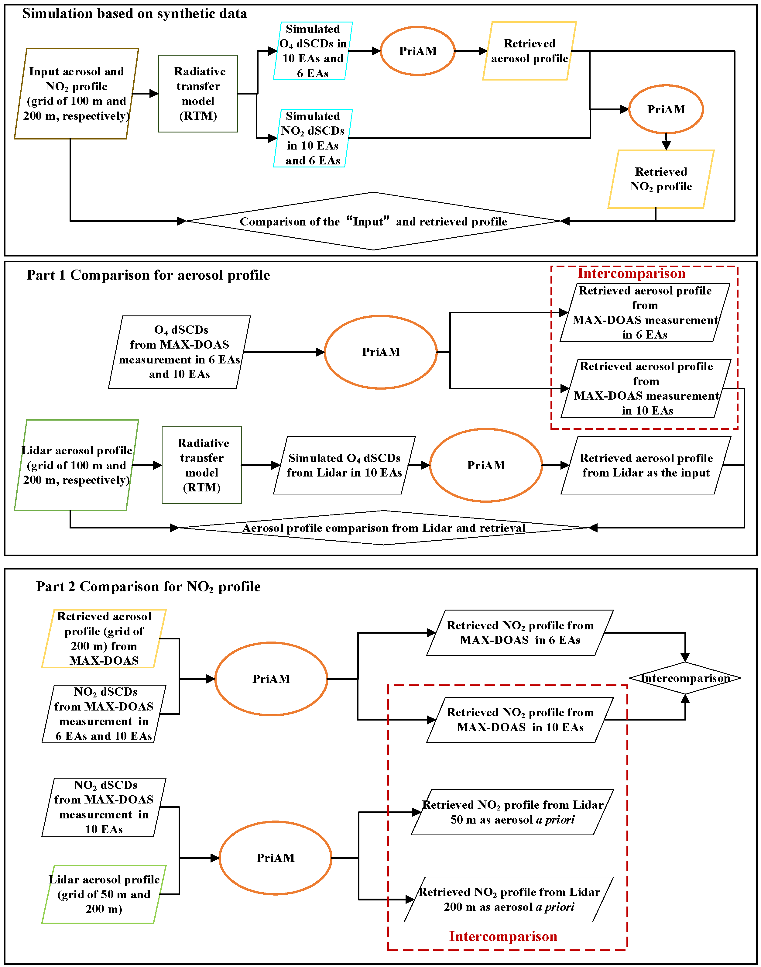
2.4. Analysis Strategy and RTM Parameters

This study employed both simulations and actual measurements to verify the impact of the vertical resolution of the input profile and the elevation angle on the retrieved trace gas profile. The depicted analysis strategy in Figure 3 outlines the approach. Firstly, the simulation focused on assessing the effect of the vertical resolution of the input profile and EAs on the retrieved profile using synthetic data. The vertical resolution of the input profile was set to 100 or 200 m. AOD and NO₂ VCD were set to 0.3 and 1.0 $\times$ 10¹⁶ molec. cm⁻², respectively. O₄ and NO₂ dSCDs were calculated from input profiles by RTM, which were then used in aerosol and NO₂ profile retrievals. The retrieved and input profiles were subsequently compared. It is important to note that aerosols influence NO₂ profile retrieval. When using the two-step inversion algorithm PriAM to retrieve the NO₂ profile, the a priori aerosol profile information was obtained from the aerosol profile at a 200 m resolution input. Secondly, the study utilized MAX-DOAS and Lidar observations to validate the simulation results. Part 1 focused on verifying the effect on aerosol profile retrieval: (1) the impact of different EAs on aerosol profile retrieval was investigated; (2) aerosol profiles observed by Lidar with different vertical resolutions were used as input profiles, and the aerosol profiles were then retrieved following the simulation strategy. The retrieved aerosol profile with the Lidar profile as input was compared with the aerosol profile from the MAX-DOAS and Lidar observations. Part 2 addressed the verification of the effect on NO₂ profile retrieval: (1) the influence of different EAs on NO₂ profile retrieval was examined; (2) the retrieved NO₂ profiles were compared under the a priori aerosol profiles from the scenarios of the MAX-DOAS and Lidar observations.

In this study, the SCIATRAN version 2.2 [39] was utilized for the forward model calculations, consistent with PriAM. The EAs were configured for four scenarios: 10 EAs for Setting I (i.e., 1, 2, 3, 4, 5, 6, 8, 15, 30, and 90°), aligning with the MAX-DOAS measurement settings; the low EAs were reduced for Setting II, with six EAs (i.e., 2, 4, 8, 15, 30, and 90°); the low EAs were retained for Setting III, with six EAs (i.e., 1, 2, 3, 4, 5, and 90°); and the low EAs were omitted for Setting IV, with six EAs (i.e., 5, 6, 8, 15, 30, and 90°). In the simulation of synthetic data and real atmospheric inversion, the scenario with a single scattering albedo (SSA) = 0.9, asymmetry parameter (AP) = 0.72, and surface albedo = 0.06 was used in the simulation. These values were the long-term averages from the Aerosol Robotic Network (AERONET) at the Hefei site [37,40]. A solar zenith angle (SZA) = 60° and relative azimuth angle (RAA) = 120° were also applied in the simulation of synthetic data. In the real atmospheric inversion, the SZA and RAA were derived from actual measurements. Three profile shapes were employed in the simulation, which are exponential, Boltzmann, and Gaussian shapes. Exponential profiles depict a systematic decrease in concentration with altitude, representing situations where emissions typically occur at the surface. Boltzmann profiles signify situations typical for well-mixed boundary layers. Gaussian profiles illustrate scenarios involving pollutant transport, which typically occurs above the boundary layer. In this study, a Boltzmann profile corresponding approximately to the boundary layer height and a Gaussian profile representing pollutant transport in the boundary layer were designed. The detailed parameters used for the RTM in the simulation are presented in Table S1.

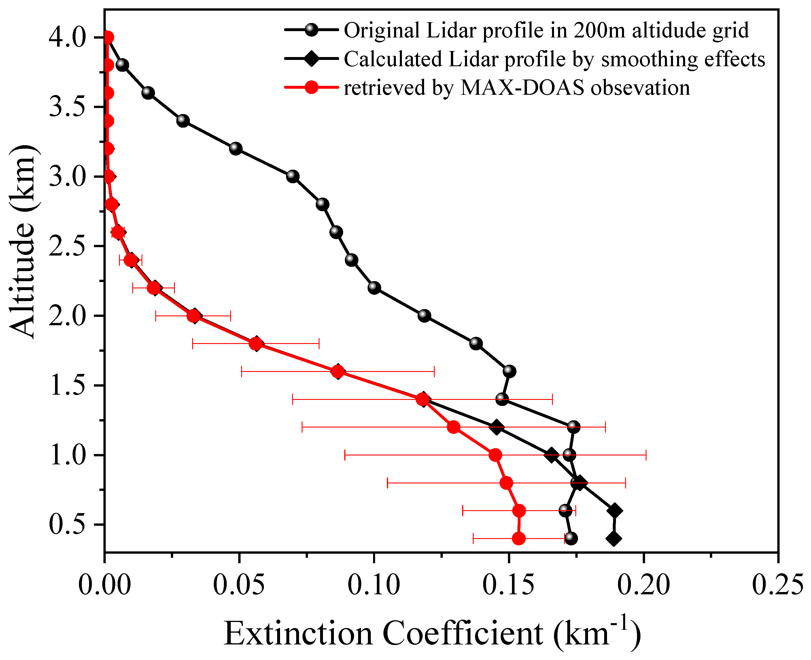
2.5. Pretreatment of Lidar Aerosol Profiles

Before comparing the Lidar aerosol profile with the MAX-DOAS retrieval result, the Lidar aerosol profile needed to be preprocessed to match the vertical resolution of the MAX-DOAS result. Firstly, as the aerosol extinction measurements were acquired by two different systems operating at distinct wavelengths (MAX-DOAS: 360 nm; Lidar: 316 nm), the Lidar’s extinction profiles needed to be converted to the MAX-DOAS wavelength using the aerosol Ångström exponent. The conversion was performed as follows:

$$(\frac{{\lambda }_a}{{\lambda }_b}{)}^{-\alpha }=\frac{\tau \left({\lambda }_a\right)}{\tau \left({\lambda }_b\right)},$$

(2)

where $\lambda$ and $\alpha$ represent the wavelength and Ångström exponent, respectively. $\tau \left(\lambda \right)$ denotes the aerosol optical depth. The Ångström exponent was derived from real-time observation data obtained by the Cimel Electronique sun photometer (CE318) located approximately 7 m away from the MAX-DOAS system. The wavelength range used for calculating the Ångström exponent ranged from 440 to 870 nm. Secondly, the vertical layer of the Lidar aerosol profile was processed into three altitude grids of 50, 100, and 200 m. Lastly, the gas and aerosol profiles were both smoothed in the OEM profile inversion algorithm retrieval. To reduce possible sources of discrepancies in the comparison of an OEM retrieved profile and Lidar profile, the Lidar profile resolution and information content had to be degraded by “smoothing” it with the corresponding MAX-DOAS AVK matrix (A) according to the following equation [17]:

$$\tilde{x}=\mathbf{A}x+(1-\mathbf{A})xa,$$

(3)

Here, $x_a$ is the a priori profile; $\tilde{x}$ represents the profile smoothed by the MAX-DOAS AVK matrix A; $x$ perfectly represents the Lidar profile.

3. Results and Discussion

The MAX-DOAS profile inversion algorithm establishes a functional relationship between the measurement vector and parameters of the atmospheric state based on the RTM. The optimal state between the measurements and prior values for the aerosol and gas was calculated by linear and nonlinear iteration. In order to investigate the effect of the observation information on the MAX-DOAS profile retrieval, the simulation of synthetic data and the verification of actual observations were adopted. Specifically, the number of elevation angles and the vertical resolution of the input profiles were used to represent different observation information obtained by MAX-DOAS.

3.1. Aerosol Results

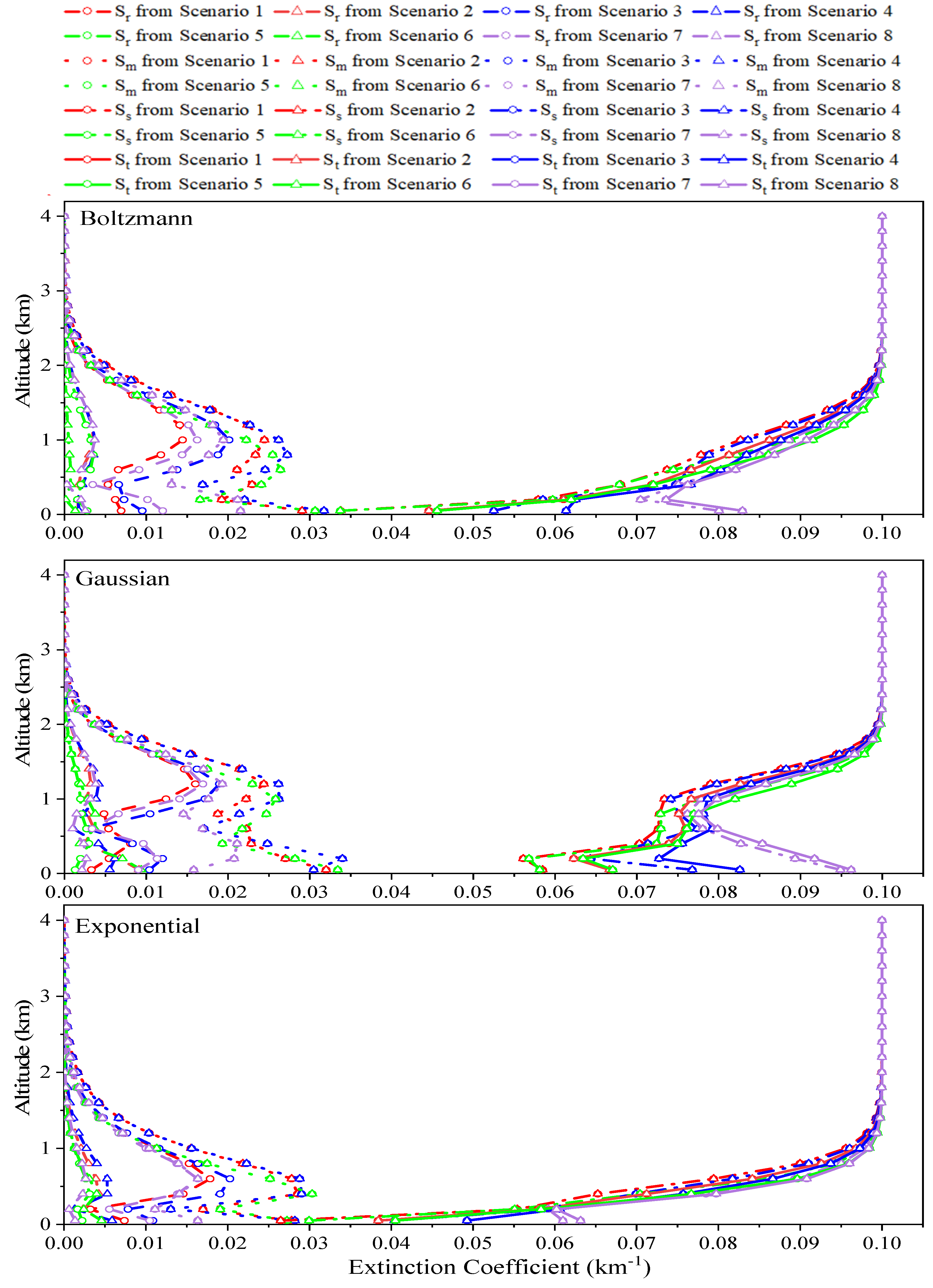
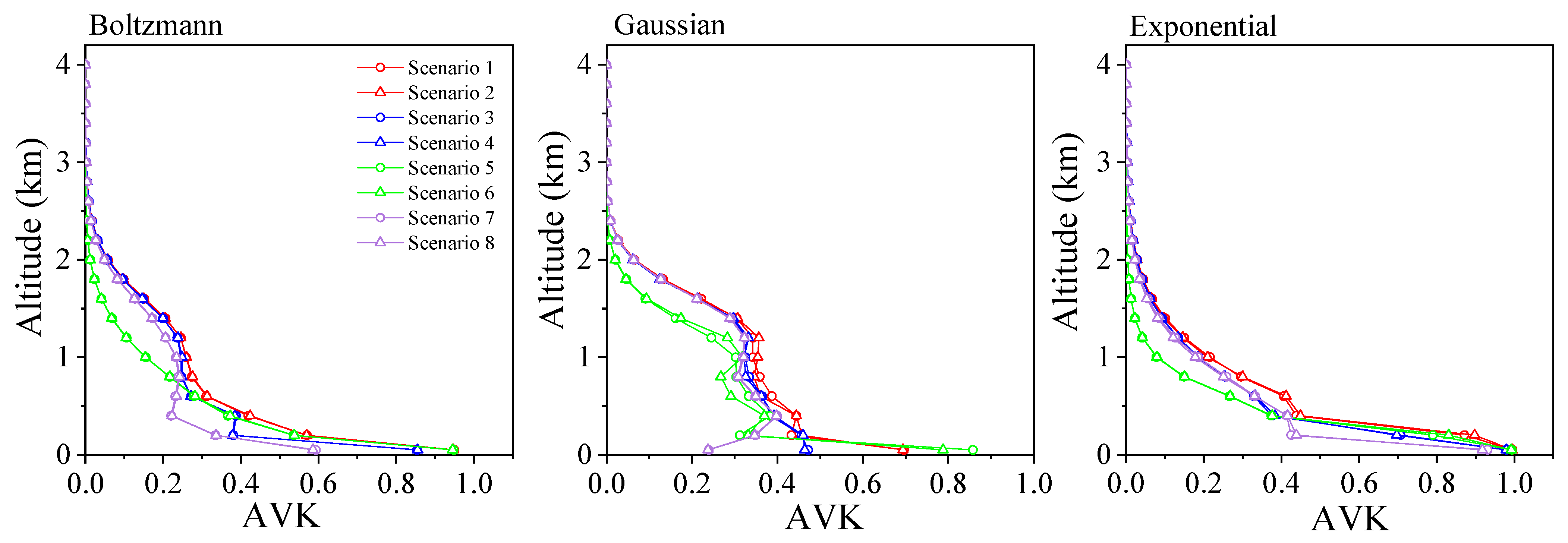
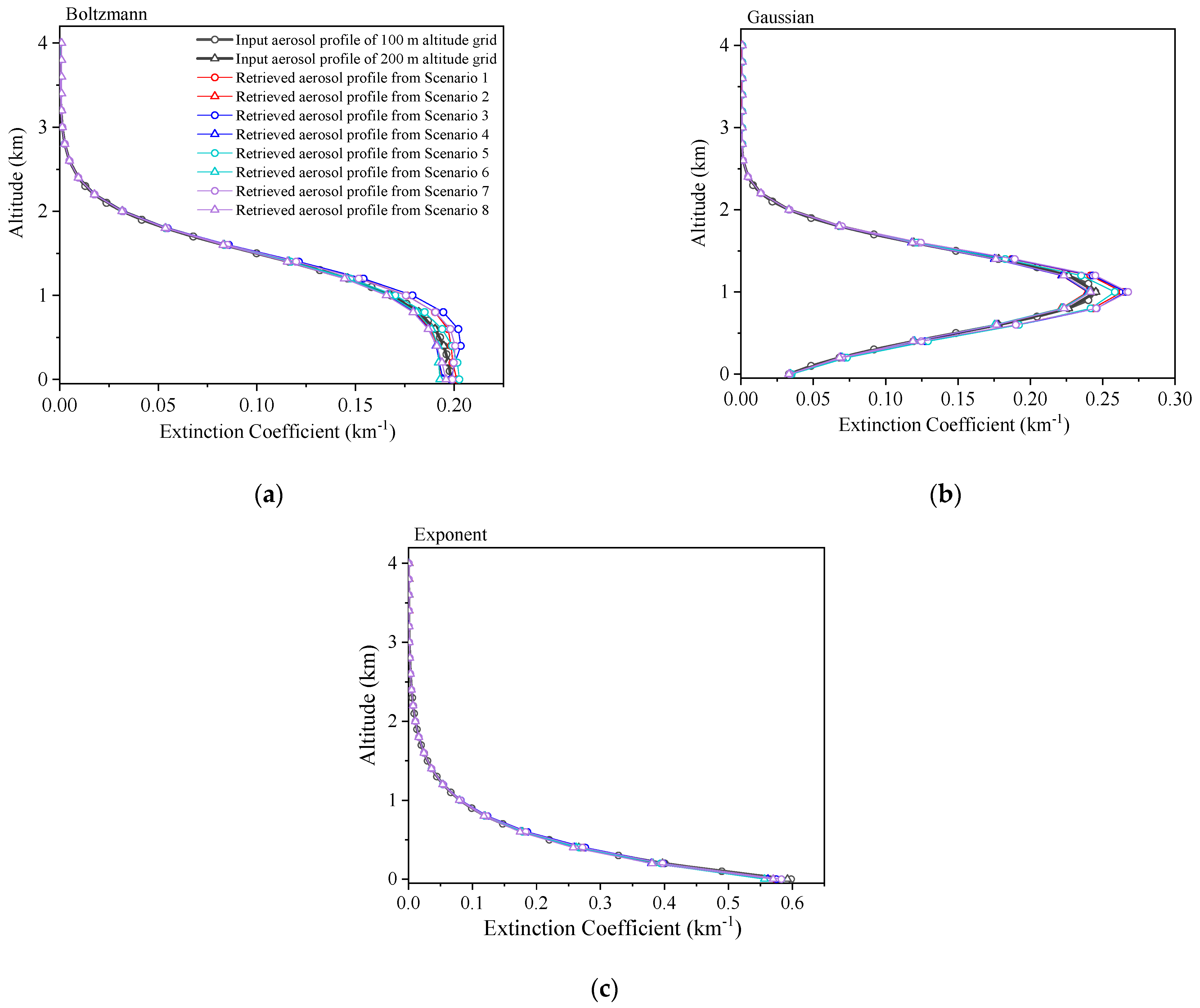
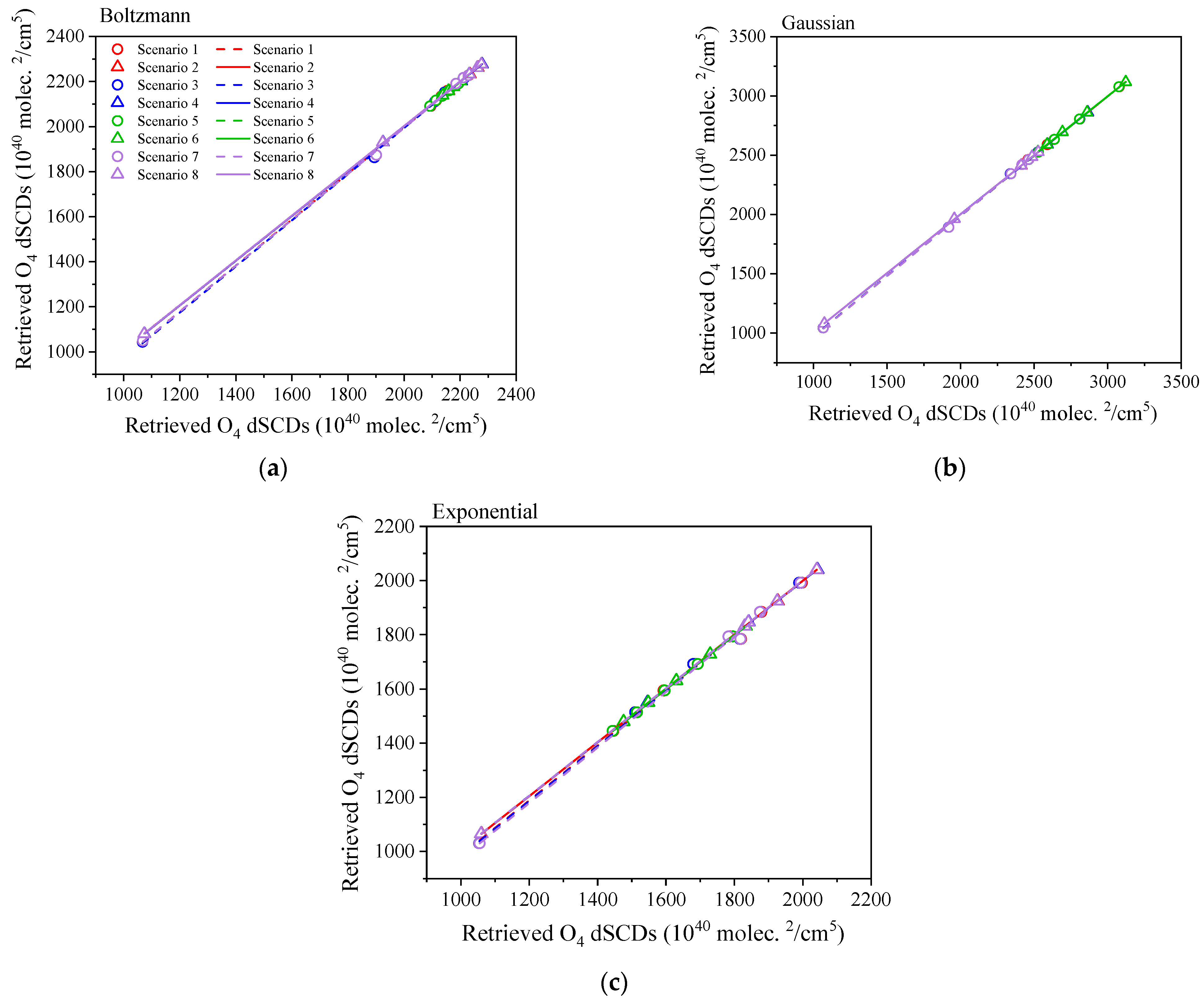
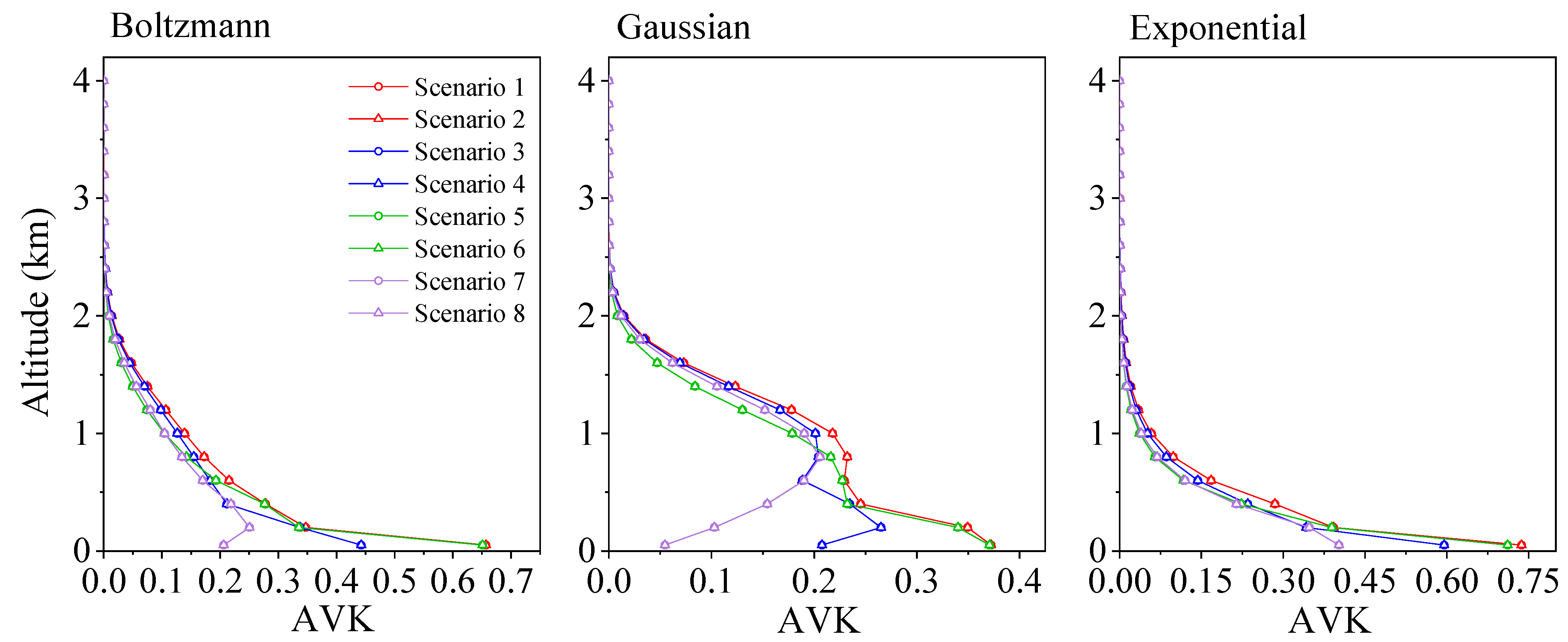
3.1.1. Effect on the Aerosol Profile Retrieval

Aerosol profiles with the same concentration but varying resolutions serve as representations of the diverse MAX-DOAS observation information. Consequently, these aerosol profiles were used to simulate the effect of MAX-DOAS observation information on aerosol profile retrievals. The input aerosol profiles were configured with vertical resolutions of 100 m and 200 m. Initially, the O₄ dSCDs were simulated using the RTM based on the “assumed input aerosol profiles” with different vertical resolutions, while considering various settings of EAs. Subsequently, the simulated O₄ dSCDs were used as inputs in the PriAM algorithm for retrieving the aerosol profile.

The aerosol profiles retrieved from various scenarios are depicted in Figure 4. In general, the retrieved aerosol profile from all scenarios at an AOD of 0.3 closely approximated the input aerosol profile. However, the retrieved aerosol profiles from a 100 m resolution as input exhibited slight differences compared to those from 200 m as input. Moreover, the retrieved scale height of the aerosol profile in a Boltzmann shape from 100 m resolution as input was slightly higher than that from 200 m as the input profile. The aerosol profiles retrieved using a 200 m resolution as input displayed an underestimation below 1.2 km, particularly for aerosol extinction below 500 m. In contrast, the aerosol profile results obtained using a 100 m resolution as input exhibited an overestimated trend below 1.2 km, primarily for aerosol extinction between 400 m and 1.0 km. The concentration value at the peak of the retrieved Gaussian shape profile from the 100 m resolution input was higher than the input value. Conversely, the concentration value from the 200 m resolution input was underestimated. It is worth noting that, for the retrieved exponential aerosol profile, the value in the first layer was underestimated in both resolutions used as input. In general, the aerosol profile below 2.0 km retrieved from a 100 m resolution input exhibited a slight overestimation compared to the input value. Conversely, the aerosol profile obtained from a 200 m resolution input showed a slight underestimation. However, the relative deviation in the 100 m resolution input was marginally higher than that in a 200 m resolution input. It is worth noting that the vertical resolution of the input profile does not have a significant effect on the shape of the retrieved profile. The retrieved aerosol profiles differed slightly among different EAs, particularly from a 100 m resolution input. When the aerosol profile with a 200 m resolution was used as the input, the difference between the retrieved results and the input value for EAs using Setting IV was minimal. However, the smallest deviation for the 100 m resolution input was observed in EAs utilizing Setting III. This is mainly due to the fact that low elevation angles contain more information with respect to gas profile shapes than high elevation angles [41].

The discrepancy between the simulated O₄ dSCDs by the PriAM algorithm and the input O₄ dSCDs (simulated using the RTM from the input aerosol profile) can serve as a metric to evaluate how PriAM effectively utilizes the measured aerosol information (Figure 5).

Table 3. The correlation coefficient (R), slopes, and intercepts of the linear regressions for O₄ dSCDs simulated by the PriAM algorithm and the input O₄ dSCDs in the eight scenarios. The scenarios correspond to Figure 4.

Shape	Parameters	Scenarios
		1	2	3	4	5	6	7	8
Boltzmann	Slope	1.02	0.9	1.02	0.99	0.97	1.00	1.02	0.99
	Intercept	−46.50	16.02	−54.86	13.69	60.41	4.91	−45.07	14.14
	R	1.000	1.000	1.000	1.000	0.999	1.000	1.000	1.000
Gaussian	Slope	0.99	1.00	1.02	0.99	1.00	0.99	1.02	0.99
	Intercept	21.16	12.99	−41.43	13.88	−8.61	34.46	−50.73	13.43
	R	1.000	1.000	1.000	1.000	1.000	1.000	1.000	1.000
Exponential	Slope	1.01	0.99	1.01	0.99	0.99	0.98	1.02	0.99
	Intercept	−27.62	13.44	−31.38	15.69	16.28	28.91	−50.72	14.33
	R	0.999	1.000	0.999	1.000	1.000	1.000	0.999	1.000

presents the correlation coefficient (R), slopes, and intercepts of the linear regressions for the eight scenarios. The O₄ dSCD simulated by PriAM closely approximated the input value, as evidenced by the fitting slope and correlation coefficient both approaching 1.00. The O₄ dSCDs calculated from the aerosol profiles of two resolutions based on the RTM were consistent, suggesting that SCITRIAN is capable of extracting similar information from aerosol profiles with resolutions of 100 m and 200 m.

In MAX-DOAS profile inversion, the retrieval error encompasses the smoothing error (S_s), measurement error (S_m), and residual error (S_r). The total error (S_t) of the inversion is calculated using the error transfer formula: ${\mathrm{S}}_{\mathrm{t}}=\sqrt{{\mathrm{S}}_{\mathrm{S}}^2+{\mathrm{S}}_{\mathrm{m}}^2+{\mathrm{S}}_{\mathrm{r}}^2}$. The retrieval can be regarded as an estimate of the true state that has been smoothed by the averaging kernel. Hence, the error contribution due to smoothing is termed the smoothing error. The error caused by the measurement of trace gas is referred to as the measurement error. The error from the value function is labeled the residual error. The retrieval errors for the aerosol profiles at different resolutions and EA settings are depicted in Figure 6. The S_m, S_s, and S_t remain largely constant for both resolutions, whereas there are slight variations among the four EA settings. The S_r changed due to the variations in resolutions of the input aerosol profiles and the number of EAs. The S_r of a 100 m resolution input was significantly higher than that of a 200 m input. This is why the retrieved aerosol profile from a 200 m resolution input was closer to the true value compared to that from a 100 m resolution input. The increase in S_r suggested that the value function could not be effectively minimized during the nonlinear iterative calculation. This demonstrates that the nonlinear solving process needs optimization to improve the accuracy of the inversion algorithm under high-resolution aerosol profiles. The lowest S_r value from the 100 m resolution input was recorded for Setting III with 6 EAs, whereas, for the 200 m resolution input, it was observed for Setting IV with 6 EAs. This aligns precisely with the retrieved results of the aerosol profile.

The gain in information on the atmospheric state can be quantified through the OEM retrieval, which is represented by the AVK matrix. Therefore, the information and sensitivity obtained by PriAM inversion were assessed under different vertical resolutions of the aerosol profile as input. In Figure 7, the retrieved envelopes of the AVK are presented for three different shapes. The corresponding values of H_m and DOFS are provided in

Table 4. The retrieved DOFS and H_m for three aerosol shapes from the eight scenarios. The scenarios correspond to Figure 4.

Shape	Parameters	Scenarios
		1	2	3	4	5	6	7	8
Boltzmann	DOFS	1.95	1.95	1.58	1.58	1.73	1.73	1.10	1.10
	Hm	1.4	1.4	1.6	1.6	1.2	1.2	1.6	1.6
Gaussian	DOFS	1.95	1.95	1.55	1.55	1.73	1.73	1.06	1.06
	Hm	1.6	1.6	1.8	1.8	1.6	1.6	1.8	1.8
Exponential	DOFS	1.66	1.66	1.38	1.38	1.46	1.46	1.05	1.05
	Hm	0.8	0.8	0.8	0.8	0.6	0.6	0.8	0.8

. The retrieved envelopes of the AVK, DOFS, and H_m from altitude resolutions of 100 m and 200 m as input were found to be in agreement. This suggests that the information obtained from both resolution profiles as input used in the PriAM retrieval process is consistent. Additionally, a decrease in the number of EAs resulted in a reduction in the retrieved envelopes of the AVK and DOFS, indicating that the maximum information gain from the measurements was achieved at 10 EAs. Therefore, despite the minimum deviation in the aerosol profile found at 6 EA retrieval, the EA setting with 10 EAs is still recommended, considering the small deviation and the uncertainty in the profile.

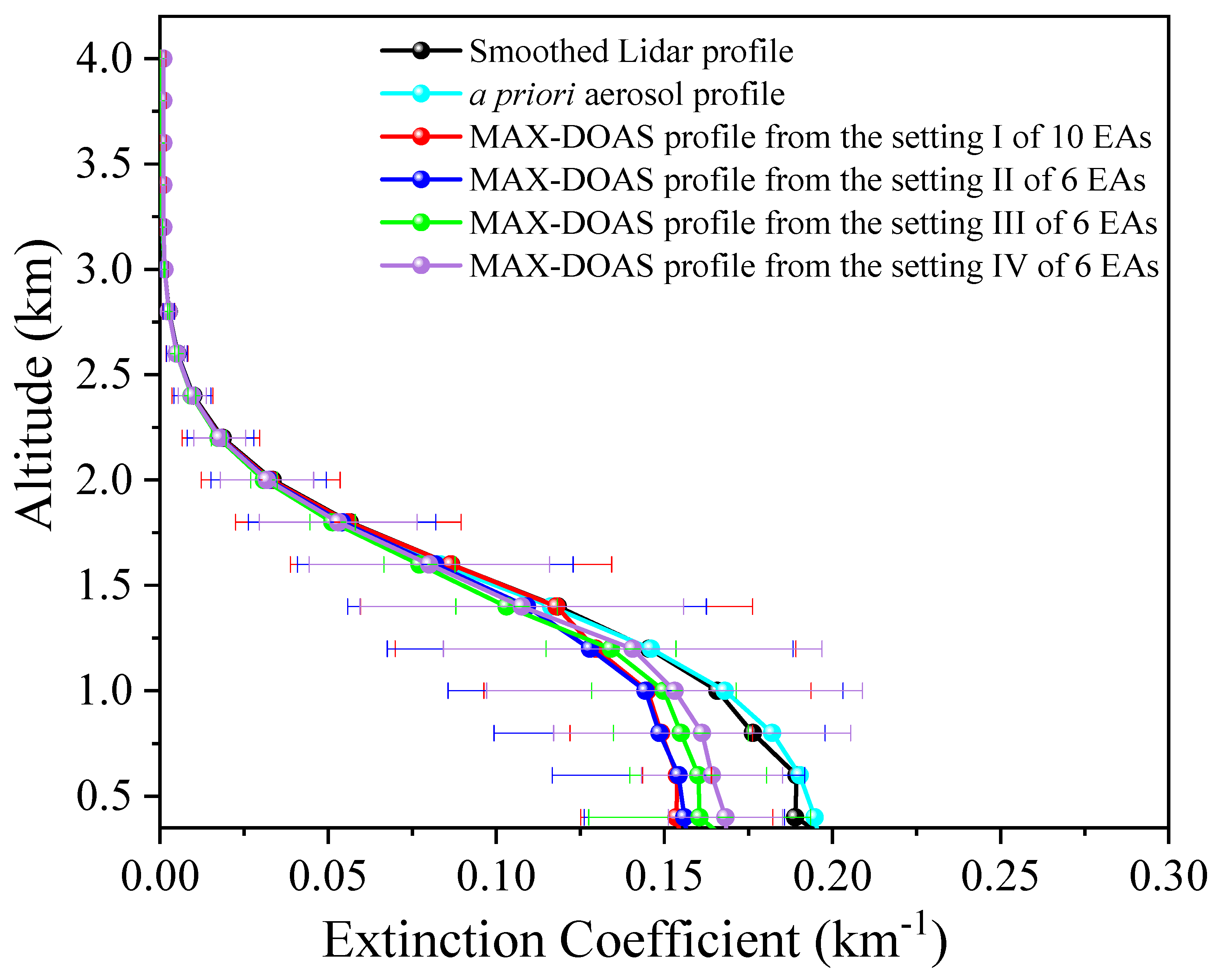
3.1.2. The Aerosol Profile Retrieval in MAX-DOAS Observations

In real MAX-DOAS measurements, the determination of gas concentration in the atmosphere relies on observations at various elevation angles. To ensure the accuracy of the simulation, different EAs were matched with corresponding observation accuracies. The impact of EAs on the retrieval profile’s accuracy was investigated, with Hefei’s MAX-DOAS observations using 10 EAs (1, 2, 3, 4, 5, 6, 8, 15, 30, and 90°) and a comparative study with 6 EAs in the simulation. The aerosol profile for Hefei on 4 September 2020 was retrieved using the PriAM algorithm presenting results at 8:00 LT (local time) in Figure 8. The input profile at a 200 m resolution with AOD of 0.3, as detailed in Table 2, served as the universal a priori aerosol profile in the PriAM retrieval. Results indicated that aerosol extinctions below 1.5 km retrieved by 6 EAs and 10 EAs differed significantly from the Lidar aerosol profile, with 6 EAs showing higher values than 10 EAs. Among the EA settings, the aerosol profile retrieved from Setting IV with 6 EAs closely matched the Lidar profile, consistent with the simulation results in Section 3.1.1. Overall, the aerosol results from MAX-DOAS at 8:00 LT tended to be underestimated compared to Lidar observations.

The retrieved envelopes of the AVK, H_m, and DOFS at 8:00 LT under different EA settings are shown in Figure 9. The DOFS obtained from the inversions using 10 EAs were higher than that from inversions using 6 EAs, indicating that the information obtained from 10 EAs was greater. The retrieved H_m from Setting III with 6 EAs was the lowest compared to other EA settings, suggesting that the retrieval result from settings with only low EAs is sensitive to pollution at low altitudes. AODs retrieved by MAX-DOAS in four scenarios were compared with Lidar-measured AODs (Figure 10), with Lidar AODs being the result of AVK smoothing based on the preprocessed aerosol profile. Retrieved AODs at 8:00 LT from four scenarios were lower than Lidar values. AODs retrieved from 6 EAs were closer to Lidar AODs than those from 10 EAs, although the differences between AODs from 10 EAs and 6 EAs were negligible. In general, retrieved AODs under different EAs were close, demonstrating consistent results. The retrieved DOFS from different EAs indicated that employing a greater number of EAs can obtain more information from observations, particularly from a number below a 5° elevation angle, mainly because the lowest elevations contain most information with respect to gas profile shapes [41].

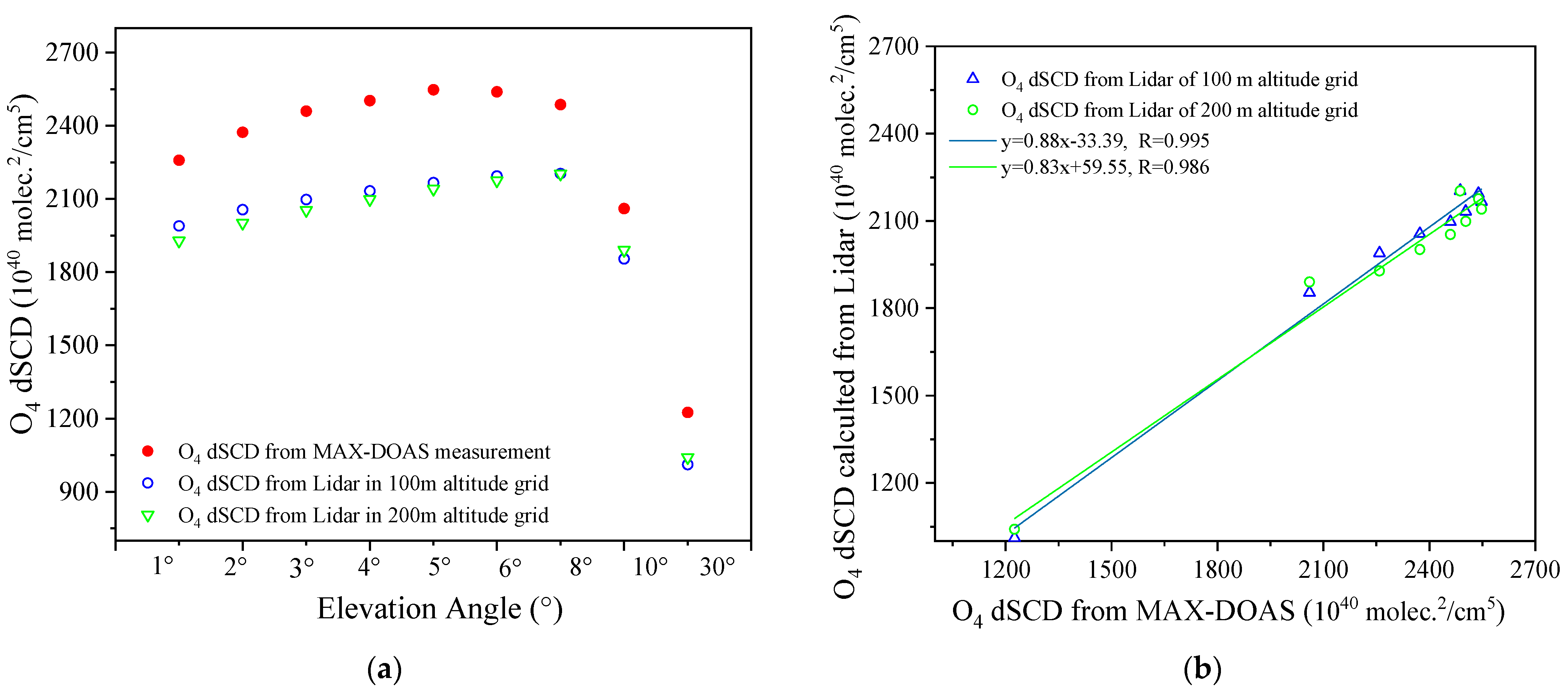
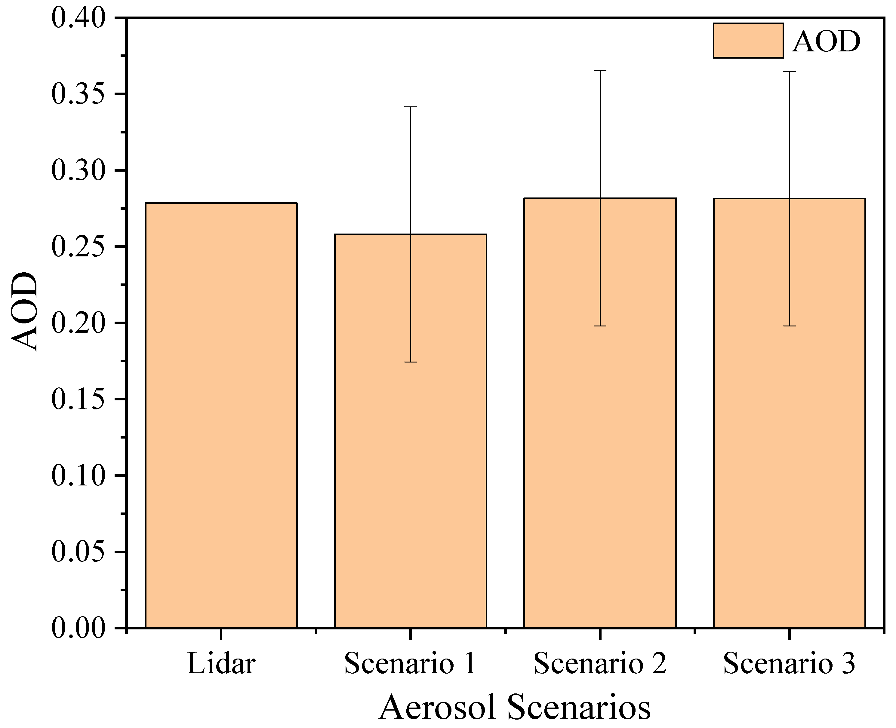
3.1.3. Lidar Results as the Input Aerosol Profile

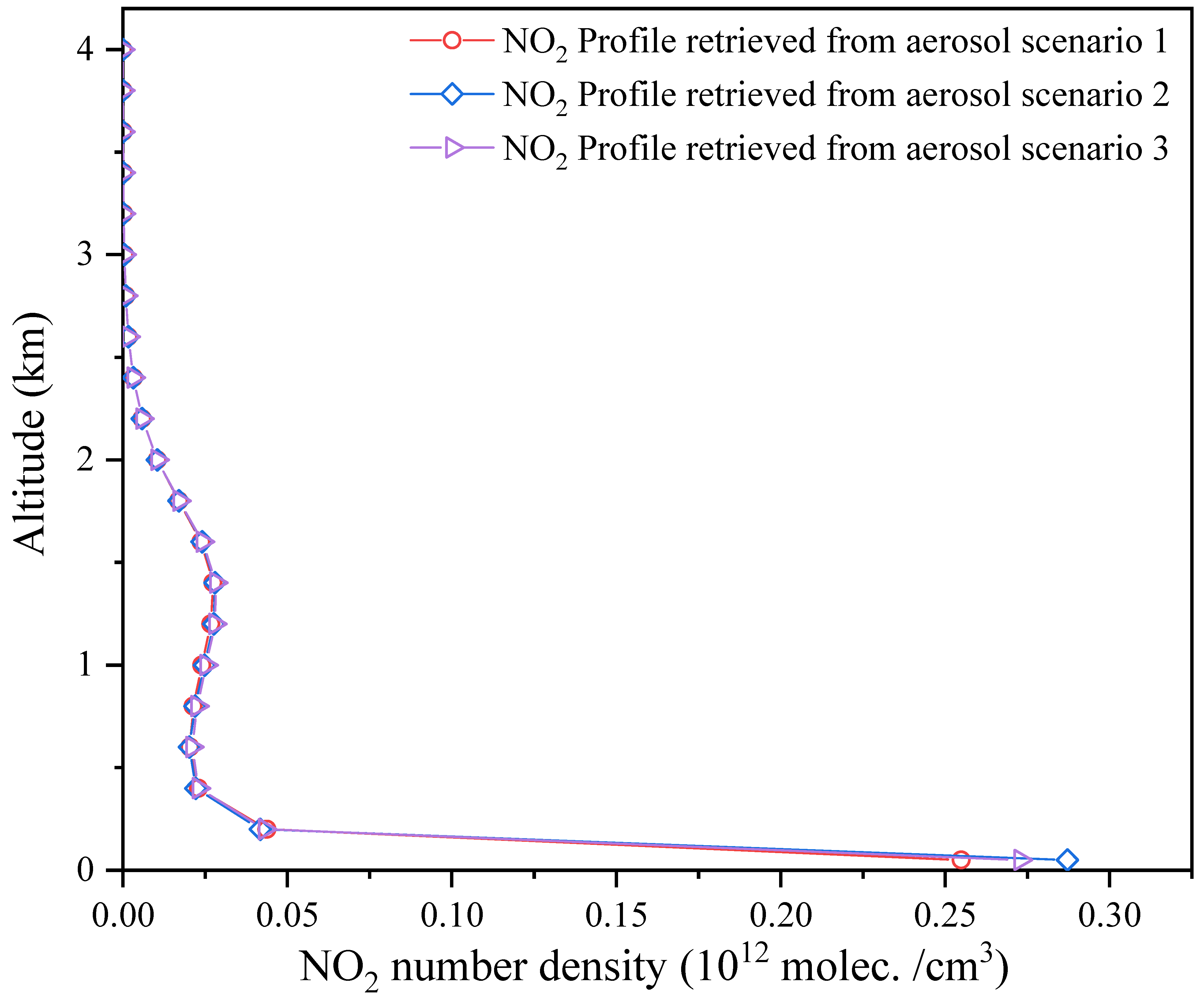
In the previous investigation, discrepancies were observed between the aerosol profiles retrieved from MAX-DOAS observations and the actual Lidar aerosol profiles. This disparity could be attributed to insufficient O₄ dSCDs information gathered by MAX-DOAS, leading to inconsistencies between MAX-DOAS inversion and Lidar observations. To explore this, Lidar aerosol profiles were utilized as input profiles in the RTM to calculate O₄ dSCDs. Subsequently, the aerosol profiles were retrieved using the calculated O₄ dSCDs by PriAM and compared with input Lidar profiles. Lidar aerosol profiles at 8:00 LT on 4 September 2020, at different vertical resolutions (i.e., 100 m and 200 m), were selected for simulation. Figure 11 illustrates a comparison between the input and retrieved aerosol profiles from Lidar profiles used as input profiles and from MAX-DOAS measurements at 10 EAs. The aerosol profiles retrieved from Lidar profiles at 100 m and 200 m vertical resolution inputs closely resembled the Lidar aerosol profiles, validating the consistency with the simulation results in Section 3.1.1. However, the aerosol profiles retrieved by MAX-DOAS measurements differed from those with Lidar profiles as input, indicating underestimation. This disparity might be due to (1) the influence of the AVK smoothing [19], (2) the different location and viewing geometry of MAX-DOAS and Lidar [18,42,43], and (3) uncertainties associated with the Lidar profiles. The original Lidar aerosol profiles at 8:00 LT and the retrieved aerosol profiles are displayed in Figure 12. The aerosol profiles retrieved by MAX-DOAS measurements demonstrated consistency with the original Lidar profile, albeit exhibiting significant differences in concentration, particularly above 1.0 km. These were close to the smoothed Lidar profile at altitudes exceeding 1.4 km. Moreover, the difference between the MAX-DOAS inversion results and the Lidar results can largely be explained by the smoothing effects. Figure 13 illustrates the correlation between the retrieved and input aerosol profiles. The correlation coefficient and slope between the Lidar aerosol profile and the retrieved aerosol profile from Lidar at 100 m and 200 m altitude resolution inputs were close to 1.0. The correlation coefficient between the MAX-DOAS measurements and the Lidar results surpassed 0.99, while the slope exhibited noticeable deviation.

To investigate whether the difference in aerosol profile retrievals was caused by the difference in O₄ dSCDs, the O₄ dSCDs simulated from Lidar profiles at two resolutions and those observed by MAX-DOAS were compared (Figure 14). The O₄ dSCDs calculated by the actual Lidar profile were lower than those from MAX-DOAS observations. The correlation coefficient of the O₄ dSCDs between the MAX-DOAS observations and Lidar simulation was higher than 0.98, with a slope greater than 0.83. The retrieval results based on the Lidar profiles at different resolutions were consistent with the simulation results in Section 3.1.1, further validating the conclusions of Section 3.1.1. That is, the inversion result from 100 m input overestimates the true value, while that from 200 m input is the opposite. The retrieved AODs from the three scenarios were compared with the smooth Lidar AOD (Figure 15). The AOD retrieved from MAX-DOAS observations was significantly underestimated compared with the AOD from the Lidar. The AOD retrieved by O₄ dSCD based on the actual Lidar profile simulation was also underestimated compared to the AOD from the Lidar, but the value was close. This shows that the accuracy of the aerosol information obtained by MAX-DOAS observations needs improvement, but the MAX-DOAS inversion algorithm can extract aerosol information from O₄ dSCDs effectively.

3.2. NO₂ Results

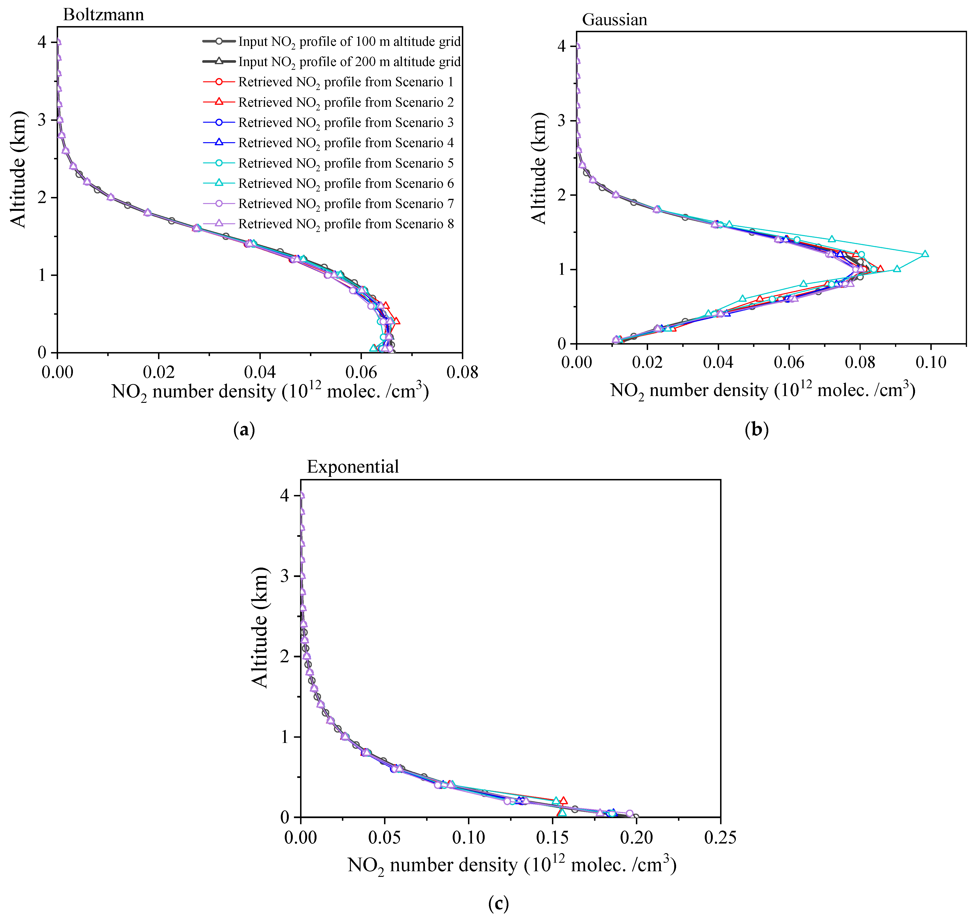
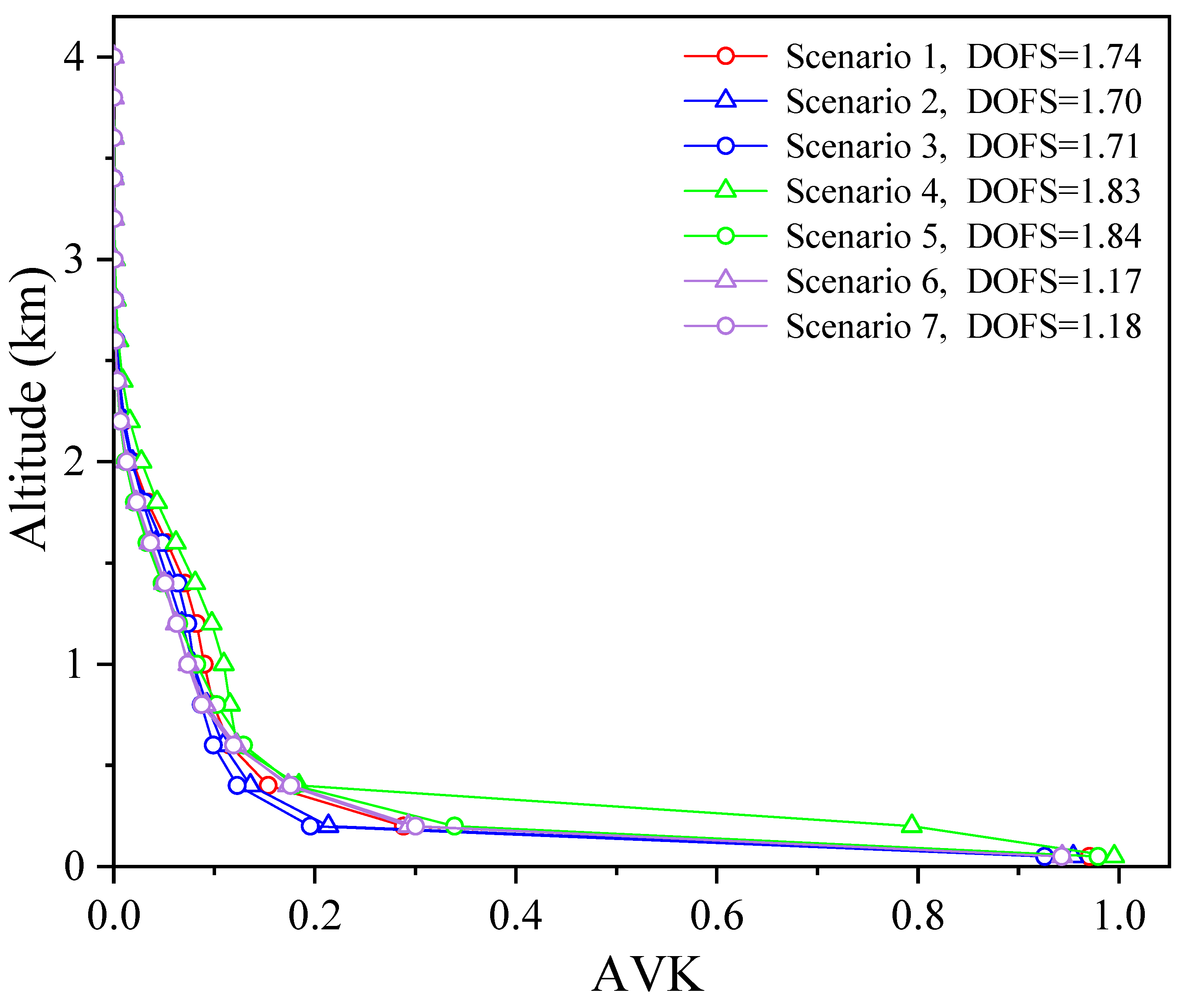
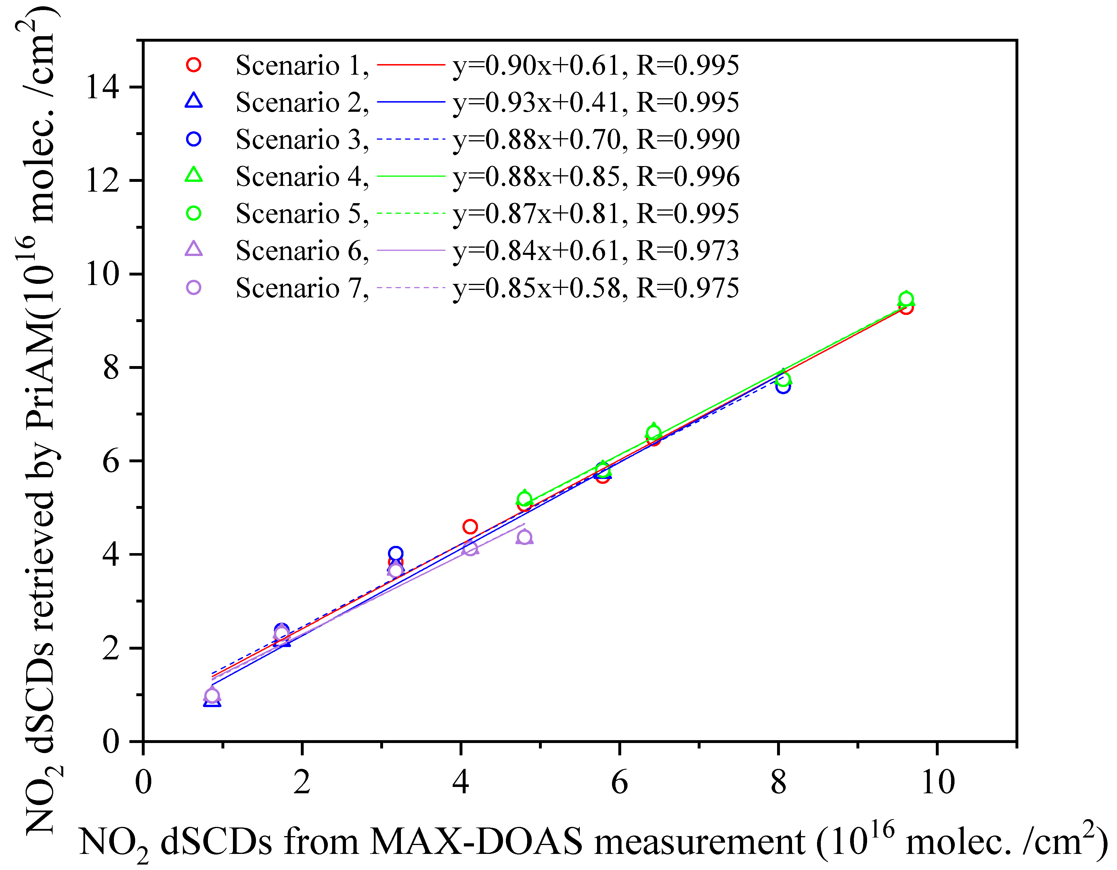
3.2.1. Effect of Vertical Resolution and Elevation Angles on NO₂ Profile Retrieval

The three selected NO₂ profiles were utilized for trace gas simulation under an AOD of 0.3. The NO₂ VCD was set to 1.0 $\times$ 10¹⁶ molec. cm⁻². Vertical resolutions of 100 m and 200 m were applied to the NO₂ profile. Additionally, the effect of EAs on NO₂ profile retrieval by MAX-DOAS was investigated. During the calculation of NO₂ dSCDs based on the RTM, the input aerosol profile, following a Boltzmann shape, with a vertical resolution of 200 m, served as the aerosol a priori profile. In comparison to aerosol inversion results, the retrieved NO₂ profiles based on the NO₂ profile with two vertical resolutions as input exhibited no significant overestimation or underestimation (Figure 16). The influence of vertical resolutions on NO₂ profile inversion appeared to be notably less pronounced than that observed in aerosol profile inversion. Similarly, and in line with the findings of aerosol inversion, the different EA settings had little impact on NO₂ profile retrievals. In summary, the impact of the input NO₂ profile’s vertical resolution and EA settings on NO₂ profile retrievals can be considered negligible.

The retrieved envelopes of the AVK, H_m, and DOFS under different scenarios were further compared (Figure 17 and

Table 5. The retrieved DOFS and H_m for three NO₂ shapes from the eight scenarios. The scenarios correspond to Figure 4.

Shape	Parameters	Scenarios
		1	2	3	4	5	6	7	8
Boltzmann	DOFS	3.16	3.17	2.74	2.74	2.52	2.52	2.11	2.11
	Hm	1.8	1.8	1.8	1.8	1.2	1.2	1.8	1.8
Gaussian	DOFS	2.91	2.91	2.45	2.46	2.17	2.16	1.97	1.97
	Hm	1.8	1.8	2.0	2.0	1.6	1.6	1.6	1.6
Exponential	DOFS	2.89	2.91	2.52	2.52	2.37	2.41	2.03	2.03
	Hm	1.4	1.2	1.2	1.2	0.8	0.8	1.2	1.2

). Under the same EA conditions, the retrieved envelopes of the AVK, H_m, and DOFS using input profiles with different altitude resolutions were essentially consistent. Similarly, the retrieved envelopes of the AVK, H_m, and DOFS at the same VCD scenarios exhibited consistency, indicating that AOD had minimal influence on NO₂ profile retrieval. The retrieved DOFS decreased as the number of EAs decreased, suggesting a reduction in the NO₂ information obtained from the observations as the number of EAs decreased.

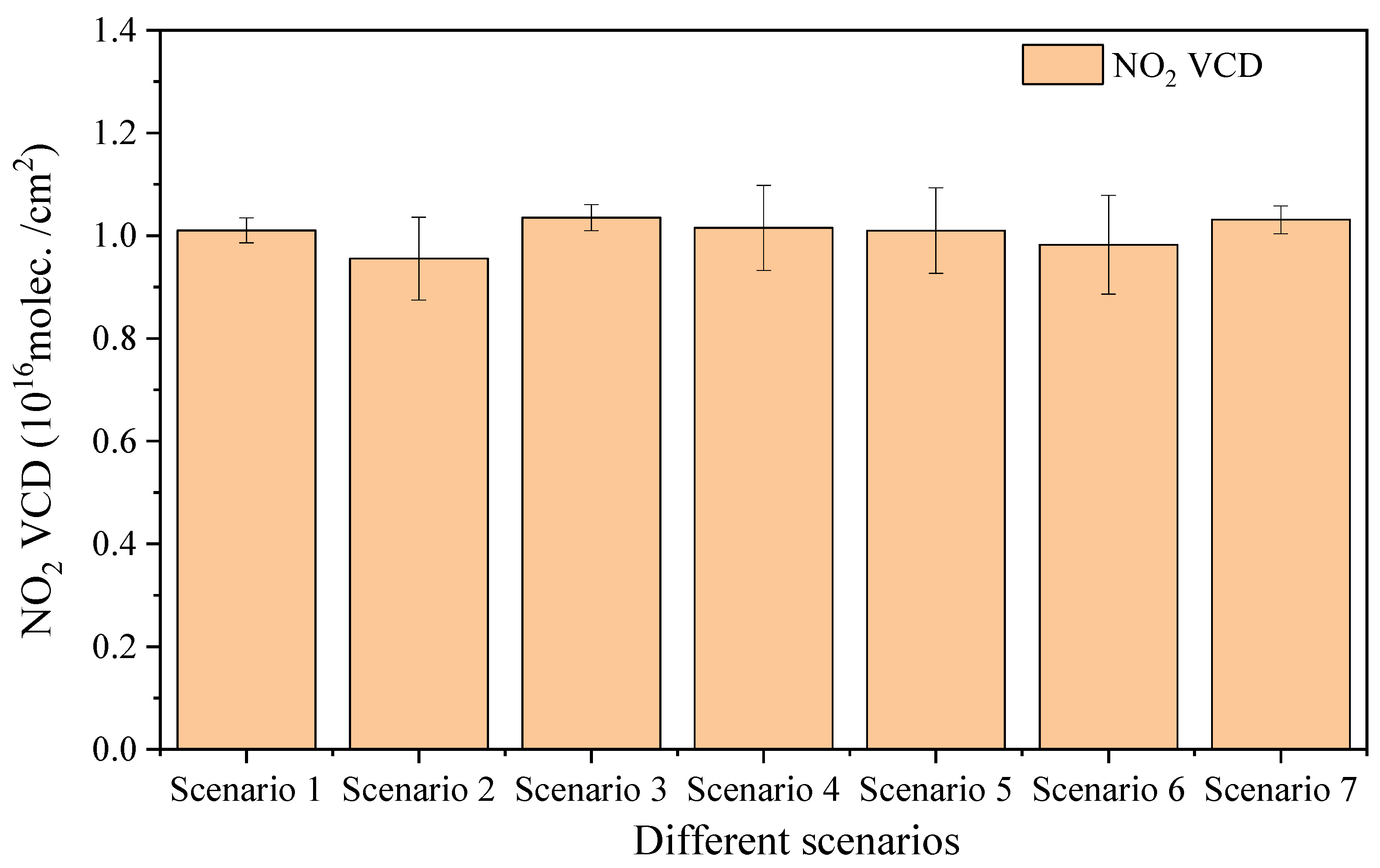
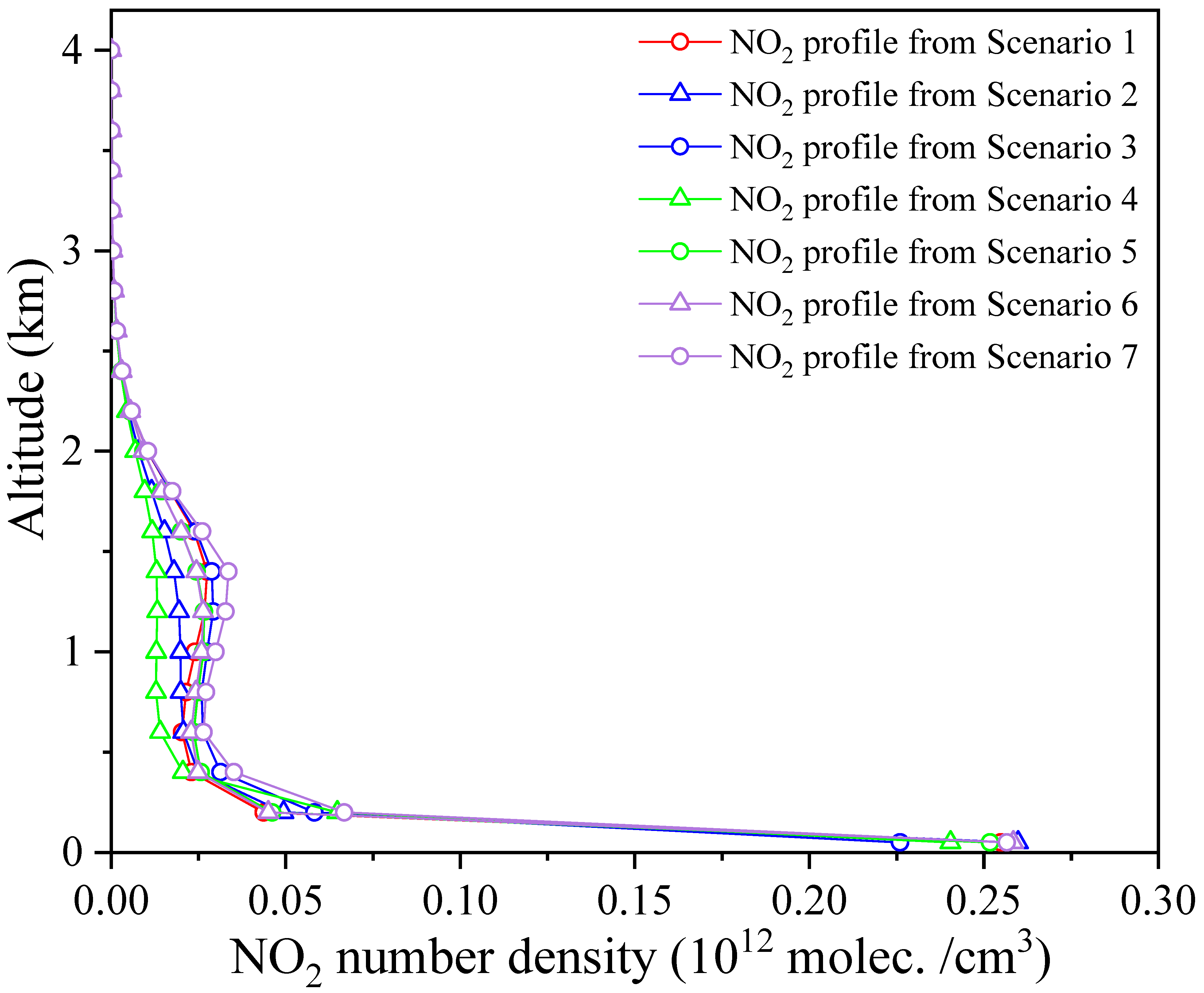
3.2.2. NO₂ Profile Retrieval in MAX-DOAS Observations

The study focused on evaluating the impact of EAs on NO₂ profile retrieval through MAX-DOAS observations. The a priori aerosol profile utilized in the retrieval process was derived from a total of 10 EAs. For NO₂ profile retrieval, the MAX-DOAS data collected at 8:00 LT on 4 September 2020 were employed. Figure 18 illustrates the influence of different EA settings on NO₂ profile retrieval, revealing slight variations, primarily within the altitude range of 400 m to 1.6 km. Specifically, the NO₂ number density retrieved with 10 EAs was marginally higher than that obtained with 6 EAs. Comparisons were made between NO₂ profiles retrieved from the a priori aerosol profiles corresponding to different EAs settings in the NO₂ inversion process (Figure 18). Minor differences were observed, particularly below an altitude of 2.0 km, where profiles retrieved with 6 EAs exhibited slightly higher values compared to those with 10 EAs. Nevertheless, these differences were deemed insignificant. Additionally, the NO₂ profiles retrieved from NO₂ and aerosols of the corresponding EAs were higher than those from aerosol profiles with 10 EAs.

Analyzing the retrieved envelopes of the AVK, H_m, and DOFS under various scenarios revealed consistent DOFS values from NO₂ with the same EA settings (Figure 19). This indicates that the PriAM algorithm’s ability to acquire gas information remains unaffected by the aerosol state. NO₂ VCDs retrieved from seven different scenarios are presented in Figure 20, showing a relative difference of less than 3%. Hence, the impact of EAs on NO₂ VCD retrievals can be considered negligible.

To assess the accuracy of NO₂ profiles retrieved by PriAM, the proximity of simulated NO₂ dSCDs to those measured by MAX-DOAS was crucial. Figure 21 demonstrates the comparison of NO₂ dSCDs simulated by PriAM under seven different scenarios with those measured by MAX-DOAS. The correlation coefficients exceeded 0.97, with a slope of 1 ± 0.15, indicating that the inversion algorithms effectively utilized information from MAX-DOAS observations.

3.2.3. Lidar Profiles as Aerosol Profiles in NO₂ Profile Retrievals

To verify the impact of vertical resolutions in aerosol profiles on NO₂ profile retrievals, Lidar profiles with vertical resolutions of 50 m and 200 m were employed as aerosol information in the PriAM algorithm for NO₂ profiles retrieval. The same MAX-DOAS data used in Section 3.2.2 were utilized for NO₂ profile retrieval. NO₂ profiles were retrieved by PriAM based on aerosol profiles obtained from both MAX-DOAS retrievals and Lidar measurements (Figure 22). The results indicated that the effect of vertical resolutions for the Lidar profiles as aerosol information on NO₂ profile retrieval was insignificant. This finding aligns with previous reports [22], confirming that the retrieved NO₂ profiles were consistent based on the input aerosol profile and the retrieved aerosol profile.

3.3. Discussion

While the verification relied on the results from the MAX-DOAS observation at 8:00 LT on 4 September 2020, encompassing only one day, it is crucial to note that diverse scenarios were explored for aerosol and NO₂ retrievals through synthetic data simulation. The findings from the actual measurements aligned with those derived from synthetic data simulation, although it is essential to acknowledge that synthetic measurements represent an idealized scenario and disparities between true and retrieved states may be more pronounced in actual atmospheric measurements [18]. On one hand, real-world atmospheric inhomogeneities, particularly clouds in the observation EAs, can exert a significant influence on MAX-DOAS measurements. On the other hand, in actual atmospheric retrieval, while the conclusion regarding the impact of EAs and vertical resolutions on inversion remains consistent with the simulation results, the relative deviation between the retrieval and true values depends on the shape and concentration of the gas profile and the a priori profile. Nonetheless, the vertical resolution of the input profile has a relatively insignificant effect on the shape of the retrieved profile. Specifically, when dealing with particularly high uplifted layers, the retrieval results using Setting III with 6 EAs exhibit a notable underestimation of the height and concentration of the uplifted layer. A study by Vlemmix et al. (2011) highlighted that accurate retrieval of NO₂ is achievable in a homogeneously mixed boundary layer; however, accurate measurement and precise aerosol extinction information are imperative for retrieving NO₂ in the free troposphere [41]. Considering the DOFS obtained from both simulation and measurement, it is advisable to prioritize Setting I with 10 EAs.

4. Conclusions

The study focused on exploring the impact of vertical resolution and elevation angles on NO₂ and aerosol profile retrievals through a combination of simulation and measurements. In the simulation, three shapes—Boltzmann, Gaussian, and exponential—were employed for aerosol and NO₂ profile retrievals. The vertical resolutions of the input profiles were set at 100 and 200 m, while fixed values for AOD and NO₂ VCD were 0.3 and 1.0 $\times$ 10¹⁶ molec. cm⁻², respectively. The aerosol and NO₂ profiles were measured via MAX-DOAS and Lidar observations at the Science Island site in Hefei on 4 September 2020. Four different EA settings were employed: Setting I with 10 EAs used in MAX-DOAS observations (i.e., 1, 2, 3, 4, 5, 6, 8, 15, 30, and 90°), Setting II with 6 EAs (i.e., 2, 4, 8, 15, 30, and 90°), Setting III with 6 EAs (i.e., 1, 2, 3, 4, 5, and 90°), and Setting IV with 6 EAs (i.e., 5, 6, 8, 15, 30, and 90°).

Firstly, the simulation investigated the influence of vertical resolutions in the input aerosol profiles and EAs on aerosol profile retrieval using the RTM. Compared to the input aerosol profile, the retrieved aerosol profiles from the two vertical resolution inputs showed slight deviations. The Boltzmann shape’s scale height and the concentration value at the peak of the Gaussian shape profile retrieved from a 100 m input showed a slight overestimation. Notably, the vertical resolution of the input profile minimally affected the shape of the retrieved aerosol profile. Discrepancies between aerosol profiles from MAX-DOAS measurements and Lidar observations were attributed to AVK smoothing, differences in location and viewing geometry, and uncertainties in Lidar profiles. In the practical inversion of MAX-DOAS observations, aerosol extinction retrieval below 1.5 km for different EAs deviated slightly from the input. The higher DOFS from 10 EAs in aerosol retrieval suggested that using more EAs could enhance information acquisition.

Secondly, the study delved into the impact of vertical resolution of aerosol and NO₂ profiles on NO₂ profile retrieval. NO₂ profiles retrieved by PriAM under input NO₂ profiles with different vertical resolutions exhibited minimal differences. However, NO₂ profiles below 2.0 km, using corresponding EAs for both NO₂ and aerosols, were higher compared to those from aerosol with 10 EAs. The impact of the Lidar profile as aerosol information on NO₂ profile retrieval was negligible, similar to previous simulation. Additionally, the influence of EAs on NO₂ profile retrieval was less pronounced than for aerosol profile retrieval.

References

1. Hönninger, G.; von Friedeburg, C.; Platt, U. Multi axis differential optical absorption spectroscopy (MAX-DOAS). Atmos. Chem. Phys. 2004, 4, 231–254. [Google Scholar] [CrossRef]
2. Wagner, T.; Dix, B.; von Friedeburg, C.; Friess, U.; Sanghavi, S.; Sinreich, R.; Platt, U. MAX-DOAS O4 measurements: A new technique to derive information on atmospheric aerosols—Principles and information content. J. Geophys. Res. Atmos. 2004, 109. [Google Scholar] [CrossRef]
3. Heckel, A.; Richter, A.; Tarsu, T.; Wittrock, F.; Hak, C.; Pundt, I.; Junkermann, W.; Burrows, J.P. MAX-DOAS measurements of formaldehyde in the Po-Valley. Atmos. Chem. Phy. 2005, 5, 909–918. [Google Scholar] [CrossRef]
4. Friess, U.; Monks, P.S.; Remedios, J.J.; Rozanov, A.; Sinreich, R.; Wagner, T.; Platt, U. MAX-DOAS O4 measurements: A new technique to derive information on atmospheric aerosols: 2. Modeling studies. J. Geophys. Res.-Atmos. 2006, 111, D14. [Google Scholar] [CrossRef]
5. Platt, U.; Stutz, J. Differential Optical Absorption Spectroscopy, Principles and Applications; Springer: Berlin/Heidelberg, Germany, 2008; pp. 314–330. [Google Scholar]
6. Irie, H.; Kanaya, Y.; Akimoto, H.; Iwabuchi, H.; Shimizu, A.; Aoki, K. First retrieval of tropospheric aerosol profiles using MAX-DOAS and comparison with lidar and sky radiometer measurements. Atmos. Chem. Phys. 2008, 8, 341–350. [Google Scholar] [CrossRef]
7. Tian, X.; Xu, J.; Xie, P.H.; Li, A.; Hu, Z.K.; Li, X.M.; Ren, B.; Wu, Z.Y. Retrieving Tropospheric Vertical Distribution in HCHO by Multi-Axis Differential Optical Absorption Spectroscopy. Spectrosc. Spect. Anal. 2019, 39, 2325–2331. [Google Scholar]
8. Ma, J.Z.; Dörner, S.; Donner, S.; Jin, J.L.; Cheng, S.Y.; Guo, J.R.; Zhang, Z.F.; Wang, J.Q.; Liu, P.; Zhang, G.Q.; et al. MAX-DOAS measurements of NO2, SO2, HCHO, and BrO at the Mt. Waliguan WMO GAW global baseline station in the Tibetan Plateau. Atmos. Chem. Phys. 2020, 20, 6973–6990. [Google Scholar] [CrossRef]
9. Ma, J.Z.; Beirle, S.; Jin, J.L.; Shaiganfar, R.; Yan, P.; Wagner, T. Tropospheric NO2 vertical column densities over Beijing: Results of the first three years of ground-based MAX-DOAS measurements (2008–2011) and satellite validation. Atmos. Chem. Phys. 2013, 13, 1547–1567. [Google Scholar] [CrossRef]
10. Javed, Z.; Tanvir, A.; Bilal, M.; Su, W.J.; Xia, C.Z.; Rehman, A.; Zhang, Y.Y.; Sandhu, O.; Xing, C.Z.; Ji, X.; et al. Recommendations for HCHO and SO2 Retrieval Settings from MAX-DOAS Observations under Different Meteorological Conditions. Remote Sens. 2021, 13, 2244. [Google Scholar] [CrossRef]
11. Hendrick, F.; Müller, J.-F.; Clémer, K.; Wang, P.; De Mazière, M.; Fayt, C.; Gielen, C.; Hermans, C.; Ma, J.Z.; Pinardi, G.; et al. Four years of ground-based MAX-DOAS observations of HONO and NO2 in the Beijing area. Atmos. Chem. Phys. 2014, 14, 765–781. [Google Scholar] [CrossRef]
12. Kanaya, Y.; Irie, H.; Takashima, H.; Iwabuchi, H.; Akimoto, H.; Sudo, K.; Gu, M.; Chong, J.; Kim, Y.J.; Lee, H.; et al. Long-term MAX-DOAS network observations of NO2 in Russia and Asia (MADRAS) during the period 2007–2012: Instrumentation, elucidation of climatology, and comparisons with OMI satellite observations and global model simulations. Atmos. Chem. Phys. 2014, 14, 7909–7927. [Google Scholar] [CrossRef]
13. Wang, T.; Wang, P.; Theys, N.; Tong, D.; Hendrick, F.; Zhang, Q.; Van Roozendael, M. Spatial and temporal changes in SO2 regimes over China in the recent decade and the driving mechanism. Atmos. Chem. Phys. 2018, 18, 18063–18078. [Google Scholar] [CrossRef]
14. Wang, Y.; Lampel, J.; Xie, P.; Beirle, S.; Li, A.; Wu, D.; Wagner, T. Ground-based MAX-DOAS observations of tropospheric aerosols, NO2, SO2 and HCHO in Wuxi, China, from 2011 to 2014. Atmos. Chem. Phys. 2017, 17, 2189–2215. [Google Scholar] [CrossRef]
15. Luo, Y.H.; Dou, S.K.; Fan, G.; Huang, S.; Si, F.; Zhou, H.; Wang, Y.; Pei, C.; Tang, F.; Yang, D.; et al. Vertical distributions of tropospheric formaldehyde, nitrogen dioxide, ozone and aerosol in southern China by ground-based MAX-DOAS and LIDAR measurements during PRIDE-GBA 2018 campaign. Atmos. Environ. 2020, 226, 117384. [Google Scholar] [CrossRef]
16. Zhang, J.; Wang, S.; Guo, Y.L.; Zhang, R.F.; Qin, X.F.; Huang, K.; Wang, D.F.; Fu, Q.Y.; Wang, J.; Zhou, B. Aerosol vertical profile retrieved from ground-based MAX-DOAS observation and characteristic distribution during wintertime in Shanghai, China. Atmos. Environ. 2018, 192, 193–205. [Google Scholar] [CrossRef]
17. Rodgers, C.D. Inverse Methods for Atmospheric Sounding—Theory and Practice, Series on Atmospheric, Oceanic and Planetary Physics—Volume 2; World Scientific Publishing Co., Pte. Ltd.: Singapore, 2000. [Google Scholar] [CrossRef]
18. Frieß, U.; Beirle, S.; Alvarado Bonilla, L.; Bösch, T.; Friedrich, M.M.; Hendrick, F.; Piters, A.; Richter, A.; van Roozendael, M.; Rozanov, V.V.; et al. Intercomparison of MAX-DOAS vertical profile retrieval algorithms: Studies using synthetic data. Atmos. Meas. Tech. 2019, 12, 2155–2181. [Google Scholar] [CrossRef]
19. Tirpitz, J.-L.; Frieß, U.; Hendrick, F.; Alberti, C.; Allaart, M.; Apituley, A.; Bais, A.; Beirle, S.; Berkhout, S.; Bognar, K.; et al. Intercomparison of MAX-DOAS vertical profile retrieval algorithms: Studies on field data from the CINDI-2 campaign. Atmos. Meas. Tech. 2021, 14, 1–35. [Google Scholar] [CrossRef]
20. Vlemmix, T.; Hendrick, F.; Pinardi, G.; De Smedt, I.; Fayt, C.; Hermans, C.; Piters, A.; Wang, P.; Levelt, P.; Van Roozendael, M. MAX-DOAS observations of aerosols, formaldehyde and nitrogen dioxide in the Beijing area: Comparison of two profile retrieval approaches. Atmos. Meas. Tech. 2015, 8, 941–963. [Google Scholar] [CrossRef]
21. Hartl, A.; Wenig, M.O. Regularisation model study for the least-squares retrieval of aerosol extinction time series from UV/VIS MAX-DOAS observations for a ground layer profile parameterisation. Atmos. Meas. Tech. 2013, 6, 1959–1980. [Google Scholar] [CrossRef]
22. Tian, X.; Wang, Y.; Beirle, S.; Xie, P.; Wagner, T.; Xu, J.; Li, A.; Dörner, S.; Ren, B.; Li, X. Technical note: Evaluation of profile retrievals of aerosols and trace gases for MAX-DOAS measurements under different aerosol scenarios based on radiative transfer simulations. Atmos. Chem. Phys. 2021, 21, 12867–12894. [Google Scholar] [CrossRef]
23. Wang, Y.; Apituley, A.; Bais, A.; Beirle, S.; Benavent, N.; Borovski, A.; Bruchkouski, I.; Chan, K.L.; Donner, S.; Drosoglou, T.; et al. Inter-comparison of MAX-DOAS measurements of tropospheric HONO slant column densities and vertical profiles during the CINDI-2 campaign. Atmos. Meas. Tech. 2020, 13, 5087–5116. [Google Scholar] [CrossRef]
24. Frieß, U.; Baltink, H.K.; Beirle, S.; Clémer, K.; Hendrick, F.; Henzing, B.; Irie, H.; de Leeuw, G.; Li, A.; Moerman, M.M.; et al. Intercomparison of aerosol extinction profiles retrieved from MAX-DOAS measurements. Atmos. Meas. Tech. 2016, 9, 3205–3222. [Google Scholar] [CrossRef]
25. Irie, H.; Takashima, H.; Kanaya, Y.; Boersma, K.F.; Gast, L.; Wittrock, F.; Brunner, D.; Zhou, Y.; Van Roozendael, M. Eight-component retrievals from ground-based MAX-DOAS observations. Atmos. Meas. Tech. 2011, 4, 1027–1044. [Google Scholar] [CrossRef]
26. Bösch, T.; Rozanov, V.; Richter, A.; Peters, E.; Rozanov, A.; Wittrock, F.; Merlaud, A.; Lampel, J.; Schmitt, S.; de Haij, M.; et al. BOREAS—A new MAX-DOAS profile retrieval algorithm for aerosols and trace gases. Atmos. Meas. Tech. 2018, 11, 6833–6859. [Google Scholar] [CrossRef]
27. Ren, B.; Xie, P.; Xu, J.; Li, A.; Qin, M.; Hu, R.; Zhang, T.; Fan, G.; Tian, X.; Zhu, W.; et al. Vertical characteristics of NO2 and HCHO, and the ozone formation regimes in Hefei, China. Sci. Total Environ. 2022, 823, 153425. [Google Scholar] [CrossRef]
28. Wang, X.; Zhang, T.; Xiang, Y.; Lv, L.; Fan, G.; Ou, J. Investigation of atmospheric ozone during summer and autumn in Guangdong Province with a lidar network. Sci. Total Environ. 2021, 751, 141740. [Google Scholar] [CrossRef]
29. Fan, G.; Zhang, T.; Fu, Y.; Dong, Y.; Liu, W. Temporal and spatial distribution characteristics of ozone based on differential absorption lidar in Beijing. Chin. J. Lasers 2014, 41, 1014003. [Google Scholar]
30. Kreher, K.; Van Roozendael, M.; Hendrick, F.; Apituley, A.; Dimitropoulou, E.; Friess, U.; Richter, A.; Wagner, T.; Lampel, J.; Abuhassan, N.; et al. Intercomparison of NO2, O4, O3 and HCHO slant column measurements by MAX-DOAS and zenith-sky UV-visible spectrometers during CINDI-2. Atmos. Meas. Tech. 2020, 13, 2169–2208. [Google Scholar] [CrossRef]
31. Vandaele, A.C.; Hermans, C.; Simon, P.C.; Carleer, M.; Colin, R.; Fally, S.; Merienne, M.F.; Jenouvrier, A.; Coquart, B. Measurements of the NO2 absorption cross-section from 42,000 cm−1 to 10,000 cm−1 (238–1000 nm) at 220 K and 294 K. J. Quant. Spectrosc. Radiat. Transf. 1998, 59, 171–184. [Google Scholar] [CrossRef]
32. Thalman, R.; Volkamer, R. Temperature dependent absorption cross-sections of O2–O2 collision pairs between 340 and 630 nm and at atmospherically relevant pressure. Phys. Chem. Chem. Phys. 2013, 15, 15371–15381. [Google Scholar] [CrossRef]
33. Serdyuchenko, A.; Gorshelev, V.; Weber, M.; Chehade, W.; Burrows, J.P. High spectral resolution ozone absorption cross-sections—Part 2: Temperature dependence. Atmos. Meas. Tech. 2014, 7, 625–636. [Google Scholar] [CrossRef]
34. Meller, R.; Moortgat, G.K. Temperature dependence of the absorption cross sections of formaldehyde between 223 and 323 K in the wavelength range 225–375 nm. J. Geophys. Res -Atmos. 2000, 105, 7089–7101. [Google Scholar] [CrossRef]
35. Fleischmann, O.C.; Hartmann, M.; Burrows, J.P.; Orphal, J. New ultraviolet absorption cross-sections of BrO at atmospheric temperatures measured by time-windowing Fourier transform spectroscopy. J. Photochem. Photobiol. A Chem. 2004, 168, 117–132. [Google Scholar] [CrossRef]
36. Wagner, T.; Beirle, S.; Deutschmann, T. Three-dimensional simulation of the Ring effect in observations of scattered sun light using Monte Carlo radiative transfer models. Atmos. Meas. Tech. 2009, 2, 113–124. [Google Scholar] [CrossRef]
37. Wang, Y.; Li, A.; Xie, P.H.; Chen, H.; Mou, F.S.; Xu, J.; Wu, F.C.; Zeng, Y.; Liu, J.G.; Liu, W.Q. Measuring tropospheric vertical distribution and vertical column density of NO2 by multi-axis differential optical absorption spectroscopy. Acta Phys. Sin.-Ch. Ed. 2013, 62, 20. [Google Scholar] [CrossRef]
38. Wang, Y.; Beirle, S.; Hendrick, F.; Hilboll, A.; Jin, J.; Kyuberis, A.A.; Lampel, J.; Li, A.; Luo, Y.; Lodi, L.; et al. MAX-DOAS measurements of HONO slant column densities during the MAD-CAT campaign: Inter-comparison, sensitivity studies on spectral analysis settings, and error budget. Atmos. Meas. Tech. 2017, 10, 3719–3742. [Google Scholar] [CrossRef]
39. Rozanov, A.; Rozanov, V.; Buchwitz, M.; Kokhanovsky, A.; Burrows, J.P. SCIATRAN 2.0—A new radiative transfer model for geophysical applications in the 175–2400 nm spectral region. Adv. Space Res. 2005, 36, 1015–1019. [Google Scholar] [CrossRef]
40. Liu, Q.; Ding, W.D.; Xie, L.Q.; Zhang, J.; Zhu, J.; Xia, X.A.; Liu, D.Y.; Yuan, R.; Fu, Y. Aerosol properties over an urban site in central East China derived from ground sun-photometer measurements. Sci. China Earth Sci. 2017, 60, 297–314. [Google Scholar] [CrossRef]
41. Vlemmix, T.; Piters, A.J.M.; Berkhout, A.J.C.; Gast, L.F.L.; Wang, P.; Levelt, P.F. Ability of the MAX-DOAS method to derive profile information for NO: Can the boundary layer and free troposphere be separated? Atmos. Meas. Tech. 2011, 4, 2659–2684. [Google Scholar] [CrossRef]
42. Gratsea, M.; Bösch, T.; Kokkalis, P.; Richter, A.; Vrekoussis, M.; Kazadzis, S.; Tsekeri, A.; Papayannis, A.; Mylonaki, M.; Amiridis, V.; et al. Retrieval and evaluation of tropospheric-aerosol extinction profiles using multi-axis differential optical absorption spectroscopy (MAX-DOAS) measurements over Athens, Greece. Atmos. Meas. Tech. 2021, 14, 749–767. [Google Scholar] [CrossRef]
43. Karagkiozidis, D.; Friedrich, M.M.; Beirle, S.; Bais, A.; Hendrick, F.; Voudouri, K.A.; Fountoulakis, I.; Karanikolas, A.; Tzoumaka, P.; Van Roozendael, M.; et al. Retrieval of tropospheric aerosol, NO2, and HCHO vertical profiles from MAX-DOAS observations over Thessaloniki, Greece: Intercomparison and validation of two inversion algorithms. Atmos. Meas. Tech. 2022, 15, 1269–1301. [Google Scholar] [CrossRef]
44. NASA. US Standard Atmosphere, Office, U.S.; Government Printing: Washington, DC, USA, 1976. [Google Scholar]
Figure 1. The locations of observation sites of MAX-DOAS and Lidar (AIOFM) and surrounding areas.
Remotesensing 15 05431 g001
Figure 2. Example of an O4 and NO2 slant column fit obtained with the 2D MAX−DOAS on 4 September 2020, at approximately 7:45 LT, at a 1° elevation angle. The red and black curves indicate the fitted absorption structures and the derived absorption structures from the measured spectra, respectively.
Remotesensing 15 05431 g002
Figure 3. Flow diagram illustrating the strategy employed to analyze the effects of the vertical resolutions of the aerosol profile and EAs of the MAX-DOAS observations on the retrievals of aerosol and NO2 profile.
Remotesensing 15 05431 g003
Figure 4. The comparison of aerosol profiles retrieved by PriAM with the corresponding input aerosol profiles in (a) Boltzmann shape, (b) Gaussian shape, and (c) exponential shape under different scenarios. The colors and symbols refer to the input and retrieved aerosol profile under the scenarios shown in the top right corner of (a). (1) Scenario 1: retrieved from a 100 m resolution input based on Setting I with 10 EAs; (2) Scenario 2: retrieved from a 200 m resolution input based on Setting I with 10 EAs; (3) Scenario 3: retrieved from a 100 m resolution input based on Setting II with 6 EAs; (4) Scenario 4: retrieved from a 200 m resolution input based on Setting II with 6 EAs; (5) Scenario 5: retrieved from a 100 m resolution input based on Setting III with 6 EAs; (6) Scenario 6: retrieved from a 200 m resolution input based on Setting III with 6 EAs; (7) Scenario 7: retrieved from a 100 m resolution input based on Setting IV with 6 EAs; (8) Scenario 8: retrieved from a 200 m resolution input based on Setting IV with 6 EAs. The EAs settings are detailed in Table S1. Circle and triangle symbols represent the retrieved aerosol profile from 100 m and 200 m resolution inputs, respectively. Colors indicate the results for different EAs settings.
Remotesensing 15 05431 g004
Figure 5. Correlation plots between the retrieved O4 dSCDs by PriAM and the input O4 dSCDs in (a) Boltzmann shape, (b) Gaussian shape, and (c) exponential shape. The caption of Figure 4 applies. Dotted lines and solid lines represent the results obtained from 100 m and 200 m resolution inputs, respectively.
Remotesensing 15 05431 g005
Figure 6. The retrieval error of the aerosol profile by PriAM under input profiles of two resolutions and four settings of EAs. The caption of Figure 4 applies.
Remotesensing 15 05431 g006
Figure 7. The retrieved envelopes of the AVK, Hm, and DOFS by PriAM under different scenarios in the Boltzmann shape (Left column), Gaussian shape (Middle column), and exponential shape (Right column). The caption of Figure 4 applies.
Remotesensing 15 05431 g007
Figure 8. The comparison of aerosol profiles measured by Lidar (smoothed according to Equation (3)) and retrieved using PriAM under different settings of EAs at 8:00 LT on 4 September 2020. The colors refer to aerosol profiles under different scenarios shown on the top right. Error bars on the retrieved aerosol profile are retrieval errors. EA settings according to Table S1.
Remotesensing 15 05431 g008
Figure 9. The retrieved envelopes of the AVK, Hm, and DOFS using PriAM under different settings of EAs at 8:00 LT on 4 September 2020. EA settings according to Table S1.
Remotesensing 15 05431 g009
Figure 10. The comparison of the AODs measured by Lidar and retrieved by MAX−DOAS from different scenarios at 8:00 LT on 4 September 2020. (1) Scenario 1: retrieved by MAX−DOAS based on Setting I with 10 EAs; (2) Scenario 2: retrieved by MAX−DOAS based on Setting II with 6 EAs; (3) Scenario 3: retrieved by MAX−DOAS based on Setting III with 6 EAs; (4) Scenario 4: retrieved by MAX−DOAS based on Setting IV with 6 EAs. EA settings according to Table S1.
Remotesensing 15 05431 g010
Figure 11. The comparison of aerosol profiles measured by Lidar (smoothed according to Equation (3)) and retrieved from different O4 dSCDs scenarios at 8:00 LT on 4 September 2020. The colors refer to the O4 dSCDs scenarios shown in the top right corner.
Remotesensing 15 05431 g011
Figure 12. Aerosol profiles derived from the original Lidar observation, the smoothed Lidar profile, and MAX-DOAS measurements at 8:00 LT on 4 September 2020. The colors refer to the aerosol profiles shown in the top right corner. Error bars on the retrieved aerosol profile are retrieval errors.
Remotesensing 15 05431 g012
Figure 13. Correlation plots between the retrieved and the input aerosol extinction at 8:00 LT on 4 September 2020. The colors and symbol refer to the retrieved aerosol extinction from different O4 dSCDs scenarios shown in the top left.
Remotesensing 15 05431 g013
Figure 14. (a) The comparison and (b) correlation plots between the O4 dSCDs obtained from the MAX-DOAS measurements and the Lidar simulation at 8:00 LT on 4 September 2020.
Remotesensing 15 05431 g014
Figure 15. The comparison of AODs measured by Lidar and retrieved from different O4 dSCDs scenarios at 8:00 LT on 4 September 2020. (1) Scenario 1: O4 dSCDs obtained by MAX-DOAS measurement; (2) Scenario 2: O4 dSCDs calculated using Lidar profile at a 100 m vertical resolution input; (3) Scenario 3: O4 dSCDs calculated using Lidar profile at a 200 m vertical resolution input.
Remotesensing 15 05431 g015
Figure 16. The comparison of the retrieved NO2 profiles by PriAM and the corresponding input profiles in (a) Boltzmann shape, (b) Gaussian shape, and (c) exponential shape. The caption of Figure 4 applies.
Remotesensing 15 05431 g016
Figure 17. The retrieved envelopes of the AVK, Hm, and DOFS by PriAM in NO2 profile retrievals in Boltzmann shape (Left column), Gaussian shape (Middle column), and exponential shape (Right column). The caption of Figure 4 applies.
Remotesensing 15 05431 g017
Figure 18. The comparison of the NO2 profiles retrieved by PriAM under different scenarios of the a priori aerosol profile at 8:00 LT on 4 September 2020. Colors and symbols refer to the retrieved NO2 profiles in different scenarios shown in the top right. (1) Scenario 1: retrieved from both NO2 and aerosols of Setting I with 10 EAs; (2) Scenario 2: retrieved from NO2 of Setting II with 6 EAs and aerosol of 10 EAs; (3) Scenario 3: retrieved from both NO2 and aerosols of Setting II with 6 EAs; (4) Scenario 4: retrieved from NO2 of Setting III with 6 EAs and aerosol of 10 EAs; (5) Scenario 5: retrieved from both NO2 and aerosols of Setting III with 6 EAs; (6) Scenario 6: retrieved from NO2 of Setting IV with 6 EAs and aerosol of 10 EAs; (7) Scenario 7: retrieved from both NO2 and aerosols of Setting IV with 6 EAs. EA settings according to Table S1.
Remotesensing 15 05431 g018
Figure 19. The retrieved envelopes of the AVK and DOFS corresponding to Figure 18. The retrieved DOFS is shown in the top right. The caption of Figure 18 applies.
Remotesensing 15 05431 g019
Figure 20. The comparison of NO2 VCDs retrieved from different scenarios at 8:00 LT on 4 September 2020. The scenarios correspond to Figure 18.
Remotesensing 15 05431 g020
Figure 21. Correlation plots between the measured and the simulated NO2 dSCDs at 8:00 LT on 4 September 2020. Colors and symbols refer to the NO2 dSCDs from different scenarios shown in the top left. The scenarios correspond to Figure 18.
Remotesensing 15 05431 g021
Figure 22. The comparison of NO2 profiles retrieved by PriAM under different aerosol profile scenarios at 8:00 LT on 4 September 2020. The colors refer to the retrieved NO2 profile in different scenarios shown in the top right. (1) Aerosol scenario 1: retrieved aerosol profile from MAX-DOAS observations; (2) Aerosol scenario 2: Smoothed Lidar aerosol profile with a 200 m vertical resolution; (3) Aerosol scenario 3: Smoothed Lidar aerosol profile with a 50 m vertical resolution.
Remotesensing 15 05431 g022