Remote Measurements of Industrial CO₂ Emissions Using a Ground-Based Differential Absorption Lidar in the 2 µm Wavelength Region

Abstract

Carbon dioxide (CO₂) is a known greenhouse gas and one of the largest contributors to global warming in the Earth’s atmosphere. The remote detection and measurement of CO₂ from industrial emissions are not routinely carried out and are typically calculated from the fuel combusted or measured directly within ducted vents. However, these methods are not applicable for the quantification of fugitive emissions of CO₂. This work presents the results of remote measurement of CO₂ emissions using the differential absorption lidar (DIAL) technique at a wavelength of ~2 µm. The results from the DIAL measurements compare well with simultaneous in-stack measurements, these datasets were plotted against each other and can be described by a linear regression of y (t/h) = 1.04 x − 0.02, suggesting any bias in the DIAL data is likely small. Moreover, using the definition outlined in EN 15267-3 a lower detection limit of 0.12 t/h was estimated for the 2 µm wavelength DIAL data, this is three orders of magnitude lower than the corresponding CO₂ detection limit measured by NPL in the 1.5 µm wavelength region. Thus, this paper demonstrates the feasibility of high-resolution, ground-based DIAL measurements for quantifying industrial CO₂ emissions.

1. Introduction

According to the IPCC 6th assessment report (2021), carbon dioxide (CO₂) has had a radiative forcing value of +2.16 W m⁻² between 1750 and 2019 and is, therefore, considered as a prominent greenhouse gas (GHG). Moreover, simulated temperature contribution models estimate that the increased atmospheric CO₂ concentrations have led to a 1.01 °C increase in the global surface air temperature since the industrial revolution (ca. ~1750), making it the largest contributor to global warming in the Earth’s atmosphere [1].

CO₂ is a by-product from many combustion processes (including fossil fuel combustion). Therefore, CO₂ emission levels from industries which utilize fossil fuels for power or heat generation can be high. Reported CO₂ emissions from industry are generally calculated; for example, for combustion and power plants these are based on the fuel use, an emission factor based on the carbon content of the fuel and a combustion efficiency factor to account for the amount of unburnt carbon [2]. CO₂ is also a by-product from other processes such as fermentation and anaerobic digestion [3,4,5]. Similarly, the amount of CO₂ produced from these industries can be estimated when the mass of the reagents and expected yields are known.

However, these types of approach are not suitable for carbon capture, utilization and storage (CCUS) applications where direct emission to atmosphere may be present from vents, leaks and fugitive emissions. Significant emissions from pipelines, underground storage, well heads and compressors may be present and would likely be unaccounted for unless detected and measured. This is particularly prudent given the global strive to meet ‘Net zero’ targets by 2050 [6]. It is necessary to have suitable techniques and methods to measure and quantify CO₂ mass emission rates from these types of sources. Furthermore, there are also natural sources of CO₂, such as volcanoes, which could also benefit from the availability of remote sensing techniques [7].

Previously, CO₂ emissions have been measured using a variety of remote optical sensing techniques such as open path tunable diode laser absorption spectrometers (TDLAS) [8,9,10,11]. TDLAS offers a relatively low-cost solution; however, the technique provides integrated path concentration measurement, rather than range resolved. Moreover, TDLAS typically requires ground-based transceivers and retroreflecting optics close to the ground which makes the measurement of elevated sources problematic. Emission quantification with TDLAS often relies on the use of inverse disperse model simulations, these models include several intrinsic assumptions, and hence often have high associated uncertainties in comparison to more direct methods of measurement such as Differential absorption lidar (DIAL) [12]. Despite this, TDLAS this offers the capability for long term monitoring with fixed fence-line installations. Satellite platforms have also been utilized for passive remote sensing of the CO₂ atmospheric mixing ratio, this includes GOSAT operated by the Japanese Aerospace Exploration Agency (JAXA) and the Orbiting Carbon Observatory 2 (OCO-2) operated by NASA [13,14,15]. These satellites measure the column concentration of CO₂ over large footprints and are not designed to measure emissions from industrial sized areas. However, GHGSat are planning on launching a satellite in Q4 2023 to measure CO₂ (GHGSat-C10′s) with resolutions at the 25 m scale, but the sensitivity has not yet been specified [16].

DIAL is a verified and proven remote sensing technique for the quantification of emissions to atmosphere and is routinely used by the National Physical Laboratory (NPL) to measure pollutants and greenhouse gases [17,18,19]. DIAL has a standardized method, EN 17628 [20], for the detection and quantification of Volatile Organic Compounds and this same method can be applied to measure other species such as methane, ethane, SO₂, NO_x, and benzene.

A CO₂ DIAL system could offer a remote capability to detect, locate and quantify CO₂ emissions from elevated and diffuse sources at industrial facilities with minimum intervention or intrusion. Previously NPL has utilized the DIAL technique to measure CO₂ emissions from a power station stack [21]; however, this was at a wavelength of 1.5 µm where the absorption is weak and thus the resulting lower detection limit was high, approximately 250 t/h. More recently, the 1.5 µm absorption band has been used to measure CO₂ emissions in other ground-based DIAL system [22,23]. In Stroud et al. (2023) utilized the 1.5 µm wavelength region to perform real-time plume tracking of CO₂ emissions at a power plant. Gaussian plume modelling was subsequently used to derive emission rates, these estimates were then compared with the reported emissions from the site (i.e., a reference dataset). Hourly emission rates were reported for a twelve-hour period (13 data points), during this period the results were within the combined uncertainties of the measurements on five occasions. However, the authors noted that an underestimation bias was observed [22]. Yue et al. (2022) used a micro-pulse DIAL system to measure the CO₂ concentration in the horizontal plane, these measurements were then used to calculate the horizontal net CO₂ flux for an industrial area, a university campus, and a park [23].

The 2 µm wavelength region offers a higher absorption and hence, theoretically, a lower detection limit. DIAL systems have been reported operating at 2 µm for the measurement of CO₂ by NASA [24,25,26] however these systems are designed to measure the CO₂ concentration in columns of the atmosphere only in an integrated path configuration or with a low spatial resolution. Therefore, these systems do not have the capability to identify or quantify emissions from the type of sources typical of industrial facilities. Gibert et.al operated a heterodyne DIAL at 2 µm which was designed for atmospheric column measurements of the CO₂ mixing ratio with a minimum range resolution between 50 and 75 m, which is not suitable for the measurement of sub-site level emission sources [27,28].

In this work the use of NPL’s current DIAL facility for the localization and quantification of CO₂ emission plumes from industrial stacks will be demonstrated. These measurements were conducted using NPL’s DIAL facility which was modified to operate at 2 µm from its normal infrared (IR) operating wavelengths around 3 µm [17].

2. Materials and Methods

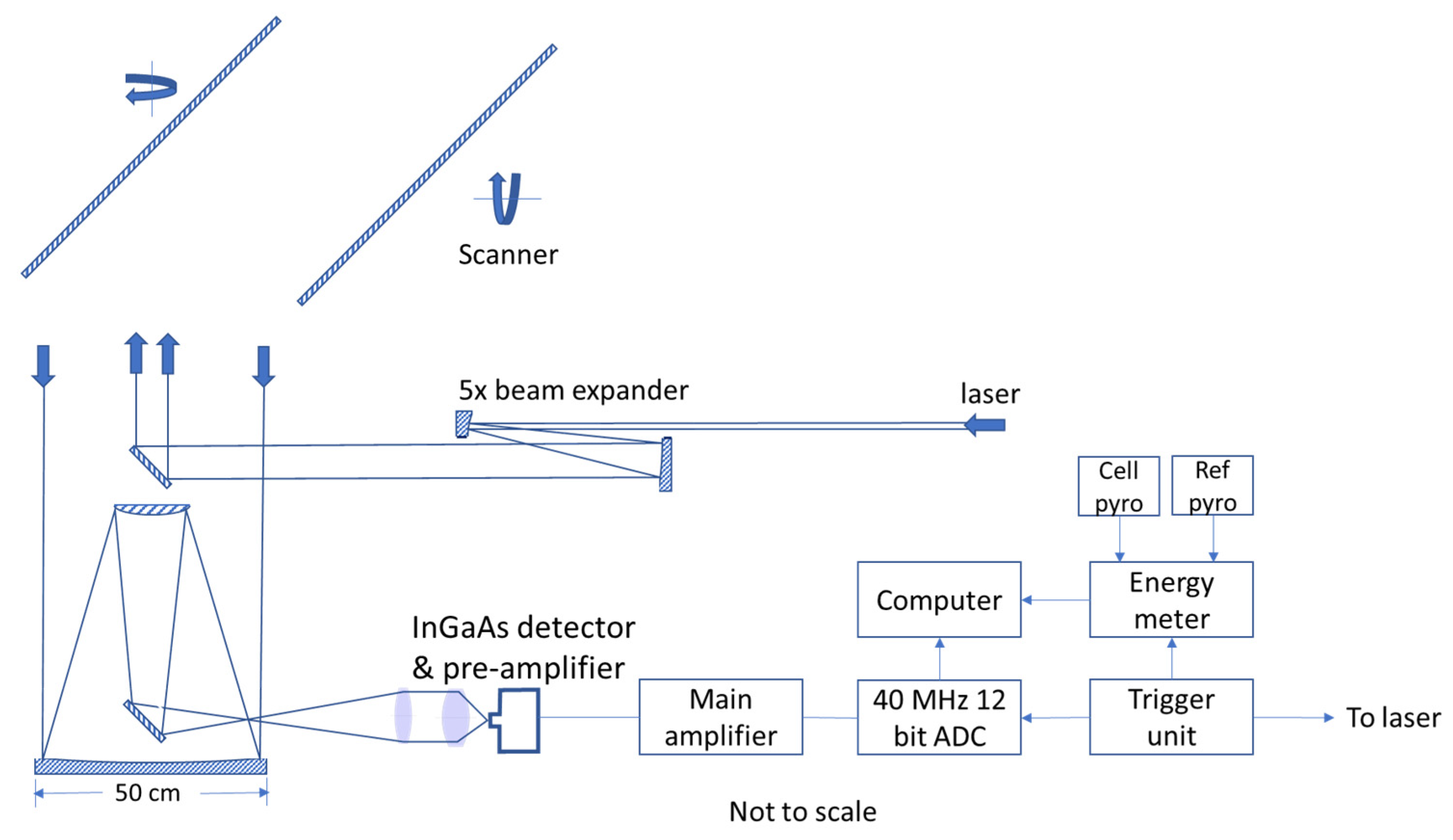
2.1. DIAL System

NPL DIAL system generates IR laser pulses of approximately 9 ns in length at two different wavelengths as previously described in Robinson et al. [17]. As the IR laser pulses pass through the atmosphere a small portion is elastically scattered back, primarily through Mie scattering [29], to the DIAL where they are subsequently detected. The two wavelengths are chosen such that one is absorbed by the species being measured (i.e., the target species) and the other is close in wavelength, therefore experiencing similar scattering, but with minimal absorption by the target species. The range resolved concentration measured along the path of a laser beam can be calculated from the ratio of the two returned signals using the DIAL equation [30,31]. A DIAL scan is made up of different laser path measurements made at various elevations, allowing a 2D concentration measurement plane to be mapped out. Mass emission rates, typically reported in units of either kilograms per hour (kg/h) or tonnes per hour (t/h), are derived by combining the 2D concentration measurement plane with the measured wind vector orthogonal to the concentration plane. The data analysis is done using a proprietary in-house Matlab script (version 1.08). valid emission measurement comprises the mean of a minimum of four scans. Extensive details on the DIAL validation work and application of the methodology including the wind measurements and quality assurance criteria can be find in these publications [16,18,19,28,32]. A schematic of the NPL DIAL’s beam launch optics and detection system is shown in Figure 1.

The choice of wavelengths, laser source and detection system are bespoke for each target species: the details given in the following Section 2.2, Section 2.3 and Section 2.4 are specific for the measurement of CO₂.

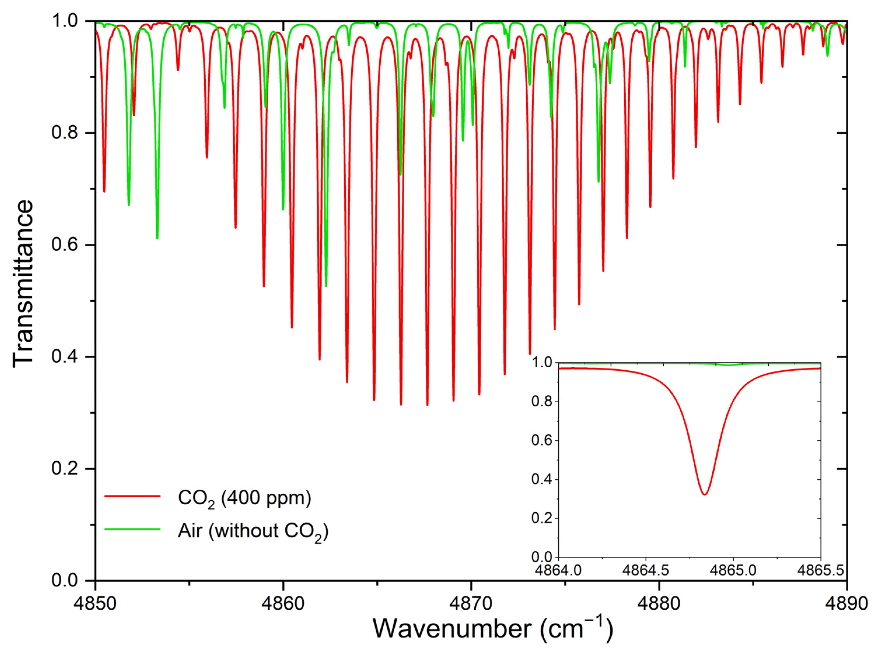
2.2. Wavelength Selection

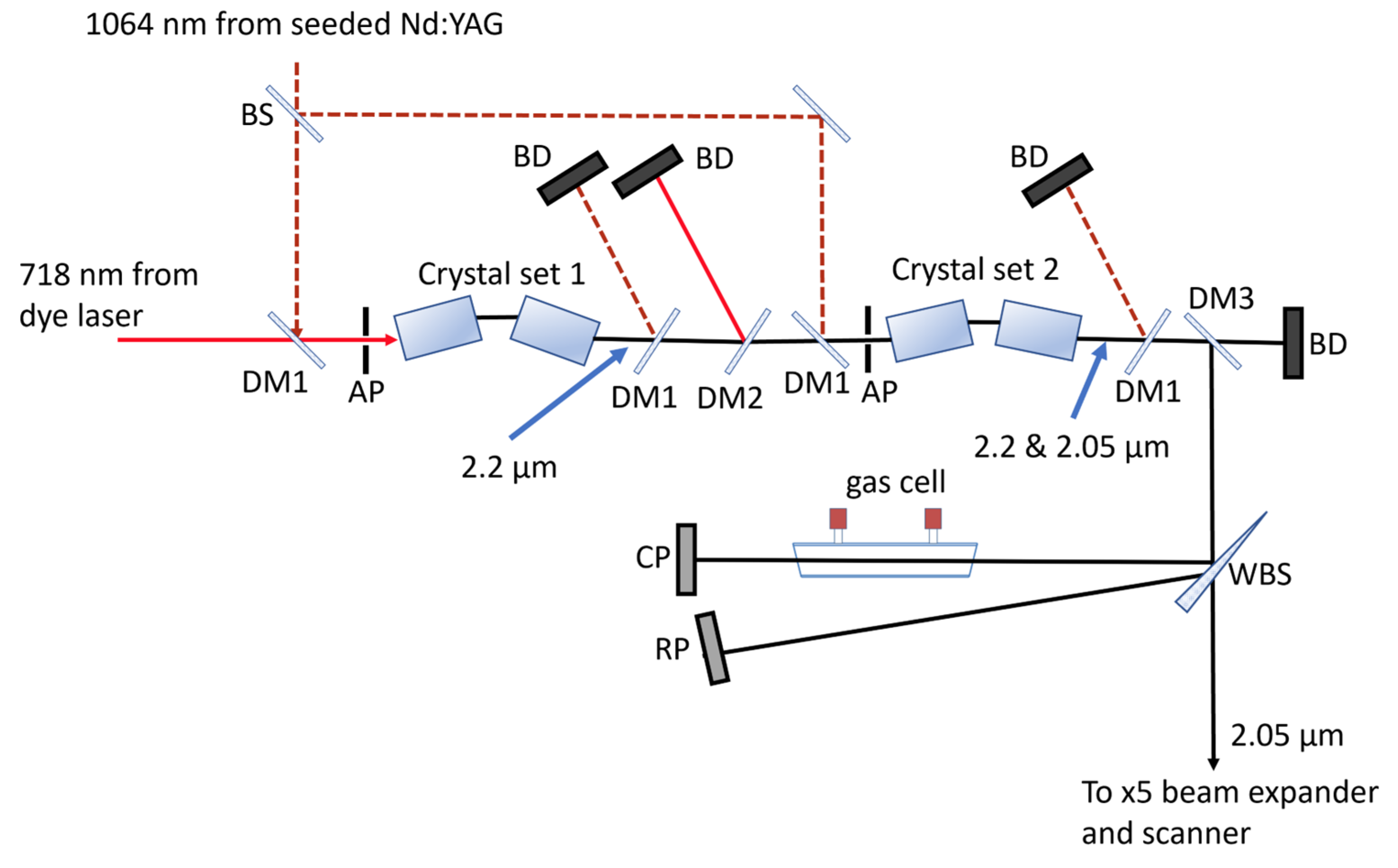
The choice of wavelength determines the DIAL system performance. For example, selecting a wavelength corresponding to a CO₂ absorption peak with a larger absorption coefficient should result in a lower detection limit. However, due to the relatively high background concentration of CO₂ in the atmosphere (~400 ppm) this may result in the laser being entirely absorbed over a short range by the background CO₂. In contrast selecting a weaker absorption peak would make longer range measurements a possibility but at the cost of measurement sensitivity. The previous DIAL CO₂ work used wavelengths around 1.5 µm where absorption is low and this resulted in a high detection limit [21]. This work investigates the use of wavelengths at approximately 2 μm where CO₂ absorption is higher. It should be noted that operating in the 2 µm region will reduce the upper limit for detection, as full absorption of the on-resonant laser energy is more likely to occur. However, the primary focus of this work was to develop a method to measure low level fugitive emissions from CCUS, and weaker absorption lines could be selected if a larger source was being targeted.

Figure 2 depicts a plot of CO₂ transmittance (assuming CO₂ concentration = 400 ppm) calculated using HITRAN on the Web in the 2 μm region with a path length of 1 km (red line) [33]. More specifically, the absorption band shown is the R-branch of a ro–vibrational transition between 4850 and 4890 cm⁻¹. The green line highlights the expected interference due to the absorption from other atmospheric components, primarily water vapour (H₂O), which absorb in this region. Therefore, a careful selection of the on and off resonant wavelengths is required to minimise any interference. One option is the CO₂ absorption peak at 4864.8 cm⁻¹ (2055.58 nm), as H₂O interference is almost negligible between 4864 cm⁻¹ and 4866 cm⁻¹ as shown in the inset of Figure 2. Therefore, the peak at 4864.8 cm⁻¹ was selected as the on-resonant wavelength and 4865.6 cm⁻¹ can be utilized as the off-resonant wavelength. The peaks at 4864.8 cm⁻¹ and 4865.6 cm⁻¹ will henceforth be referred to as the on and the off wavelengths, respectively.

2.3. Laser Source

The laser system uses both the first (1064 nm) and second (532 nm) harmonic frequency outputs of an injection seeded Continuum Powerlite Nd:YAG laser. The 532 nm energy is used as a pump source for a Sirah Cobrastretch dye laser which enables the wavelength fine tuning using a diffraction grating (1800 lines/mm). The laser operates at 10 Hz and the wavelength is switched between the on and off wavelengths on alternative pulses using the rear resonator cavity mirror mounted on a piezoelectric crystal. To generate the 2 µm energy required for this work the dye laser was operated at 718 nm. As shown in Figure 3, a Sirah OPANIR set-up is utilized to generate the 2 µm energy. By using two pairs of Lithium niobate (LiNbO₃) crystals at each stage it is possible to phase match at both the on and off wavelengths. Initially, the output from the dye laser is mixed with a portion of the fundamental 1064 nm laser light from the seeded Nd:YAG laser, via a 8 mm diameter aperture, in the first set of crystals (16 mm × 11 mm × 30 mm) to produce an output at 2.2 µm through difference frequency mixing. Following this, the 2.2 µm beam is further mixed with the remaining 1064 nm light, again via an 8 mm diameter aperture, in the second set of crystals (13 mm × 11 mm × 50 mm) to produce outputs at the desired on and off wavelengths around 2.06 µm. The crystals are angle tuned and held at a fixed temperature in individual ovens. The arrangement used was a result of modifying the existing system which normally operates with output in the 3.3 µm wavelength region. The laser output produced is reported in

Table 1. Laser output parameters.

Parameter	Value	Units
Pulse length	9	ns
Repetition rate	10	Hz
1064 nm Nd:YAG energy	650	mJ
532 nm Nd:YAG energy		mJ
718 nm energy before DFM	50	mJ
1064 nm energy before DFM	60	mJ
2.2 µm energy before OPA	2–5	mJ
1064 nm energy before OPA	200	mJ
2.05 µm output energy	15–20	mJ
On wavelength	2055.58	nm
Off wavelength	2055.24	nm
Divergence	~0.2	mRad

. It should be noted that as both 532 nm and 1064 nm energy is generated simultaneously by the Nd:YAG laser, the time-synchronization of the dye laser pulses and the 1064 nm for the OPANIR stage is maintained by diverting the 1064 nm light through an optical delay line.

Reflections off an uncoated sapphire wedge, sampling the outgoing laser energy, are directed onto pyroelectric laser energy detectors measuring the reference energy and the energy through a 20 cm gas cell containing CO₂ gas of 99.9995% purity at atmospheric pressure. These energy readings are used, when scanning the laser wavelength, to produce absorption spectra and to monitor the absorption ratio of the two wavelengths during measurements to assess and correct for any drift in the wavelengths. It should be noted that any drift in the wavelength increases the absorption ratio. During this study the ratio was relatively stable, for example on Day 2 of the campaign the ratio was observed to vary by approximately ± 0.01, which is equivalent to ~2% variability. A High Finesse WS6 wavemeter continually monitors the dye laser wavelength and is used to independently confirm the correct wavelengths are achieved.

2.4. Detection System

To allow for operation in the 2 µm region, an extended wavelength range InGaAs detector was acquired. The detector head includes the InGaAs photodiode (detector area = 0.196 mm²) and a low noise preamplifier. The main amplifier is linked to the detector head over a 90 cm shielded cable. The detection system at the maximum bandwidth of 13.4 MHz has a specific detectivity of 2.1 × 10¹⁰ cm Hz^1/2/W. Detector signals are then digitised using a Licel 12-bit ADC transient recorder with a sampling rate of 40 Ms/s, which equates to a range resolution of 3.75 m. The unit contains memory so that a sequence of laser shots can be averaged to reduce random noise.

2.5. Calculated Emissions from Test Site

To test the CO₂ DIAL system and measure emissions to the atmosphere under representative conditions, a suitable site with known CO₂ emission sources that could be measured and quantified by a variety of methods (to compare with the DIAL results) was needed. The site selected was a liquefied natural gas (LNG) import terminal which utilizes natural gas-fired heaters to regasify the LNG before input to a grid system. The site has multiple regasification units (RGUs) which vent the combusted fuel products (including CO₂) to atmosphere from stacks. Notably, the amount of gas supplied to the RGUs can be varied to meet network demands.

The CO₂ emissions from the RGUs can be calculated from the amount of gas burned, quality and composition of the gas. Using this information provided by the site’s operator, the CO₂ emission factor for the natural gas combusted can be calculated in tonnes of CO₂ emissions (Q_CO2) per tonne of fuel combusted (Q_fuel), as described in the EU ETS Greenhouse Gas Monitoring and Reporting programme [2]. The net calorific value (net CV expressed in MJ/t_fuel) and the carbon emission factor (CEF, expressed in t_CO2/MJ) of the fuel gas were calculated from the site data provided. Equation (1) shows how these parameters can be multiplied together to provide Q_CO2 expressed in tonnes of CO₂ per hour.

$$Q_{C{O}_2 }=\mathit{CEF} \times net CV\times Q_{fuel}$$

(1)

The operator provided eleven measured quantities to calculate the three parameters in Equation (1). It is not possible to assess the uncertainty for all these variables, consequently it is not possible to provide a full uncertainty assessment of the calculated emissions. Moreover, assumptions have been made regarding the temperature, pressure, and physical properties (i.e., gas compressibility) that can lead to systematic differences for the reported values. Therefore, to ensure an accurate evaluation of the RGU emissions, direct in-stack measurements of the CO₂ emissions were performed by the NPL Industrial Emissions team for comparison to the DIAL measurements and the combustion calculations.

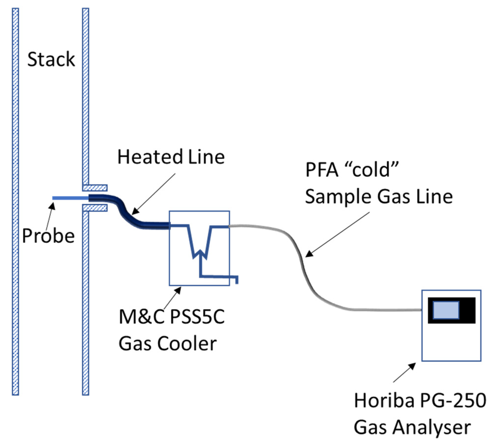
2.6. In-Stack Measurements Methodology

For the in-stack measurements of the CO₂ concentration the requirements of PD CEN/TS 17405:2020 were followed [34]. This specifies the reference method for CO₂ stationary source emission measurements using an infrared spectrometry technique. Measurements were taken using the configuration shown in Figure 4, this included: a portable Horiba PG-250 analyser with an NDIR CO₂ channel (0–20% certified range), a PFA “cold” sample gas line, an M&C PSS5C gas cooler and a heated Environmental Monitoring sampling line (JH3E) and titanium probe. The gas cooler was kept at below 4 °C and the heated sampling line at 180 °C. The flue gas was drawn through the system via the gas cooler internal pump and delivered to the Horiba PG-250.

Prior to the measurements of the stack flow being conducted, measurements of the internal duct area at the measurement plane were made using a stainless-steel measuring rod and a calibrated tape measure. The duct area value has been used to convert the velocity into a volumetric flow rate for each flow test carried out. The location of the measurement points on the measurement plane were determined according to EN 15259:2007 tangential method [34] and the Pitot tube/probe assembly was then marked accordingly. The tangential method is applicable to circular ducts and provides a method and the calculations for dividing the measurement plane in equal areas. Figure 5 shows the stack flow measurement configuration.

The stack gas volumetric flow measurements were conducted in accordance with EN ISO 16911-1:2013 and PD CEN/TR 17078:2017 [36]. These specify manual reference techniques for the determination of flow (EN ISO 16911-1) and provide guidance on how the Standard should be applied and how the QA/QC should be performed (PD CEN/TR 17078). A differential pressure technique based on Pitot tube measurements was used. The measurement system consisted of an S-Type Pitot tube attached to a 1.5 m probe and a Kimo MP210 electronic pressure readout device with a range of 0–2500 Pa. A K-Type thermocouple attached to the Kimo MP210 provided the stack temperature readings.

Before commencing the flow measurements, various pre-test checks were completed in order establish the integrity of the measurement system. These included a visual inspection of the Pitot tube and a leak check of the system which was achieved by using a syringe to pressurise the Pitot tube to 1300 Pa and observing that the reading on the Kimo MP210 remained stable to within 24.5 Pa. A functional check of the Kimo MP210 was also carried out which included checking the zero value of the device and checking that the instrument responded to gas flow. The measurement system was then introduced to the flue gas and a measurement of the gas static pressure was carried out; this was found to be 249 Pa. The static pressure in combination with a measurement of the atmospheric pressure was used to establish the stack gas pressure. A final pretest check consisted of a test at each measurement point for the presence of cyclonic flow (swirl) within the duct which, if significant (cyclonic flow angle >15° of the axial direction), can affect Pitot tube measurements. This was achieved by mounting a digital protractor on the Pitot tube/probe assembly and rotating the assembly so that the planes of the face openings were perpendicular to the stack gas flow and determining the null point (ΔP = 0) by rotating the Pitot tube assembly either clockwise or anticlockwise. At the null point the reading on the protractor corresponds to the degree of swirl of the gas flow in regard to the stack axis at the marked position. The results from these tests highlighted that swirl was detected but all angles were less than 10° so no further action was required.

The flue gas molecular weight was determined by carrying out measurements for oxygen (PG-250 Horiba and associated sampling system) according to EN 14789:2017 [37], carbon monoxide (PG-250 Horiba and associated sampling system) according to EN 15058:2017 [38] and water vapour (calculation method) according to EN 14790:2017 [39].

3. Results

3.1. Derivation of the Differential Absorption Coefficient

Understanding the atmospheric transmittance gives vital information regarding both the range and the sensitivity of the DIAL measurements towards the target species, in this case CO₂. Moreover, in order to correctly assess the concentration of the target species in the atmosphere the differential absorption coefficient Δα has to be derived as accurately as possible. This can be carried out using the following Equations (2) and (3):

$$absorption ratio=\frac{{\left(\raisebox{1ex}{$E_{CP}$}\!\left/ \!\raisebox{-1ex}{$E_{RP}$}\right.\right)}_{on}}{{\left(\raisebox{1ex}{$E_{CP}$}\!\left/ \!\raisebox{-1ex}{$E_{RP}$}\right.\right)}_{off}}=\frac{T_{\mathit{on}}}{T_{\mathit{off}}}=e^{-∆{\alpha }_{cell}\times c\times l}$$

(2)

$$∆\alpha =∆{\alpha }_{cell}\times \frac{{FWHM}_{cell}}{{FWHM}_{atm}}$$

(3)

which use the ratio of the on- and off-resonant cell pyroelectric energy detector (CP) and reference pyroelectric energy detector (RP) energy ratios. This is equivalent to the ratio of the on- and off-wavelength transmittance (T_on and T_off respectively), henceforth known as the absorption ratio. From the absorption ratio is possible to calculate the differential of the on and off resonant absorption coefficients measured in the cell (Δα_cell) as the gas concentration © in the cell and the path length l are known. FWHM_cell and FWHM_atm are the full width at half maximum of the selected absorption peak for the gas cell and atmosphere. The ratio of the two is used to account for the difference between the spectral broadening observed in the cell, where self-broadening of the absorption peak caused by the high purity CO₂ is observed, and the foreign broadening, which occurs in the atmosphere. Only by accounting for these effects the correct absorption coefficient, Δα, can be calculated. Moreover, the absorption coefficient is specific to the system taking into account instrumental factors such as the laser line width.

An average evaluation of Δα_cell was calculated from 19 repeated measurements of a 20 cm gas cell filled with CO₂ (99.9995% purity). It should be noted that the gas cell was refilled four times to reduce systematic bias that could be caused by a poorly filled cell. An average value of Δα_cell = (1.51 ± 0.08) × 10⁻³ ppm⁻¹ km⁻¹ was derived for a differential wavenumber separation of approximately 0.80 cm⁻¹.

From the cell sample data, it was also possible to estimate FWHM_cell = 0.297 cm⁻¹. FWHM_atm was derived experimentally by varying the DIAL’s output wavelength systematically over the range of the absorption peak. At each wavelength the atmospheric CO₂ concentration (calculated from the slope of the path-integrated concentration) was quantified. Figure 6 shows a plot of the wavelength (in wavenumbers) versus the atmospheric CO₂ concentration (ppm) obtained by systematically varying the wavelength of the DIAL output between 4864.25 cm⁻¹ to 4865.25 cm⁻¹ and recording three repeated DIAL measurements of the atmosphere. Each point in Figure 6 is therefore the average of these three datasets, with each set comprising 500 laser shots. It should be noted that a fixed absorption coefficient, calculated at the CO₂ absorption peak wavelength, was used for each datapoint. Consequently, the correct atmospheric CO₂ concentration value is only observed at the CO₂ absorption peak wavelength, which was ~450 ppm. The absorption coefficient in reality is dependent on the wavenumber and, if the correct absorption coefficient was used at any given wavenumber, the plot in Figure 6 would be a ~450 ppm straight line. Given that the aim of the experiment was to estimate the linewidth of the target absorption peak in the atmosphere, a constant absorption coefficient was used.

From the data in Figure 6, it was possible to map out the target absorption peak, and the FWHM_atm was estimated to be 0.239 cm⁻¹. At wavenumbers above 4865 cm⁻¹, the average CO₂ atmospheric concentrations were negative, and a definitive cause of this unexpected result is unknown. Possible explanations for this are either a broadband spectral effect caused in the beam path by the optics or from the co-alignment of the outgoing and incoming optical beam paths. Notably, these explanations would not be relevant to the determination of the linewidth. Another explanation for the observed negative values would be absorption on the off-resonant wavelength caused by either CO₂ or another interfering species, in which case it could be reasonable to remove the negative values from the dataset. However, this is thought to be unlikely as this region of the spectrum was checked carefully in HITRAN (see Figure 2 inset) and, if such interference was present, it could equally affect some of the positive datapoints and the removal of the negative values could introduce a different bias. Moreover, it should be noted that if the negative data were excluded, the derived value of FWHM_atm would only decrease by approximately 4 %. For these reasons, all the data were included in the derivation of FWHM_atm \, as shown in Figure 6. Using this information, the FWHM_cell and FWHM_atm ratio for each cell scans was derived and subsequently a corrected Δα of (1.88 ± 0.14) ×10⁻³ ppm⁻¹ km⁻¹ was calculated. It should be noted that the reported uncertainty is purely statistical and has been expanded to the 95% confidence level.

3.2. DIAL Measurements

The DIAL measurement setup is shown in Figure 7, with the wind data collected from a fixed meteorological mast located approximately 650 m to the northwest of the RGU stack at the position marked as ‘Fixed Mast’. The mast supports four sets of wind sensors at 11.9 m, 9.0 m, 6.2 m and 3.4 m elevations. A 10.5 m wind sensor was also deployed from the DIAL trailer. The wind sensor used to define the wind direction for the emission rate calculation was the top sensor from the fixed mast. The four wind speeds measured at different heights of the fixed mast were used to construct an unperturbed logarithmic vertical wind profile.

During the two-day measurement campaign, the DIAL system was located approximately 130 m from the RGU stack 1. The wind was consistently from a westerly direction and the wind speed was between 2 m/s and 8 m/s. The laser beam line-of-sight (LOS) was downwind of the targeted stack as indicated in Figure 7. The DIAL vertical scans consisted of 11 to 18 lines that captured the CO₂ emission from the targeted plume creating a 2D concentration plane. Each line of the scan consisted of either 150 or 250 laser pulses at each on- and off-wavelength depending on the intensity of the returned signals. For each DIAL scan the CO₂ concentration plane was determined and then combined with the wind vector to calculate the mass emission rate, as described in Section 2.1. All the DIAL scans reported in this work have passed the quality criteria and assurance described in the European Standard EN 17628 [20] and by Innocenti et al. [19].

Figure 8 shows an example plot of the return signals from the received on and off wavelengths scatter from one path measurement of a DIAL scan. This line has passed through the plume of a stack and the off signal shows an enhanced Mie scattering from particles or aerosols in the plume while the on signal shows a decrease where the laser is absorbed by the CO₂ in the plume.

Figure 9 shows the path concentration integrals for two laser paths at different elevations from the same scan. One of the paths shows a steep step increase due the CO₂ absorption in the plume while the other line was above the plume, and it was effectively a measurement of the CO₂ background, which was approximately 600 ppm. This high value can be due to either high CO₂ background concentration from other sources in the industrial area or to the coaxial design of the transmitting and receiving optics that can lead occasionally to range dependent differences in the spatial overlap that, combined with small differences in the alignment of the on- and off-resonant beams, can cause a range-dependent offset and ‘shape’ in the path-concentration integral column, as described in Innocenti et al. (2022) [31]. Either way, the background concentration is subtracted from each path measurement so that only the increased concentration due to the targeted emission plume is used to calculate the 2D concentration plane.

Figure 10 shows a 2D DIAL concentration vertical scan, calculated from 13 path measurement lines, placed over a site map to give a 3D visualization of the plume. The contour plot represents the concentration of the plume above background. The concentration plane is then combined with the horizontal wind vector perpendicular to the measurement plane to determine the mass emission rate.

Each DIAL scan took approximately between 10 and 15 min to complete. During the measurement campaign a total of 28 valid scans of RGU stack 1 were recorded covering four different fuel supply rates. On Day 1 of the campaign seven valid scans were taken during Test 1. The Test 1 measurements period started at approximately 13:15 on Day 1, but the test was halted at 13:40. Measurements were restarted at 15:20 and ran until approximately 16:30, the total test time was approximately 85 min. Tests 2, 3 and 4 took place on Day 2 of the campaign. During Test 2, six scans were recorded between approximately 11:55 and 13:05. Test 3 took place immediately after Test 2 from 13:05 until 14:20, seven scans were recorded in this period. During Test 4, eight scans were recorded between approximately 14:20 and 16:00. The CO₂ mass emission rates are shown in Figure 11 for each scan. The uncertainty of the measurements reported in

Table 2. Comparison of the DIAL, in-stack and combustion calculation results of the CO₂ emitted from RGU stack 1. All values cover the same measurement period and the reported expanded uncertainties provide a 95% level of confidence.

Test	Number of DIAL Scans	DIAL	In-Stack	Calculated	Units
1	7	5.36 ± 1.23	5.29 ± 0.66	5.50	t/h
2	6	6.43 ± 0.53	6.17 ± 0.88	6.21	t/h
3	7	4.51 ± 0.27	4.30 ± 0.78	4.29	t/h
4	8	4.66 ± 0.47	4.58 ± 0.79	4.64	t/h

for each test (supply rate) was estimated based on the standard deviation of the individual emission rate measurements from which each mean emission rate value has been determined. The 95% t-based confidence interval for the mean is reported as the expanded uncertainty as described in EN 17628 [20].

Most of the DIAL scans (28 out of 32) were focused solely on measuring the emissions from RGU stack 1 where the in-stack measurement equipment was set up. The other four DIAL scans were used to measure the emissions from all the other seven RGU stacks in operation, excluding the emissions from RGU stack 1. The CO₂ emission plumes downwind of these seven stacks were clearly visible, as shown in Figure 12. The average emission rate measured from these four scans was 42.2 ± 5.4 t/h with the reported uncertainty expanded to provide a 95% level of confidence. Using the gas usage data and other operational data provided by the operator, it was possible to calculate an emission rate of 40.3 t/h using Equation (1). This value is within the coverage interval of the DIAL measurement and demonstrates that CO₂ emissions from multiple sources could be accurately quantified over a wide range of distances from the DIAL. Furthermore, this demonstrates that substantial emission sources (on the order of 50 t/h) could be measured by DIAL without the whole on-resonant wavelength laser pulse being absorbed by the CO₂ plume and implied that larger sources (>50 t/h) could be measured using this method.

3.3. In-Stack Measurements

At the start of each day of testing, zero grade Nitrogen and a 15.22% (volume fraction) CO₂ span gas (1% relative uncertainty) were supplied to the analyser. The analyser was adjusted both at zero and span. The zero value was checked again after the adjustments. The zero deviation between the adjustment value and the zero check was lower than twice the repeatability at zero therefore satisfying the PD CEN/TS 17405:2020 requirements [34]. The whole measurement system was then leak checked by sealing the probe and measuring the leak flow rate to ensure any potential leak does not exceed 2% of the expected sample gas flow rate. In all tests no identifiable leak was detected. At the end of each day the zero and span gases were re-introduced at the inlet of the analyser to measure the zero and span drift of the analyser. On both days of testing the drift identified was less than 2% of the span value therefore meeting the acceptance criterion of PD CEN/TS 17405:2020. As per the requirements of this standard when drift is less than 2% no correction has been applied to the data; however, the drift was accounted for in the concentration uncertainty calculation.

For the flow measurement, the Pitot tube/probe and thermocouple assembly was then placed at the first marked position, with the impact side of the Pitot tube pointing directly into the gas flow. The temperature and differential pressure were allowed to stabilize, and the differential pressure (ΔP) and temperature was recorded on the appropriate section of an electronic data sheet. The Pitot tube/probe and thermocouple assembly was then moved to the next marked position in the traverse until all measurement points had been measured. Each reading at each point was averaged over at least 1 min. A post-test leak check was carried out at the end of the flow measurements to ensure the integrity of the system had stayed intact. On day 2 due to the weather conditions (high winds) the flow traverse had to be stopped half-way through so only one measurement line out of two was measured. This flow measurement was deemed to be acceptable for the purposes of this study, although it has not been accounted for within the uncertainty budget, so the uncertainty quoted is a best-case scenario.

The mass emission rates were then calculated by multiplying the concentration and flow measurements. The resulting values on a minute-by-minute basis are shown in Figure 13 over the DIAL measuring period of RGU stack 1. The expanded uncertainties reported in Table 2 for each test were calculated by propagating in quadrature the flow and concentration uncertainty budgets. The variability of the concentration measurement over each test period was also considered; however, it did not have any effect as it was more than one order of magnitude lower than the concentration measurement uncertainty.

3.4. Calculated Emissions

The site’s operator provided the amount of gas supplied to the RGU stack 1 on a minute-by-minute basis and other operational data, from which it was possible to estimate the CO₂ emissions using Equation (1). Figure 14 shows the calculated emission rates over the DIAL measuring period of RGU stack 1.

Table 2 reports the average calculated emission for each test with different fuel supply rates. Unfortunately, as mentioned in Section 2.5, it was not possible to assess the uncertainty for these calculations.

3.5. Comparison of Results

During the measurement campaign four different fuel rates were supplied to RGU stack 1. The DIAL, in-stack and combustion calculation results are compared in Table 2 and Figure 15 for each test.

From Table 2 it can be seen that the DIAL results compare very well with both the in-stack and calculated CO₂ emissions as all the values for each test fall within the coverage interval of the reported DIAL data. This is highlighted further in Figure 15 where the DIAL quantified emission rates are plotted against the in-stack measurements. A Deming regression, which considers uncertainty in both x- and y data values, was performed using R; this yielded a linear regression of y (t/h) = (1.04 ± 0.21) x − (0.02 ± 1.00), the standard errors in the gradient and y-intercept from this fitting have also been reported [40,41,42]. Notably, the standard error in both the gradient and y-intercept are significant and likely exacerbated by the limited dataset, the small dynamic range of the emission rates and the magnitude of the associated uncertainty of the in-stack measurements. However, the gradient of the fitting is close and 1 and the y-intercept is near zero, which suggests that any bias in the DIAL data is likely small. These results demonstrates that the 2 µm DIAL CO₂ configuration described in this work is a viable method for quantifying CO₂ emissions in the observed range.

The DIAL uncertainty for Test 1 during Day 1 is significantly higher than the uncertainty reported for the other 3 tests on Day 2. Notably, on the morning of the second day the pointing of the transmitting optical path was adjusted to increase the signal returns in the far field, leading to an improved optical alignment, which significantly increased the signal received. Therefore, it is believed that the system configuration had not been fully optimized during Test 1. This is reflected in the lower uncertainties observed during Tests 2, 3 and 4 measurements. It is therefore important that these tests with lower DIAL uncertainty still compare well with the in-stack measurements and calculated CO₂ emissions.

As noted in Section 3.3, the in-stack flow measurement taken during Tests 2, 3 and 4 are the best cases scenarios and could have a higher associated uncertainty. However, this does not affect the conclusions from this work as all the results compare well within the boundaries of the reported uncertainties.

Robinson et al. estimated a detection limit of approximately 260 t/h was for CO₂ emission quantification in the 1.5 µm wavelength region using NPL’s previous DIAL system [21]. This value was estimated using the definition of detection limit from the European standard for instrument type testing, EN 15267-3, which is twice the standard deviation at zero [43]. In this study no distinct measurements of the background CO₂ levels were made using the DIAL system. However, it was possible to analyse a region further downwind of the RGU stack 1, where no emissions were observed nor expected, and from this to estimate the detection limit for the given measurement. In order to calculate a detection limit as representative as possible of the measured plume, a region approximately the same size as the plume was analysed between 180 m and 200 m from the DIAL on the lines where the CO₂ plume was observed. This was carried out on the DIAL scans taken during Test 2 resulting in an average emission rate of 0.01 t/h and a standard deviation of 0.06 t/h. Using the definition outlined in EN 15267-3 a detection limit of 0.12 t/h was estimated for this data, more than three orders of magnitude lower than observed in the 1.5 µm wavelength region. However, it is acknowledged that the observed difference in detection limit is not only due to the wavelength region selected and that other factors may also impact it. For example, factors such as the output laser energy and atmospheric scattering conditions were different between these two studies.

It should also be noted that the signal-to-noise in the analysed region for the detection limit data was lower than in the region where the plume was located. Moreover, as this region is further away from the DIAL, the distance between scan lines is greater and hence the overall area analysed is larger than that of the plume. Therefore, the detection limit derived is likely to be an overestimate of the detection limit for the measured plume. To determine the detection limit for CO₂ DIAL measurements, an uncertainty assessment should be carried as previously demonstrated in Innocenti et al. using a different detection system for species measured at 3.3 µm [29].

4. Discussion

In this paper we have successfully demonstrated the use of DIAL for remote measurement of CO₂ emissions at a wavelength of about 2 µm with a significant improvement when compared to the results previously obtained at 1.5 µm. The results from the intercomparison with in-stack measurements at an LNG import terminal indicate that the DIAL can be used to accurately quantify CO₂ emissions from industrial sources.

As part of this study, a system specific differential absorption coefficient was derived using data collected from measurements of 20 cm gas cells containing pure (99.9995%) CO₂. The derived differential absorption coefficient was corrected for any self-broadening of the absorption peak, leading to a value of Δα = (1.88 ± 0.14) × 10⁻³ ppm⁻¹ km⁻¹. It should be noted only a relatively small number of gas cell measurements were used for this calculation and that the FWHM_atm was measured only once. In the future, the measurement of the FWHM_atm should be reproduced to assess the repeatability and uncertainty of the results. Furthermore, measurements of the gas cells will continue to be collected during future CO₂ DIAL work, incorporating these data into the calculation of Δα would further reduce its associated uncertainty and any bias caused by the current sample size. Nonetheless, this improvement is expected to be small given that the intercomparison of the DIAL data with the in-stack and calculated results does not suggest any systematic discrepancy that could be caused by the current estimation of Δα. On the other hand, the lack of knowledge of any systematic uncertainty from the calculated emissions and the relatively large uncertainty from the in-stack measurements, when compared to known sources, make it difficult to assess any small systematic uncertainty in the DIAL measurements.

The LNG import terminal had multiple RGUs in operation and the DIAL quantified the emissions in a single measurement plane from seven RGUs stacks up to a range of 350 m from the DIAL. This is important as it shows that emissions up to 50 t/h could easily be measured by DIAL. However, it is difficult to assess the actual maximum emission rate that the DIAL could measure at these wavelengths as this depends not only by the absorption strength but also on other factors such as the overall return signal strength, the distance of the plume from the DIAL, the overall extension of the plume and the wind speed.

The next steps in the development of the DIAL CO₂ capability is to continue the validation process using a set-up such as NPL’s controlled release facility [32] to demonstrate quantification of smaller sources and obtain a better understanding of the detection limit of quantification for CO₂ measurements. This type of test would also help to assess any potential systematic uncertainty due to Δα. Conversely, to evaluate the maximum detectable emission rate, a similar study should be repeated in the future at facilities with higher CO₂ emission rates such as a power station. It would also be valuable to trial the CO₂ DIAL at a CCUS facility as this would help to demonstrate the potential of the technique for measuring fugitive CO₂ emissions. Lastly, a full analysis of the CO₂ DIAL uncertainty should be performed as previously demonstrated in Innocenti et al. for the species measured in the 3.3 µm wavelength region [31].

References

1. Intergovernmental Panel on Climate Change. Climate Change 2021–The Physical Science Basis: Working Group I Contribution to the Sixth Assessment Report of the Intergovernmental Panel on Climate Change, 1st ed.; Cambridge University Press: Cambridge, UK, 2023. [Google Scholar] [CrossRef]
2. 32018R2066; Commission Implementing Regulation (EU) 2018/2066 on the Monitoring and Reporting of Greenhouse Gas Emissions Pursuant to Directive 2003/87/EC of the European Parliament and of the Council and Amending Commission Regulation (EU) No 601/2012. European Commission: Brussels, Belgium, 2018.
3. Timonen, K.; Sinkko, T.; Luostarinen, S.; Tampio, E.; Joensuu, K. LCA of anaerobic digestion: Emission allocation for energy and digestate. J. Clean. Prod. 2019, 235, 1567–1579. [Google Scholar] [CrossRef]
4. Gardner, N.; Manley, B.J.W.; Pearson, J.M. Gas emissions from landfills and their contributions to global warming. Appl. Energy 1993, 44, 165–174. [Google Scholar] [CrossRef]
5. Gueddari-Aourir, A.; García-Alaminos, A.; García-Yuste, S.; Alonso-Moreno, C.; Canales-Vázquez, J.; Zafrilla, J.E. The carbon footprint balance of a real-case wine fermentation CO2 capture and utilization strategy. Renew. Sustain. Energy Rev. 2022, 157, 112058. [Google Scholar] [CrossRef]
6. UK Government. Net Zero Strategy: Build Back Greener; UK Government: London, UK, 2021.
7. McGonigle, A.J.S. Volcano remote sensing with ground-based spectroscopy. Phil. Trans. R. Soc. A Math. Phys. Eng. Sci. 2005, 363, 2915–2929. [Google Scholar] [CrossRef]
8. Bailey, D.M.; Adkins, E.M.; Miller, J.H. An open-path tunable diode laser absorption spectrometer for detection of carbon dioxide at the Bonanza Creek Long-Term Ecological Research Site near Fairbanks, Alaska. Appl. Phys. B 2017, 123, 245. [Google Scholar] [CrossRef]
9. Xin, F.; Li, J.; Guo, J.; Yang, D.; Wang, Y.; Tang, Q.; Liu, Z. Measurement of Atmospheric CO2 Column Concentrations Based on Open-Path TDLAS. Sensors 2021, 21, 1722. [Google Scholar] [CrossRef]
10. Lan, L.; Ghasemifard, H.; Yuan, Y.; Hachinger, S.; Zhao, X.; Bhattacharjee, S.; Bi, X.; Bai, Y.; Menzel, A.; Chen, J. Assessment of Urban CO2 Measurement and Source Attribution in Munich Based on TDLAS-WMS and Trajectory Analysis. Atmosphere 2020, 11, 58. [Google Scholar] [CrossRef]
11. Nwaboh, J.A.; Werhahn, O.; Ortwein, P.; Schiel, D.; Ebert, V. Laser-spectrometric gas analysis: CO2–TDLAS at 2 µm. Meas. Sci. Technol. 2013, 24, 015202. [Google Scholar] [CrossRef]
12. Hrad, M.; Huber-Humer, M.; Reinelt, T.; Spangl, B.; Flandorfer, C.; Innocenti, F.; Yngvesson, J.; Fredenslund, A.; Scheutz, C. Determination of methane emissions from biogas plants, using different quantification methods. Agric. For. Meteorol. 2022, 326, 109179. [Google Scholar] [CrossRef]
13. Crisp, D. NASA Orbiting Carbon Observatory: Measuring the column averaged carbon dioxide mole fraction from space. J. Appl. Remote Sens. 2008, 2, 023508. [Google Scholar] [CrossRef]
14. Hakkarainen, J.; Ialongo, I.; Tamminen, J. Direct space-based observations of anthropogenic CO2 emission areas from OCO-2. Geophys. Res. Lett. 2016, 43, 11400–11406. [Google Scholar] [CrossRef]
15. Suto, H.; Kataoka, F.; Kikuchi, N.; Knuteson, R.O.; Butz, A.; Haun, M.; Buijs, H.; Shiomi, K.; Imai, H.; Kuze, A. Thermal and near-infrared sensor for carbon observation Fourier transform spectrometer-2 (TANSO-FTS-2) on the Greenhouse gases Observing SATellite-2 (GOSAT-2) during its first year in orbit. Atmos. Meas. Tech. 2021, 14, 2013–2039. [Google Scholar] [CrossRef]
16. Pultarova, T. New Satellite to Police Carbon Dioxide Emitters from Space. Available online: https://www.space.com/ghgsat-carbon-dioxide-detecting-satellite-to-launch (accessed on 8 February 2023).
17. Robinson, R.; Gardiner, T.; Innocenti, F.; Woods, P.; Coleman, M. Infrared differential absorption Lidar (DIAL) measurements of hydrocarbon emissions. J. Environ. Monit. 2011, 13, 2213–2220. [Google Scholar] [CrossRef] [PubMed]
18. Innocenti, F.; Robinson, R.A.; Gardiner, T.D.; Tompkins, J.; Smith, S.; Lowry, D.; Fisher, R. Measurements of Methane Emissions and Surface Methane Oxidation at Landfills, WR1125; Report prepared for Defra by NPL; Defra: London, UK, 2013; p. 89.
19. Innocenti, F.; Robinson, R.; Gardiner, T.; Howes, N.; Yarrow, N. Comparative Assessment of Methane Emissions from Onshore LNG Facilities Measured Using Differential Absorption Lidar. Environ. Sci. Technol. 2023, 57, 3301–3310. [Google Scholar] [CrossRef] [PubMed]
20. CEN EN 17628; Fugitive and Diffuse Emissions of Common Concern to Industry Sectors Standard Method to Determine Diffuse Emissions of Volatile Organic Compounds into the Atmosphere. 2022. Available online: https://standards.cencenelec.eu/dyn/www/f?p=205:110:0::::FSP_PROJECT,FSP_LANG_ID:67021,25&cs=1499A1C530EC17BFF9D3EB0305EFECA18 (accessed on 2 August 2023).
21. Robinson, R.A.; Gardiner, T.D.; Innocenti, F.; Finlayson, A.; Woods, P.T.; Few, J.F.M. First measurements of a carbon dioxide plume from an industrial source using a ground based mobile differential absorption lidar. Environ. Sci. Process. Impacts 2014, 16, 1957–1966. [Google Scholar] [CrossRef]
22. Stroud, J.R.; Dienstfrey, W.J.; Plusquellic, D.F. Study on Local Power Plant Emissions Using Multi-Frequency Differential Absorption LIDAR and Real-Time Plume Tracking. Remote Sens. 2023, 15, 4283. [Google Scholar] [CrossRef]
23. Yue, B.; Yu, S.; Li, M.; Wei, T.; Yuan, J.; Zhang, Z.; Dong, J.; Jiang, Y.; Yang, Y.; Gao, Z.; et al. Local-Scale Horizontal CO2 Flux Estimation Incorporating Differential Absorption Lidar and Coherent Doppler Wind Lidar. Remote Sens. 2022, 14, 5150. [Google Scholar] [CrossRef]
24. Ismail, S.; Koch, G.; Abedin, N.; Refaat, T.; Rubio, M.; Singh, U. Development of Laser, Detector, and Receiver Systems for an Atmospheric CO2 Lidar Profiling System. In Proceedings of the 2008 IEEE Aerospace Conference, Big Sky, MT, USA, 1–8 March 2008; pp. 1–7. [Google Scholar]
25. Refaat, T.F.; Ismail, S.; Koch, G.J.; Rubio, M.; Mack, T.L.; Notari, A.; Collins, J.E.; Lewis, J.; De Young, R.; Choi, Y.; et al. Backscatter 2-μm Lidar Validation for Atmospheric CO2 Differential Absorption Lidar Applications. IEEE Trans. Geosci. Remote Sens. 2011, 49, 572–580. [Google Scholar] [CrossRef]
26. Singh, U.N.; Refaat, T.F.; Petros, M. Triple-pulse integrated path differential absorption lidar for carbon dioxide measurement—Novel lidar technologies and techniques with path to space. In Proceedings of the 2017 IEEE International Geoscience and Remote Sensing Symposium (IGARSS), Fort Worth, TX, USA, 23–28 July 2017; pp. 4212–4215. [Google Scholar]
27. Gibert, F.; Flamant, P.H.; Cuesta, J.; Bruneau, D. Vertical 2-μm Heterodyne Differential Absorption Lidar Measurements of Mean CO2 Mixing Ratio in the Troposphere. J. Atmos. Ocean. Technol. 2008, 25, 1477–1497. [Google Scholar] [CrossRef]
28. Gibert, F.; Edouart, D.; Cénac, C.; Pellegrino, J.; Le Mounier, F.; Dumas, A. 2-μm Coherent DIAL for CO2, H2O and Wind Field Profiling in the Lower Atmosphere: Instrumentation and Results. EPJ Web Conf. 2016, 119, 03005. [Google Scholar] [CrossRef]
29. Bohren, C.F.; Huffman, D.R. Absorption and Scattering of Light by Small Particles; Wiley-VCH: Weinheim, Germany, 2004; ISBN 978-0-471-29340-8. [Google Scholar]
30. Measures, R.M. Laser Remote Sensing: Fundamentals and Applications; Wiley: New York, NY, USA, 1984; ISBN 978-0-471-08193-7. [Google Scholar]
31. Innocenti, F.; Gardiner, T.; Robinson, R. Uncertainty Assessment of Differential Absorption Lidar Measurements of Industrial Emissions Concentrations. Remote Sens. 2022, 14, 4291. [Google Scholar] [CrossRef]
32. Gardiner, T.; Helmore, J.; Innocenti, F.; Robinson, R. Field Validation of Remote Sensing Methane Emission Measurements. Remote Sens. 2017, 9, 956. [Google Scholar] [CrossRef]
33. HITRAN on the Web. Available online: https://hitran.iao.ru/ (accessed on 8 August 2022).
34. CEN/TS 17405:2020; Stationary Source Emissions-Determination of the Volume Concentration of Carbon Dioxide-Reference Method: Infrared Spectrometry. Available online: https://standards.cencenelec.eu/dyn/www/f?p=CEN:110:0::::FSP_PROJECT,FSP_ORG_ID:66891,6245&cs=1DEC7E3239BF18057FA7D1E7B51D5CDAF (accessed on 2 August 2023).
35. EN 15259:2007; Air Quality-Measurement of Stationary Source Emissions-Requirements for Measurement Sections and Sites and for the Measurement Objective, Plan and Report. 2007. Available online: https://standards.cencenelec.eu/dyn/www/f?p=CEN:110:0::::FSP_PROJECT,FSP_ORG_ID:22623,6245&cs=1ED53AEC54D26A0BC2E5A772A04F4BCDB (accessed on 2 August 2023).
36. CEN/TR 17078:2017; Stationary Source Emissions-Guidance on the Application of EN ISO 16911-1. 2017. Available online: https://standards.cencenelec.eu/dyn/www/f?p=CEN:110:0::::FSP_PROJECT,FSP_ORG_ID:62770,6245&cs=160F34108A1ECA2689CAEA5977FCC0502 (accessed on 2 August 2023).
37. EN 14789:2017; Stationary Source Emissions—Determination of Volume Concentration of Oxygen—Standard Reference Method: Paramagnetism. 2017. Available online: https://www.en-standard.eu/csn-en-14789-stationary-source-emissions-determination-of-volume-concentration-of-oxygen-standard-reference-method-paramagnetism/ (accessed on 2 August 2023).
38. EN 15058:2017; Stationary Source Emissions-Determination of the Mass Concentration of Carbon Monoxide-Standard Reference Method: Non-Dispersive Infrared Spectrometry. 2017. Available online: https://standards.cencenelec.eu/dyn/www/f?p=CEN:110:0::::FSP_PROJECT,FSP_ORG_ID:39063,6245&cs=15C8FC63EC8538A17755FCE8DD923D00E (accessed on 2 August 2023).
39. EN 14790:2017; Stationary Source Emissions-Determination of the Water Vapour in Ducts-Standard Reference Method. 2017. Available online: https://standards.cencenelec.eu/dyn/www/f?p=CEN:110:0::::FSP_PROJECT,FSP_ORG_ID:39062,6245&cs=1AD65D866611A52E23DA09770A16F2315 (accessed on 2 August 2023).
40. Therneau, T. Deming: Deming, Thiel-Sen and Passing-Bablock Regression. R Package Version 1.0-1 2014. Available online: https://cran.r-project.org/web/packages/deming/vignettes/deming.pdf (accessed on 30 July 2023).
41. Deming, W.E. Statistical Adjustment of Data; Unabridged and Corr. Republication; Dover Publications: New York, NY, USA, 1964. [Google Scholar]
42. Fasano, G.; Vio, R. Fitting a Straight Line with Errors on both Coordinates. Bull. D’information Du Cent. De Donnees Stellaires 1988, 35, 191. [Google Scholar]
43. EN 15267-3:2007; Air Quality-Certification of Automated Measuring Systems-Part 3: Performance Criteria and Test Procedures for Automated Measuring Systems for Monitoring Emissions from Stationary Sources. 2007. Available online: https://standards.cencenelec.eu/dyn/www/f?p=CEN:110:0::::FSP_PROJECT,FSP_ORG_ID:22226,6245&cs=17DC65A9B48218CF7878CAF72B4F06830 (accessed on 15 September 2023).
Figure 1. Schematic of the NPL DIAL facility’s beam launch optics and detection system.
Remotesensing 15 05403 g001
Figure 2. Plot of HITRAN modelled data of the absorption for CO2 in the atmosphere for a path length of 1 km. The red line represents the transmittance of the CO2 (400 ppm equivalent) between 4850–4890 cm−1. The green line shows possible interference from other molecules in the air (water mixing ratio = 1.5%). (Inset) A plot of the same HITRAN model centred on the selected on-resonant CO2 absorption peak at 4864.8 cm−1 (the target peak).
Remotesensing 15 05403 g002
Figure 3. Laser Diagram, BS—Beam Splitter, BD—Beam Dump, DM1—Dichroic Mirror high reflectance (HR) 1064 nm, DM2—Dichroic Mirror HR 718 nm, DM3—Dichroic Mirror HR 2.05 µm, AP—8 mm diameter aperture, Crystal set 1 and 2—LiNbO3 type 1, WBS—Wedged Beam Splitter, CP—Cell pyroelectric energy detector, RP—Reference pyroelectric energy detector, gas cell—20 cm long filled with 100% CO2.
Remotesensing 15 05403 g003
Figure 4. Arrangement of equipment for in-stack measurements.
Remotesensing 15 05403 g004
Figure 5. Stack flow measurement configuration. The numbers shown highlight the different measurement locations used as part of the tangential method. These locations are selected at specific points to split the duct into equal areas [35].
Remotesensing 15 05403 g005
Figure 6. A plot of the CO2 concentration in the atmosphere versus DIAL output wavelength. Each datapoint is calculated using a constant absorption coefficient which was measured at the CO2 absorption peak wavelength. The error bars shown represent the observed standard deviation from the measurement. The red line is the optimal unweighted fitting through the experimentally measured data using a Voigt function.
Remotesensing 15 05403 g006
Figure 7. Measurement configuration for a single stack.
Remotesensing 15 05403 g007
Figure 8. An example of the on and off return signals from an average of 150 on wavelength pulses and 150 off wavelength pulses.
Remotesensing 15 05403 g008
Figure 9. Example of path concentration integrals for two laser paths at different elevations. The purple line shows a laser path measurement that passes through the plume while the orange line shows a lase path above the plume representing a measurement of the CO2 background. Note: the data below <80 m are not plotted as the return signals typically starts after 50 m due to the telescope configuration.
Remotesensing 15 05403 g009
Figure 10. Three-dimensional representation of the measured [CO2 concentration above background from the RGU stack 1. The black markers along the LOS are at 100 m intervals. (DIAL not to scale).
Remotesensing 15 05403 g010
Figure 11. Plot of the 28 scans measuring the emission from RGU stack 1. The time given in parenthesis relates to the duration of each test.
Remotesensing 15 05403 g011
Figure 12. Three-dimensional representation of the measured CO2 concentration above background from 7 RGU stacks. The black markers on the LOS are at 100 m intervals. (DIAL not to scale).
Remotesensing 15 05403 g012
Figure 13. Timeseries of the in-stack measurement of RGU stack 1 over the DIAL measuring period.
Remotesensing 15 05403 g013
Figure 14. Timeseries of the calculated emission rates of RGU stack 1 over the DIAL measuring period.
Remotesensing 15 05403 g014
Figure 15. Plot of the DIAL CO2 emission rates measured for the various tests versus the in-stack CO2 rates measured from RGU stack 1. The error bars are equivalent to the standard (not expanded) uncertainties from the measurements. The dashed green line is equal to the line y = x. The solid red line is a regression fitting which considers the uncertainty of both x and y values.
Remotesensing 15 05403 g015