Applications of Deep Learning-Based Super-Resolution Networks for AMSR2 Arctic Sea Ice Images

Abstract

Studies have indicated that the decrease in the extent of Arctic sea ice in recent years has had a significant impact on the Arctic ecosystem and global climate. In order to understand the evolution of sea ice, it is becoming increasingly imperative to have continuous observations of Arctic-wide sea ice with high spatial resolution. Passive microwave sensors have the benefit of being less susceptible to weather, wider coverage, and higher temporal resolution. However, it is challenging to retrieve accurate parameters of sea ice due to the low spatial resolution of passive microwave images. Therefore, improving the spatial resolution of passive microwave images is beneficial for reducing the uncertainty of sea ice parameters. In this paper, four competitive multi-image super-resolution (MISR) networks are selected to explore the applicability of the networks on multi-frequency Advanced Microwave Scanning Radiometer 2 (AMSR2) images of Arctic sea ice. The upsampling factor is set to 4 in the experiment. Firstly, the optimal input lengths of the image sequence for the four MISR networks are found, and then the best network on different frequency band images is further identified. Furthermore, some factors, including seasons, sea ice motion, and polarization mode of images, that may affect the super-resolution (SR) results are analyzed. The experimental results indicate that utilizing images from winter yields superior SR results. Conversely, SR results are the worst during summer across all four MISR networks, exhibiting the largest difference in PSNR of 4.48 dB. Additionally, the SR performance is observed to be better for images with smaller magnitudes of sea ice motion compared to those with larger motions, with the maximum PSNR difference of 2.04 dB. Finally, the SR results for vertically polarized images surpass those for horizontally polarized images, showcasing an average advantage of 4.02 dB in PSNR and 0.0061 in SSIM. In summary, valuable suggestions for selecting MISR models for passive microwave images of Arctic sea ice at different frequency bands are offered in this paper. Additionally, the quantification of the various impact factors on SR performance is also discussed in this paper, which provides insights into optimizing MISR algorithms for passive microwave sea ice imagery.

1. Introduction

Arctic sea ice plays a critical role in stabilizing the global climate by regulating atmospheric circulation, ocean circulation, etc. [1,2,3]. Because of its high reflectivity, sea ice reflects most of the solar radiation, which is beneficial to cooling the Arctic region and regulating the exchange of heat and moisture between the atmosphere and ocean in the Arctic [4,5,6]. In recent years, there has been a significant decrease in the Arctic sea ice extent [1,7,8,9], causing decreases in the albedo of the Arctic region, which in turn accelerates Arctic warming [4]. The reduction of sea ice also threatens Arctic marine mammal species that depend on sea ice for prey and survival [10,11]. Additionally, it also leads to an increased navigation requirement for Arctic shipping and other maritime activities through the Northern Sea Route [12]. Therefore, it is crucial to observe the key parameters of Arctic sea ice, such as sea ice concentration (SIC), accurately, which is conducive to providing sea ice observations for Arctic ecosystem balance studies, global climate change research, and Arctic route design [10,11,12,13].

Traditional monitoring of Arctic sea ice has relied on in situ observations from Arctic scientific expeditions, which are influenced by harsh weather conditions and limited in the context of investigation. Fortunately, remote sensing is an effective means of monitoring Arctic sea ice on a large scale. Passive microwave images have large advantages for the observations of Arctic sea ice since they are not affected by weather and have broad spatial coverage and high temporal resolution [14,15]. Since 1978, they have been providing continuous observation missions of the Arctic region for more than 40 years, including Scanning Multichannel Microwave Radiometer (SMMR) (1978–1987), the Special Sensor Microwave Imager (SSM/I) (1987–2008), Special Sensor Microwave Imager Sounder (SSMIS) (2003–present), the Advanced Microwave Scanning Radiometer for the earth observing system (AMSR-E) (2002–2011), and the Advanced Microwave Scanning Radiometer 2 (AMSR2) (2012–present) [16]. However, the spatial resolution of passive microwave images is much lower than that of optical and Synthetic Aperture Radar (SAR) images. At present, the highest spatial resolution that can be achieved by passive microwave data is obtained by AMSR2 at 89 GHz, with a footprint of 5 × 3 km and a sampling interval of 5 km, but it is still not sufficient for high-resolution parameter inversion of Arctic sea ice. For example, the average width of leads in the central Arctic region is approximately 2–4 km [17], while the commonly used highest gridded spatial resolution of the AMSR2 SIC product at 89 GHz is 6.25 km from the University of Bremen [18], which is difficult to identify such narrow leads, affecting the accuracy of turbulent exchange analysis between the ocean and atmosphere [19]. Another example is that the average Arctic sea ice motion speed is approximately 4 cm/s (3.5 km/day) [20], and the highest resolution of the daily sea ice motion product based on passive microwave image is 12.5 km [21], which cannot recognize small magnitudes of sea ice motion, thus preventing further understanding of the sea ice’s response to the environment in the arctic region [20]. Therefore, improving the spatial resolution of passive microwave images is significant for high spatiotemporal resolution parameter inversion of Arctic sea ice.

Traditional methods to improve the spatial resolution of passive microwave images include using linear combinations of brightness temperature data in the overlapping region of footprints depending on the antenna pattern of the radiometer, such as the Backus–Gilbert (BG) method [22,23], where the accurate prior knowledge is very important for the reliability of resolution enhancement. Recently, image super resolution (SR) methods based on machine learning and deep learning have shown great potential for improving the spatial resolution of remote sensing images [14,24,25,26]. Xian et al. (2017) and Petrou et al. (2018) improve the spatial resolution of passive microwave images using the machine learning approach based on Gaussian Mixture Models (GMM), which relies on learning multiple regression models between the LR image and HR image from image dataset [14,27]. Moreover, some single-image super-resolution (SISR) techniques based on convolutional neural networks are proposed to enhance the spatial resolution of images from the FY-3C microwave radiometer imager (MWRI) [28,29,30,31]. Compared to SISR methods, multi-image super-resolution (MISR) methods can use temporal-spatial complementary information between sequence images to reconstruct the target image to be resolved, reducing the artifacts and the influence of noise and generating finer textures and sharper edges [32]. Salvetti et al. (2020) and Arefin et al. (2020) use deep learning-based MISR methods to enhance the resolution of optical remote sensing images [33,34]. Liu et al. (2022) propose an MISR network for passive microwave images and validate the effectiveness of the network in the 89 GHz band [15]. Although there are few MISR networks designed for multi-frequency bands passive microwave images, current state-of-the-art MISR networks for natural images have the potential to be used as a reference framework for passive microwave images in the Arctic region. Compared to natural images, passive microwave remote sensing images have a lower spatial resolution, with unclear boundaries of objects and insufficient texture information, making it difficult to extract image features. Some passive microwave images in specific frequency bands may also be influenced by environmental factors. For example, the AMSR2 passive microwave image at 89 GHz is sensitive to water vapor and other factors in the Arctic atmosphere, which makes it difficult to provide accurate feature information. Additionally, both thermodynamic (i.e., melting and freezing) and dynamic (i.e., rotation, break-up, and aggregation) processes accompany the motion of sea ice, resulting in the morphology changes of sea ice [15]. This will make the identification and tracking of the same piece of sea ice in sequence images more challenging. What is more, the magnitude of sea ice motion shows large differences within adjacent areas due to several factors, such as ocean currents, temperature, and surface wind speed, making it difficult to choose a uniform spatial scale at which to track sea ice in sequence images. In areas where the magnitude of sea ice motion is large, it can even result in a few image features in the previous image succeeding to the next image, which makes the image alignment based on image sequence more challenging.

Considering both the characteristics of passive microwave images and the specificity of the Arctic sea ice scenario, four competitive MISR networks are selected for comparison and analysis in this paper. (1) EDVR [35] utilizes a deformable convolutional framework based on a pyramidal strategy. It can better adapt to complex deformations and large position changes of the target in the image and be able to track and align the features at different spatial scales [35], which may benefit the complex sea ice morphology variation and large magnitude of sea ice motion scenarios. The network also employs a spatiotemporal attention mechanism, emphasizing that the network focuses more on the relevant feature information and reduces the impact of wrong information on SR results, such as inaccurate information due to occlusion caused by water vapor and other atmospheric factors. (2) PFNL [36] proposes Non-Local Residual Blocks that overcome the limitations of convolution operation being restricted to local areas and have a strong ability to capture larger-scale spatiotemporal correlation. It calculates the correlation between the features at all possible locations and the target features within the image sequences, which can make feature alignment more accurate, resulting from avoiding complex motion estimation and motion compensation [36]. Thus, the Non-Local Residual Block may be able to cope with the large magnitude of the sea ice motion, which makes image alignment difficult. It also proposes a progressive fusion residual block, which employs a multiple fusion approach to progressively fuse the sequential image information. This progressive fusion operation allows the network to perform better image fusion by fully extracting the intra-frame spatial correlation and inter-frame temporal correlation and improving the SR results [32]. (3) RBPN [37] integrates SISR and MISR in a network, which allows the network to extract more high-frequency information from images in different ways. Inspired by the back-projection mechanism, the network uses the back-projection module to combine the SR features obtained from SISR and MISR processes. There are two highlights in the MISR process. One is that it uses optical flow as the explicit representation of the motion information of the neighboring images with respect to the reference image rather than explicitly aligning the images. The other one is that by fusing the reference image with each neighboring image separately, the complementary information in the images, even when they have a large time span from the reference image, can be better utilized and provide more spatiotemporal information for image fusion [37]. (4) RRN, an RNN-based method, can achieve better results with a longer length of the input image sequences and extract more information in a recurrent manner [38]. More image inputs tend to contain more information provided to the network through longer time series. By adding residual learning in the hidden state, the RRN can improve the fluidity of the information flow and has the ability to preserve the effective feature information for a long period. In this way, the network can provide the previous complementary information for reconstructing the missing details, which may solve the problem of feature loss during the period of sea ice motion.

In order to overcome the spatial resolution limitation in passive microwave images and investigate appropriate MISR networks for passive microwave sea ice images at different frequencies, this study applies four MISR networks to the AMSR2 passive microwave image of the Arctic sea ice region. The primary contributions of this paper can be summarized as follows:

(1)

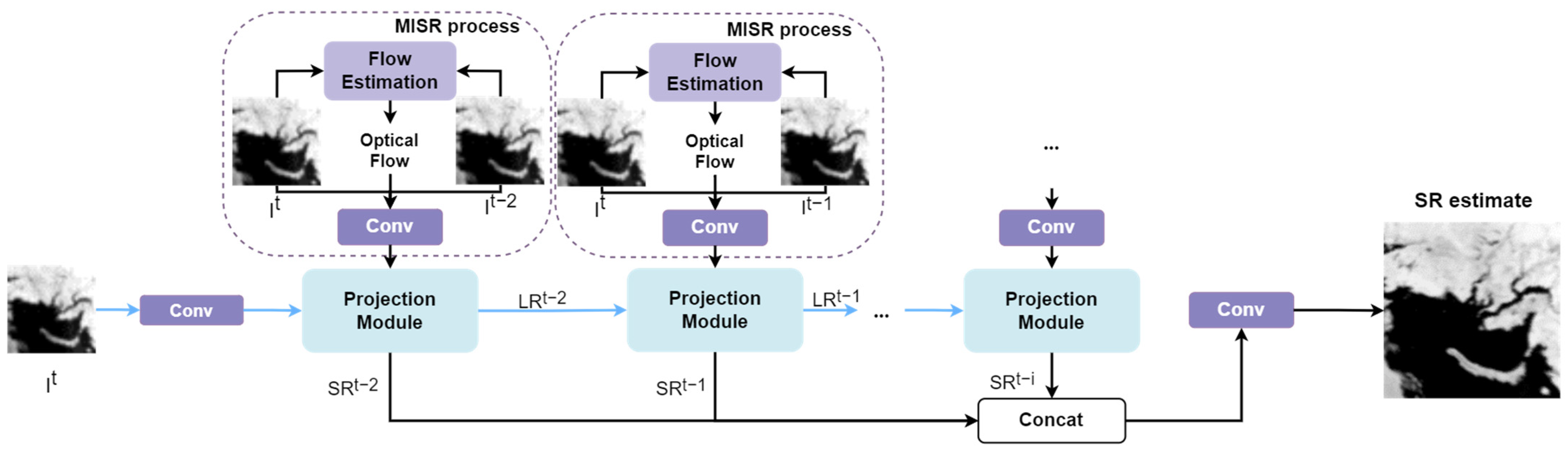
By analyzing the characteristics of passive microwave imagery and sea ice scenes, this study selects four state-of-the-art MISR networks, namely EDVR, PFNL, RBPN, and RRN. These networks are effectively applied to AMSR2 passive microwave imagery, resulting in a four-fold improvement in spatial resolution. It provides new ideas for improving the spatial resolution of passive microwave images, which enables a more accurate analysis of the Arctic sea ice.

(2)

The optimal length of the input image sequence of four MISR networks in different frequency bands is given. Additionally, the performances of each MISR network are evaluated at its respective optimal input sequence length for different frequency bands of passive microwave images. These findings offer valuable recommendations for selecting the appropriate MISR networks in different frequency bands of passive microwave imagery.

(3)

The quantification of the various impact factors on SR performance is also discussed in this paper. These impact factors include differences in sea ice concentration across different seasons, the influence of different magnitudes of sea ice motion, and the influence of different polarization modes of the images. By analyzing these factors, a deeper understanding of their effects on MISR performance is gained. This analysis provides insights into optimizing MISR algorithms for passive microwave sea ice imagery.

The remainder of this paper is organized as follows. Section 2 briefly introduces the image data used in this paper and the preparation of image datasets. Section 3 specifically describes the structures of the four SR networks used in this paper. Section 4 presents the experimental results and discussions. Conclusions are drawn in Section 5.

2. Materials

2.1. AMSR2 Images and Data Processing

AMSR2, an improved successor of the Advanced Microwave Scanning Radiometer–Earth Observing System (AMSR-E), is onboard the Global Change Observation Mission 1st-Water (GCOM-W1) satellite of the Japan Aerospace Exploration Agency (JAXA) as part of the global change observation mission [39,40,41]. The mission aims to observe the physical parameters connected with water and energy cycles on a global scale, with a particular focus on parameters such as SIC and total precipitation [39,42]. AMSR2 has seven frequencies, including 6.925 GHz, 7.3 GHz, 10.65 GHz, 18.7 GHz, 23.8 GHz, 36.5 GHz, and 89 GHz, each with two polarization modes, horizontal and vertical polarization [43,44,45]. The sampling interval and the size of the footprint at each frequency of AMSR2 are shown in

Table 1. Channel Specifications of AMSR2.

Frequency (GHz)	Sampling Interval (km)	Polarization	Footprint (Along-Scan × Along-Track) (km)
6.925/7.3	10	V/H	35 × 62
10.65	10	V/H	24 × 42
18.7	10	V/H	14 × 22
23.8	10	V/H	15 × 26
36.5	10	V/H	7 × 12
89	5	V/H	3 × 5

. At frequencies of 18.7 GHz, 36.5 GHz, and 89 GHz, they are the primary frequency bands for retrieving SIC due to their high sensitivity to the radiated signals of sea ice [46]. Therefore, only AMSR2 data at these three frequencies are involved in the following SR experiments.

In this paper, the L3 brightness temperature products from the AMSR2 sensor are used. The L3 product is a daily average version of the L1B brightness temperature product, which is gridded to the polar stereographic grids of the National Snow and Ice Data Center (NSIDC). The grid resolution of L3 brightness temperature products is 10 km.

The coverage of each image used in the paper is shown in Figure 1. The image size is 720 × 720 pixels, with a bit depth of 16-bit. The vertically polarized and horizontally polarized images are presented as separate images. We perform a cropping operation on the images, with each image cropped into patches of 180 × 180 pixels as the high-resolution (HR) images in the dataset. For the low-resolution (LR) images, we perform the bicubic downsampling operation with a scaling factor of 4 on the HR image dataset to obtain LR images of size 45 × 45 pixels. The training dataset covers the period from 2013 to 2016. Based on the length of the image input, we generate 23,324 LR image sequences and their corresponding HR images at each frequency with two polarization modes. The test dataset includes images in 2017 and 2022, which have 11,680 LR image sequences and their corresponding HR images at each frequency with two polarization modes.

In the training process, the LR image sequences are fed into the network as LR input with different input sequence lengths. The HR images corresponding to the center image of the LR image sequence (e.g., the third image when the image sequence length is 5) serve as the ground truth for training. As for the testing process, the LR image sequences in the test dataset are fed into the networks, which will output the SR image corresponding to the center image of the LR sequences. The performance of the network is then evaluated by comparing the evaluation criteria of SR and HR images.

2.2. Sea Ice Products

The SIC products [18] from the University of Bremen are used as the reference data for quantitatively comparing the proportion of sea ice at different seasons. The products have been continuously providing SIC data since 2002. The Arctic Radiation and Turbulence Interaction Study (ARTIST) Sea Ice (ASI) algorithm is utilized to retrieve the SIC data, calculated by the polarization difference of brightness temperature at 89 GHz, where the gradient ratios of channel pairs (e.g., 36.5 V and 18.7 V) are introduced for reducing the weather influences [18]. The spatial reference of the product is the polar stereographic projection of the NSIDC, with a spatial resolution of 6.25 km. The spatial coverage of the products used in this paper is consistent with Subregion 1 in the Kara Sea, as shown in Figure 1, and the dates are 25 February, 10 June, 3 July, and 19 November 2022.

The Polar Pathfinder Daily 25 km Equal-Area Scalable Earth (EASE)-Grid Sea Ice Motion Vector product [47] from NSIDC is used for quantitative comparison at different magnitudes of sea ice motion. This product contains weekly sea ice motion vectors. The input data which contain Advanced Very High-Resolution Radiometer (AVHRR), AMSR-E, SMMR, SSMI, and SSMI/S sensors images, International Arctic Buoy Programme (IABP) buoys’ data, and National Center for Environmental Prediction (NCEP)/National Center for Atmospheric Research (NCAR) reanalysis forecasts data, are used for retrieving the sea ice motion fields. The maximum cross-correlation (MCC) method [48] is used for retrieving sea ice vectors from remote sensing images, and the vectors from the reanalysis forecast data are calculated using the general rule proposed by Thorndike and Colony [49]. The vectors from the buoy data are calculated according to the distance at which the buoy’s position changes over 24 h. A cokriging estimation method [50] is employed for merging the vectors obtained above with minimal estimation error variance. The sea ice motion fields are then gridded to the EASE-Grid of the NSIDC at a gridding space of 25 km. In this paper, the product is reprojected to the Polar Stereographic grid of the NSIDC for consistent spatial reference. The spatial coverage of the sea ice motion vector product used in this paper is consistent with the Subregion in the Fram Strait, as shown in Figure 1, and the dates are 12–18 February and 19–25 March 2022.

3. SR Networks

In this paper, we compare the four selected MISR networks for SR performance on passive microwave imagery. First, the AMSR2 LR sequences and their corresponding HR images at each frequency band are fed into the network for training with different input lengths of image sequences. Then, the SR performances of the networks obtained with optimal input lengths are compared to obtain the best model for each MISR network. Next, the best models of the four MISR networks are further compared to find the best MISR method at each frequency band. Furthermore, the best models of the four networks are used to conduct experiments comparing the effects of various factors on SR performance.

The structures of the four networks used in this paper are shown in Figure 2, Figure 3, Figure 4 and Figure 5, and all the networks are illustrated using the input length of 5 as an example. As shown in Figure 2, the network of EDVR can be divided into three parts: Pyramid, Cascading, and Deformable convolutions (PCD) align module, Temporal and Spatial Attention (TSA) fusion module, and image reconstruction module. The PCD module utilizes deformable convolution to align the features. It makes the feature alignment more adaptable to the shape of the target in the image, which may tackle the complex deformations of sea ice. The module performs alignment between images in a coarse-to-fine manner by using the pyramid strategy to handle multi-scale motions, especially large motions. After the regular pyramid structure, the network also cascades an additional deformable alignment operation to refine the aligned features further, which improves the alignment accuracy. After being processed by the PCD module, the features on the neighboring images are aligned with the features on the reference image. The Spatiotemporal attention mechanism is adopted in the TSA fusion module when the aligned features are fused. The utilization of the spatiotemporal attention mechanism offers the benefit of making the network’s attention toward relevant feature information correlated with the reference image, including inter-frame temporal relation and intra-frame spatial relation. This mitigates the influence of erroneous information on the SR results. The fused features are used to reconstruct the residual SR image using a cascade of residual blocks in the reconstruction module. Finally, the residual SR image is added to the upsampled reference image to obtain the final SR image.

The structure of PNFL is shown in Figure 3a. The LR images are processed first by the Non-Local Residual Blocks (NLRBs) and convolution layer. The NLRBs exhibit an enhanced capability in capturing large-scale spatiotemporal correlations. This enhanced ability is achieved through computing correlations between features across every potential position and target feature. Additionally, it aligns images implicitly, which can be independent of the accuracy of motion estimation and compensation between sequential images, thereby further improving the SR results. The image features are then processed by a series of Progressive Fusion Residual Blocks (PFRBs). In each PFRB, illustrated in Figure 3b, the features of the LR images are progressively fused by multiple convolution and concatenation operations. In this progressive fusion process, in which the features of different images are fused twice in a PFRB, the spatial information within each image and the temporal information in the sequential images can be effectively used. Then, the network merges the information from the PFRBs and further generates a residual SR image. Finally, the SR image is generated by adding the residual SR image to the bicubically magnified image of the LR target image.

The workflow of the RBPN method is illustrated in Figure 4. In the SISR processes, which correspond to the blue arrows, the LR features are super-resolved to generate the SR features. For the MISR processes, the network generates the SR features of the reference image and each neighboring image ${\mathrm{I}}^{\mathrm{t}-\mathrm{i}}(\mathrm{i}=\pm 1, \pm 2)$ separately. The network uses the back-projection module to combine the SR features obtained from SISR and MISR processes for more complementary information in the image sequences. By iteratively back-projecting the features, the network generates the SR features ${\mathrm{S}\mathrm{R}}^{\mathrm{t}-\mathrm{i}}\left(\mathrm{i}=\pm 1,\pm 2\right)$ and the down-sampled SR features ${\mathrm{L}\mathrm{R}}^{\mathrm{t}-\mathrm{i}}\left(\mathrm{i}=\pm 1,\pm 2\right)$ in each step. The ${\mathrm{L}\mathrm{R}}^{\mathrm{i}}$ will be used as the SISR input in the next step. By fusing the reference image with each neighboring image separately, the time scale of the network can be expanded, enabling more effective utilization of neighboring image information even if the time span between the neighboring image and the reference image is large [37]. Moreover, it utilizes optical flow, which is concatenated with the image pairs, only as motion information in the image for implicit image alignment rather than for explicit motion compensation, which benefits the SR results. Finally, all generated SR features are concatenated and passed through convolutional layers to ultimately output the SR image.

The workflow of RRN is shown in Figure 5. The RRN belonging to the RNN-based method excels in handling long-term sequential image features, which can be beneficial for enriching the feature information. Typically, three parts are required as input at the time step t of the RRN: (1) the output ${\mathrm{O}}^{\mathrm{t}-1}$ of the previous step, (2) the hidden state feature ${\mathrm{h}}^{\mathrm{t}-1}$ of the previous step, and (3) the reference image and neighbor images [${\mathrm{I}}^{\mathrm{t}-1},{\mathrm{I}}^{\mathrm{t}}$]. When $\mathrm{t}=1$, the input just remains two parts: the initial hidden state of the network and the image pair of the reference image and the first neighbor image. The above inputs will go through multiple convolutional and ReLU layers to finally generate the output ${\mathrm{O}}_{\mathrm{t}}$ and hidden state ${\mathrm{h}}_{\mathrm{t}}$ for this step. The conv layers in light blue indicate that a ReLU layer is followed. It is worth mentioning that the RRN adopts residual mapping between convolutional layers with identity skip connections to address the issue of gradient vanishing and enhance the training stability. By incorporating residual learning in the network, the RRN can preserve more historical information over long periods and ensure a more information flow for easier handling of the longer image sequences [38]. This can overcome the problem of missing details in the image sequences by using previous information provided by the network. The final SR image is generated through the depth-to-space layer using the output of the final step and then added to the upsampled LR target image.

4. Results

4.1. Parameters Setting

All four SR networks used in this paper are finetuned using two NVIDIA GTX1080 GPUs. EDVR, RBPN, and RRN are implemented on the PyTorch framework, while PFNL is implemented on the TensorFlow framework. The networks super-resolve the image with an upscaling factor of 4 in the experiment. The parameters of four networks are optimized using the Adam optimizer with β1 = 0.9 and β2 = 0.999. The learning rate is set to ${10}^{-4}$ and the batch size is set to 8. All four networks employ the pixel-level loss function to measure the reconstruction errors between the predicted image and the truth. RBPN and RRN employ the L1 loss function, which calculates the absolute error between the truth and the predicted value. PFNL and EDVR use a variant of L1 loss known as Charbonnier loss [51], which is more robust by performing a square root calculation for the sum of squaring the error between the truth and the predicted value and a constant ${\mathsf{\epsilon }}^2$ [52,53]. The constant is introduced to avoid discontinuities in the loss function when the error is small. The ε is set to 0.001 in the experiment.

4.2. Evaluation Criterion

Two commonly used quantitative metrics, the Peak Signal Noise Ratio (PSNR) and the Structure Similarity Index Measure (SSIM), are utilized to evaluate the SR results of different SR networks. PSNR evaluates the errors between HR and SR images pixel by pixel. The higher the PSNR value, the smaller the differences in pixel level between the SR image and the reference HR image, and the higher the quality of the SR image. SSIM measures image structural similarity by calculating multiple factors such as brightness, contrast, and structure of the entire image, which can reflect the human perception of the image. The calculation methods of these two indicators are shown in Equations (1)–(3).

$$\mathrm{P}\mathrm{S}\mathrm{N}\mathrm{R}=10\times {\log }_{10}\left(\frac{2^n-1}{\mathrm{M}\mathrm{S}\mathrm{E}}\right)$$

(1)

$$\mathrm{S}\mathrm{S}\mathrm{I}\mathrm{M}=\frac{\left(2\times {\mathsf{\mu }}_{\mathrm{H}\mathrm{R}}\times {\mathsf{\mu }}_{\mathrm{S}\mathrm{R}}+{\mathrm{C}}_1\right)(2\times {\mathsf{\sigma }}_{\mathrm{H}\mathrm{R},\mathrm{S}\mathrm{R}}+{\mathrm{C}}_2)}{\left({{\mathsf{\mu }}_{\mathrm{H}\mathrm{R}}}^2+{{\mathsf{\mu }}_{\mathrm{S}\mathrm{R}}}^2+{\mathrm{C}}_1\right)\left({{\mathsf{\sigma }}_{\mathrm{H}\mathrm{R}}}^2+{{\mathsf{\sigma }}_{\mathrm{S}\mathrm{R}}}^2+{\mathrm{C}}_2\right)}$$

(2)

$${\mathrm{C}}_{\mathrm{i}}={\left({\mathrm{k}}_{\mathrm{i}}{\times (2}^{\mathrm{n}}-1\right))}^2\left(\mathrm{i}=1,2\right)$$

(3)

where MSE is the mean square error between the reconstructed SR image and the reference HR image, and n is the number of bits of the image. ${\mathsf{\mu }}_{\mathrm{S}\mathrm{R}}$, ${\mathsf{\mu }}_{\mathrm{H}\mathrm{R}}$, ${\mathsf{\sigma }}_{\mathrm{S}\mathrm{R}}$, and ${\mathsf{\sigma }}_{\mathrm{H}\mathrm{R}}$ represent the mean grayscale values and the variances of grayscale values of the reconstructed SR image and the reference HR images, respectively. ${\mathsf{\sigma }}_{\mathrm{H}\mathrm{R},\mathrm{S}\mathrm{R}}$ represents the covariance between the SR images and HR images. ${\mathrm{C}}_1$ and ${\mathrm{C}}_2$ are calculated by ${\mathrm{k}}_1$and ${\mathrm{k}}_2$. In this paper, ${\mathrm{k}}_1$and ${\mathrm{k}}_2$ are set to 0.01 and 0.03, respectively.

4.3. SR Results

4.3.1. Optimal Image Sequence Length and Best Network for Images at Different Frequencies

The number of images in a sequence input in MISR may influence the performance of the SR network. The optimum input image sequence length may vary when performing different MISR networks due to the differences in the ability to capture spatio-temporal features in image sequence for different SR networks. Therefore, the length of the input image sequence is used as a hyperparameter to discuss the optimal SR capability of each SR network. The length of the image sequence is set to 3, 5, 7, and 9, respectively, to train and test each MISR network. It is worth mentioning that the experiments with an input image sequence length of 9 for PFNL are not involved since the available maximum length of the input image sequence is 7.

Table 2. Results of PSNR/ SSIM on the test dataset for different lengths of the input image sequence in each frequency band for four MISR networks. The results in bold represent the results corresponding to the optimal length of input image sequence for each MISR network in each frequency band. The results underlined represent the best SR network results for each frequency band. The “-” indicates that there is no data.

Frequency (GHz)	Length of the Input Image Sequence	MISR Network
		EDVR	PFNL	RBPN	RRN
18.7	3	31.56/0.8779	39.58/0.9624	40.65/0.9491	41.53/0.9435
	5	36.09/0.9325	39.81/0.9639	40.82/0.9504	41.69/0.9745
	7	35.21/0.9305	40.44/0.9674	40.86/0.9522	41.78/0.9750
	9	35.64/0.9322	-	40.22/0.9492	41.74/0.9747
36.5	3	31.56/0.8297	37.10/0.9208	38.09/0.9254	38.73/0.9395
	5	35.27/0.8965	37.27/0.9232	38.51/0.9311	38.88/0.9411
	7	35.04/0.8948	36.63/0.9155	38.55/0.9312	39.06/0.9434
	9	35.24/0.8911	-	37.98/0.9249	38.91/0.9417
89	3	36.50/0.8879	36.54/0.8862	37.18/0.8935	37.73/0.9057
	5	39.64/0.9501	36.62/0.8879	37.26/0.8953	37.72/0.9057
	7	41.69/0.9505	36.57/0.8866	37.15/0.8931	38.00/0.9115
	9	41.56/0.9491	-	37.12/0.8924	37.99/0.9113

shows the quantitative evaluation results of the SR results of each network on the test dataset.

Firstly, the optimal length of the input image sequence for the four MISR networks can be found by comparing the SR results obtained with different input image sequence lengths in different frequency bands. As shown in Table 2, the best SR results for each MISR network in different frequency bands are represented in bold. It can be found that the SR performances do not improve as the length of the input increases. When the length of the image sequence is longer than the ability of the network to extract the spatiotemporal complementary information, the SR performance will instead decrease. Therefore, the best results will be obtained when the input length of the image sequence and the network’s ability to acquire spatiotemporal complementary information are matched.

According to Table 2, the optimal length of the input image sequence for the RRN network is 7 for all frequency bands, but the other three networks are 5 or 7, which confirms that RRN has the advantage of processing relatively long time series of images to improve SR results. It is able to combine the information in the time series and preserve the more effective information over long periods to obtain more valid spatiotemporal information. For EDVR, the optimal input length at 18.7 GHz is 5 and achieves performance improvements at 5.47 dB/0.0546 (PSNR/SSIM), 0.88 dB/0.0020, and 0.45 dB/0.0003, compared to the input length of 3, 7, and 9, respectively. At 36.5 GHz, the optimal input length is also 5, and the improvements are relatively modest than that at 18.7 GHz. However, at 89 GHz, the optimal input length is 7, and the SR results are comparable to when the input length is 9, and higher than both the lengths are 3 and 5. For PFNL, the optimal input lengths are 7, 5, and 5 at 18.7 GHz, 36.5 GHz, and 89 GHz, respectively. At 18.7 GHz, the PSNR/SSIM increases by up to 0.86 dB/0.0050 at the best input length compared to other input lengths. The worst SR result at 36.5 GHz is with an input length of 7, with a 0.64 dB/0.0077 performance degradation compared to the best result. At the 89 GHz frequency band, the differences in SR results are relatively small as the input length changes, with the maximum PSNR/SSIM difference not exceeding 0.08 dB/0.0017. For RBPN, the optimal input lengths at 18.7 GHz and 36.5 GHz are 7, and the performances are slightly higher than that at the input length of 5. In both bands, the worst result occurs at the input length of 9, with 0.64 dB/0.0030 and 0.57 dB/0.0063 degradation from the best result, respectively. The best result is obtained with an input length of 5 at 89 GHz, followed by the result at the length of 3, and the worst result is still obtained with an input length of 9, but overall, the differences in the result are marginal. For RRN, the optimal input lengths at all frequency bands are 7, and the results show an insignificance difference from the results for other input lengths. In addition, the results are almost the worst at the input length of 3, except at 89 GHz, where the PSNR at the input length of 3 is 0.01 higher than that at the input length of 5, but such a difference is ignorable.

It is worth mentioning that for the last three networks in Table 2, with the same image input length, the SR results achieve the best at 18.7 GHz while the worst at 89 GHz for each network. Here, we infer that this is because of the differences in the amount of information contained in the different frequencies of images. The footprint of the higher frequency image is smaller, which provides more and finer information in the image. The networks have similar capabilities in extracting image information for different frequencies, and high-frequency images contain more information, but they also include a higher amount of interference information, so the SR results are worse in high-frequency images. However, the EDVR performs best at 89 GHz. This may be because the network uses a spatiotemporal attention mechanism that allows filtering out more useless and distracting information, such as the water vapor interference in 89 GHz images, allowing the network to handle longer time series to extract effective information to achieve better SR results.

The SR results of four MISR networks in each frequency band by using the optimal length of the input image sequence are further compared. The best MISR network for each frequency band image is found (refer to the results marked with underline in Table 2). Among the four MISR methods, the RRN achieves the best SR result in both 18.7 GHz and 36.5 GHz frequency bands. In frequency 18.7 GHz, RRN achieves performance improvements of 5.69 dB/0.0425, 1.34 dB/0.0076, and 0.92 dB/0.0228 compared with EDVR, PFNL, and RBPN, respectively. In frequency 36.5 GHz, the improvements are 3.79 dB/0.0462, 1.79 dB/0.0202, and 0.51 dB/0.0124 compared with EDVR, PFNL, and RBPN, respectively. However, for the 89 GHz frequency band, the images are affected by water vapor and other atmospheric factors. The RRN network is unable to match neighboring images accurately and effectively due to water vapor occlusion during image reconstruction, which affects the image fusion and image reconstruction results. However, the results of the RRN are still better than those of RBPN and PFNL and just worse than those of EDVR. The EDVR network employs a spatiotemporal attention mechanism to counter the interference of water vapor. This may make the EDVR network superior to other MISR networks in SR results at 89 GHz. Liu [15] also compared the EDVR and RBPN networks for the 89 GHz images when setting the length of the input image sequence as 5, and the results were consistent with our results, where EDVR was better than RBPN.

4.3.2. Comparison of SR Results in Different Seasons

The spatial distribution of the Arctic sea ice exhibits significant variations across different seasons. Moreover, the extent of sea ice has considerably decreased in recent years due to global change, leading to further disparities in its spatial distribution. These distinct distribution patterns impact the feature alignment of image sequences, consequently influencing the performance of SR networks [54,55]. To quantitatively assess these effects, the disparities in SR results obtained from images acquired during different seasons are investigated. The seasons in the Arctic are usually divided into winter (January to March), spring (April to June), summer (July to September), and autumn (October to December) [20]. In each season, about 1440 LR test image sequences and corresponding HR images are contained for each frequency band, and the quantitative comparisons of SR results are shown in

Table 3. Quantitative comparison (PSNR/SSMI) of SR results of four MISR networks on the test dataset during different seasons of a year at each frequency. The best and worst results in different seasons are represented in red and blue, respectively.

Frequency (GHz)	Seasons	MISR Network
		EDVR	PFNL	RBPN	RRN
18.7	Winter	39.05/0.9540	40.28/0.9641	42.87/0.9741	42.97/0.9769
	Spring	36.84/0.9394	38.27/0.9515	40.97/0.9687	41.09/0.9759
	Summer	34.57/0.9237	36.16/0.9394	40.66/0.9715	41.00/0.9710
	Autumn	37.04/0.9435	38.34/0.9552	42.04/0.9738	42.05/0.9761
36.5	Winter	36.08/0.9085	37.32/0.9224	38.16/0.9219	39.05/0.9531
	Spring	34.79/0.8915	36.32/0.9123	37.30/0.9241	38.94/0.9373
	Summer	34.38/0.8928	35.77/0.9114	36.85/0.9196	38.38/0.9360
	Autumn	35.83/0.8932	37.12/0.9160	37.58/0.9223	39.19/0.9435
89	Winter	43.07/0.9628	37.95/0.9160	38.77/0.9230	39.52/0.9342
	Spring	41.12/0.9487	36.53/0.8905	37.04/0.8952	37.69/0.9092
	Summer	40.98/0.9424	35.96/0.8706	36.56/0.8811	37.34/0.8989
	Autumn	41.36/0.9481	36.06/0.8742	36.68/0.8821	37.45/0.9036

. The best and worst SR results for each MISR network in each frequency band are represented in red and blue, respectively. PSNR is primarily used for comparison and SSIM as a reference since PSNR is an index for comparing the similarity between HR and SR images pixel by pixel. According to Table 3, it can be found that for all frequency bands and all MISR networks, most of the best SR results are obtained in winter, while the worst are in summer. At the frequency of 18.7 GHz, the EDVR, RBPN, PFNL, and RNN exhibit superior SR results in winter compared to summer by 4.48 dB (PSNR), 4.12 dB, 2.21 dB, and 1.97 dB, respectively. At the frequency of 36.5 GHz, the result differences are relatively small, with the largest difference being 1.70 dB for EDVR and the smallest being 0.67 dB for RNN. At the frequency of 89 GHz, the performance gaps of different seasons for all four networks are relatively close, which are around 2.00 dB. The possible reason is that the Arctic sea ice region scene becomes more complex during summer [56,57], as large areas of Arctic sea ice melt into open water. Consequently, environmental factors, such as surface wind, may introduce disruptive features, such as ripples on the water surface in sequential images. These disturbances may adversely affect the quality of SR results. In addition, the sea ice scene changes rapidly in summer, such as the generation of melt ponds, rapid changes in sea ice morphology, etc., as well as the seriousness of water vapor in summer. These factors may also affect the SR results in summer. It is worth noting that when applying the RRN model to images at 36.5 GHz, although our main evaluation metric, PSNR, is slightly higher in the autumn than in the winter, the trend for the whole year still shows that the SR results are better in winter than in summer.

An area in the Kara Sea (Subregion 1 in Figure 1) is selected to show the differences in SR results in different seasons. It is mostly covered by sea ice in winter in this area, and a large part of the ice-covered area will melt to form open water in summer. The SIC products, provided by the University of Bremen (downloaded at https://seaice.uni-bremen.de, accessed on 13 November 2023), are used for quantitative comparison of the proportion of sea ice in this area at different seasons. Four images at different seasons, obtained on 25 February, 10 June, 3 July, and 19 November 2022, with average SIC of 81.79%, 56.18%, 17.36%, and 57.80%, respectively, are used to compare the SR results.

Table 4. Quantitative results of the four networks in the Kara Sea region (Subregion 1 in Figure 1) on different dates at all frequencies. Results in bold represent the best PSNR and SSIM.

Frequency (GHz)	Date	MISR Framework
		EDVR	PFNL	RBPN	RRN
18.7	25 February	43.47/0.9716	44.64/0.9769	44.77/0.9794	46.85/0.9842
	10 June	36.97/0.9044	37.81/0.9494	38.96/0.9326	39.12/0.9474
	3 July	36.33/0.9016	37.57/0.9308	38.66/0.9323	38.76/0.9400
	19 November	42.21/0.9527	43.13/0.9735	43.84/0.9752	45.24/0.9795
36.5	25 February	42.45/0.9734	43.02/0.9649	43.19/0.9660	43.37/0.9678
	10 June	37.75/0.9071	38.75/0.9279	38.87/0.9540	39.09/0.9513
	3 July	35.96/0.8849	37.81/0.9254	38.17/0.9251	38.28/0.9255
	19 November	40.74/0.9530	42.29/0.9617	42.07/0.9555	42.34/0.9573
89	25 February	45.32/0.9731	43.43/0.9655	44.21/0.9703	45.17/0.9728
	10 June	44.88/0.9691	43.28/0.9655	43.78/0.9510	43.97/0.9603
	3 July	43.91/0.9658	41.61/0.9387	41.89/0.9483	42.06/0.9400
	19 November	44.03/0.9649	41.67/0.9445	42.00/0.9503	42.45/0.9588

shows the quantitative comparison of the SR results in each frequency band by using four MISR networks. As marked in bold in Table 4, the results show that all four MISR networks achieved better SR results for the image from 25 February (in winter). Take the images at 18.7 GHz in vertical polarization as an example; the visual comparisons of SR results in this area are given in Figure 6. The extent of Subregion 1 is marked with a solid red box, and the quantitative metrics (PSNR/SSMI) are displayed above the box. It is shown that all four networks improve the detail of the image compared with the LR images. Especially in the regions of water-land boundaries and ice floes, the edge details within these areas become more pronounced. According to the results, the images from 25 February and 19 November achieved better results than the images from 10 June and 3 July. In the images on 10 June and 3 July, there is more crushed ice, which is more susceptible to movement under the influence of environmental factors, e.g., wind, resulting in poor SR results to some extent. Compared to the other three methods, the SR results of EDVR are noisier (bright spots in the image) and blurred, with less high-frequency detail, and show the worst SR results in four seasons at 18.7 GHz. Although there is a minimal disparity in visual comparison between RRN, RBPN, and PFNL, RRN demonstrated a smaller variance from the ground truth imagery, containing fewer instances of erroneous information, and achieved the best quantitative results.

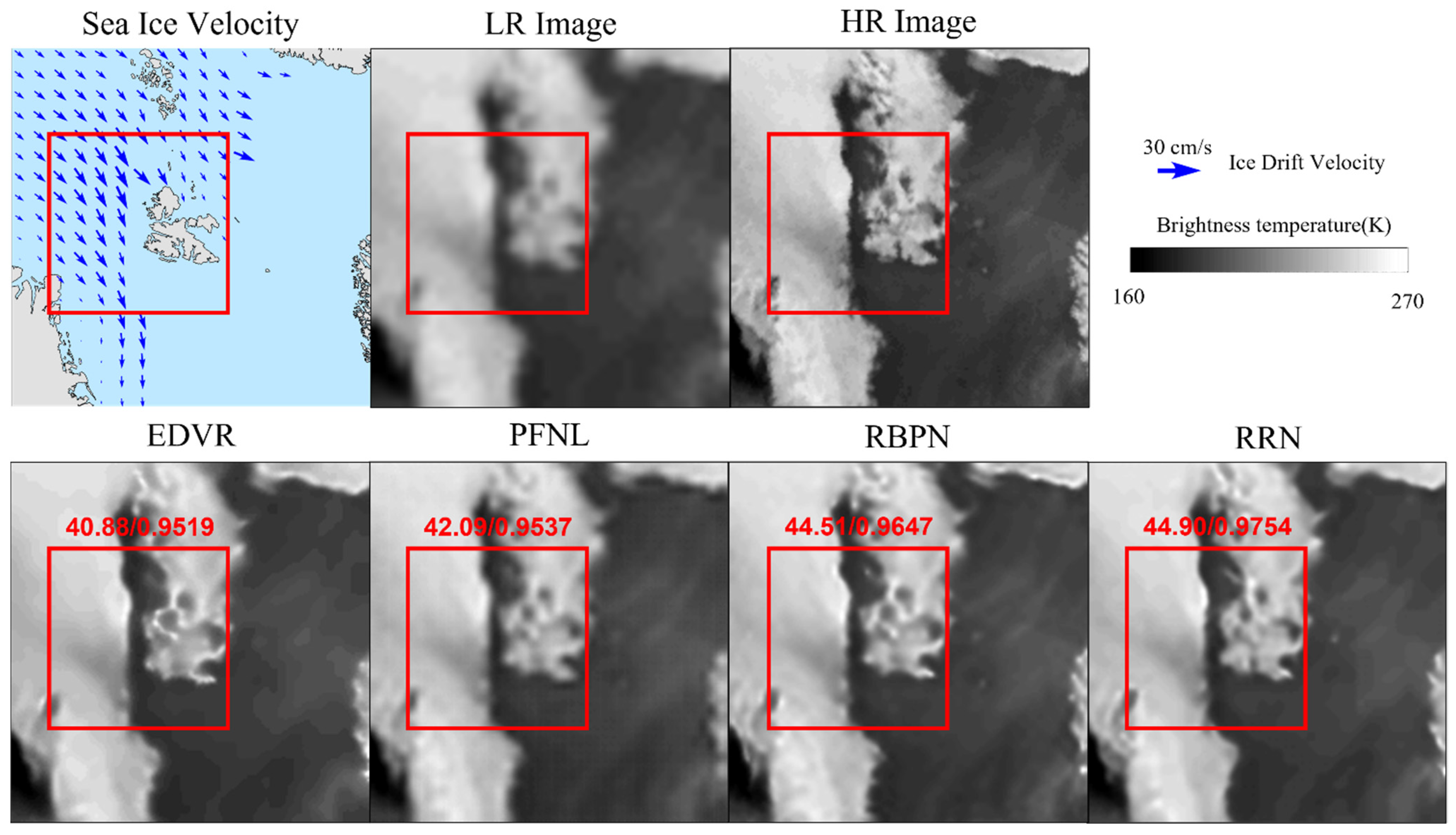
4.3.3. Comparison of SR Results with Different Ice Motion Velocity

The spatial variation in features in sequential images caused by the motion of sea ice is a crucial factor influencing the results of image SR. Furthermore, global climate change has resulted in a decrease in sea ice thickness, potentially leading to accelerated sea ice movement. These rapid and extensive motions pose challenges for motion estimation and compensation. Additionally, the inaccurate feature alignment can further result in unsatisfactory SR performance [58,59]. Considering the transpolar drift phenomenon in the Arctic, sea ice movement in Fram Strait is particularly active, and Arctic sea ice often flows from Fram Strait into the Atlantic Ocean [60]. Therefore, this region (as shown in Subregion 2 in Figure 1) is selected to investigate the influence of the difference in sea ice motion in sequence images on the SR results. The images from 12–18 February and from 19–25 March 2022 are used for the comparison of SR results. The weekly Arctic sea ice motion product, downloaded from NSIDC (https://nsidc.org/data/nsidc-0748, accessed on 13 November 2023), is used to quantify the differences between average sea ice motion, which was 4.72 cm/s (4.08 km/d) and 11.31 cm/s (9.77 km/d) for 12–18 February and 19–25 March.

Table 5. Quantitative results of the four networks on the test set in Subregion 2 of the Fram Strait during periods of slow (15 February 2022) and fast (22 March 2022) sea ice motion at all frequencies. Bold results indicate the best PSNR and SSIM.

Frequency	Date	MISR Network
		EDVR	PFNL	RBPN	RRN
18	15 February	39.36/0.9404	40.49/0.9494	42.33/0.9665	43.20/0.9720
	22 March	38.41/0.9311	39.96/0.9494	40.89/0.9597	41.16/0.9605
36	15 February	41.49/0.9504	41.65/0.9527	42.24/0.9542	42.45/0.9577
	22 March	40.41/0.9430	41.48/0.9496	42.11/0.9497	42.44/0.9511
89	15 February	43.71/0.9662	43.21/0.9597	42.61/0.9499	43.21/0.9596
	22 March	43.11/0.9637	42.17/0.9482	41.60/0.9378	42.72/0.9549

shows the SR results of the four networks in different frequency bands in this Subregion. It can be found that the SR results of images with small sea ice motion (12–18 February) are better than those with large sea ice motion (19–25 March). Overall, the relatively fast sea ice motion may make the tracking of sea ice in image sequence more difficult and worsen the SR performance of the networks. Taking 18.7 GHz in the vertical polarization as an example, the visual comparison of SR results in this area on 15 February and 22 March are given in Figure 7 and Figure 8. For better visualization, we dilute the sea ice motion vectors by a factor of 4. The extent of Subregion 2 is marked with a solid red box, and the quantitative metrics (PSNR/SSIM) are displayed above the box. Comparing the SR effects of each network in different periods, the quantitative results of image SR during the slow sea ice motion period (12–18 February) are better than those during the fast sea ice motion period (19–25 March). Among the four networks, RRN performed the best. This might be due to the fact that during periods of sea ice motion, tracking sea ice features in the image sequences could become challenging, while the structure of RRN can retain more historical feature information when processing the image sequence to provide more information for the SR process. Although there are some numerical differences in the SR effects of the other three networks, there is not much difference in visual comparison.

4.3.4. Comparison of Different Polarization Modes

We conducted statistical analysis on the SR results of images with different polarization modes in the whole test set, as shown in

Table 6. Four networks are compared for their PSNR and SSIM results on images with different polarization modes in the test set. Results in bold represent the best PSNR and SSIM.

Polarization	MISR Network
	EDVR	PFNL	RBPN	RRN
H	37.54/0.9697	41.92/0.9846	42.70/0.9757	43.38/0.9878
V	41.97/0.9812	45.96/0.9896	46.38/0.9798	47.30/0.9915

. The quantitative indicators of SR results in all frequency bands are averaged to concisely compare the effect of SR results in the images of different polarization modes. Based on the results in Table 6, all methods demonstrated significantly better SR performance on vertically polarized images than on horizontally polarized images with quantitative differences of 4.43 dB/0.0115 (PSNR/SSIM), 4.04 dB/0.0050, 3.68 dB/0.0041, and 3.92 dB/0.0037, respectively. This may be related to the fact that the features of vertically polarized images are more distinct and easier for the network to extract, resulting in better SR performance compared to horizontally polarized images.

5. Conclusions

In order to overcome the spatial resolution limitation in passive microwave images and investigate appropriate MISR networks for passive microwave sea ice images at different frequencies, the applicability of the four competitive MISR networks, i.e., EDVR [35], PFNL [36], RBPN [37], and RRN [38], in multi-frequency AMSR2 passive microwave images for Arctic sea ice scenes are explored in this paper. The optimal input image sequence lengths for each MISR network in different frequency bands are given to find the best network model that can promote the development of MISR networks for passive microwave images. Moreover, the impacts of some influencing factors on the SR results are also discussed, and conclusions are drawn about the sea ice scenarios for which the SR networks are better suited. According to the results of extensive SR experiments, we can draw the following conclusions: (1) At frequencies of 18.7 GHz and 36.5 GHz, RRN is the best SR network with the optimal length of the input image sequence at 7, which produces fewer artifacts and more accurate boundaries in the images. For the images at frequency 89 GHz, which are often affected by water vapor, EDVR outperforms the other three networks by a minimum of 2.69 dB/0.039 in PSNR/SSIM, with the optimal number of input images of 7. (2) Seasonal variations in sea ice cover and sea ice morphology can affect SR performance of the networks. In general, SR results are better in winter, when sea ice is more stable than in summer, with the maximum PSNR difference of 2.04 dB. (3) The magnitude of the sea ice motion also has an impact on the accuracy of the image alignment during SR. For all four networks, the SR results under small sea ice motion are better than those under large sea ice motion. (4) The vertically polarized images have an advantage over horizontally polarized images in SR results, with an average improvement of 4.02 dB in PSNR and 0.0061 in SSIM. Overall, the results of this paper can provide new ideas and a reference for the selection of MISR networks to improve the spatial resolution of Arctic sea ice passive microwave images at different frequencies and demonstrate the quantification of the impact of images from different scenes and different polarization modes on SR results. However, there are differences between the natural images and passive microwave images, which limit the performance of the network used in this paper. In future research, it is necessary to develop an MISR network for passive microwave sea ice images at different frequency bands for further improvement of the SR performance in Arctic sea ice scenarios.

References

1. Comiso, J.C.; Parkinson, C.L.; Gersten, R.; Stock, L. Accelerated Decline in the Arctic Sea Ice Cover. Geophys. Res. Lett. 2008, 35, L01703. [Google Scholar] [CrossRef]
2. Huntemann, M.; Heygster, G.; Kaleschke, L.; Krumpen, T.; Mäkynen, M.; Drusch, M. Empirical Sea Ice Thickness Retrieval during the Freeze-up Period from SMOS High Incident Angle Observations. Cryosphere 2014, 8, 439–451. [Google Scholar] [CrossRef]
3. Haarpaintner, J.ö.; Spreen, G. Use of Enhanced-Resolution QuikSCAT/SeaWinds Data for Operational Ice Services and Climate Research: Sea Ice Edge, Type, Concentration, and Drift. IEEE Trans. Geosci. Remote Sens. 2007, 45, 3131–3137. [Google Scholar] [CrossRef]
4. Sommerkorn, M.; Hassol, S.J. Arctic Climate Feedbacks: Global Implications. In Arctic Climate Feedbacks: Global Implications; WWF International Arctic Programme: Washington, DC, USA, 2009. [Google Scholar]
5. Bintanja, R.; van Oldenborgh, G.J.; Drijfhout, S.S.; Wouters, B.; Katsman, C.A. Important Role for Ocean Warming and Increased Ice-Shelf Melt in Antarctic Sea-Ice Expansion. Nat. Geosci. 2013, 6, 376–379. [Google Scholar] [CrossRef]
6. Aagaard, K.; Carmack, E.C. The Role of Sea Ice and Other Fresh Water in the Arctic Circulation. J. Geophys. Res. Ocean. 1989, 94, 14485–14498. [Google Scholar] [CrossRef]
7. Cavalieri, D.J.; Parkinson, C.L. Arctic Sea Ice Variability and Trends, 1979–2010. Cryosphere 2012, 6, 881–889. [Google Scholar] [CrossRef]
8. Turner, J.; Bracegirdle, T.J.; Phillips, T.; Marshall, G.J.; Hosking, J.S. An Initial Assessment of Antarctic Sea Ice Extent in the CMIP5 Models. J. Clim. 2013, 26, 1473–1484. [Google Scholar] [CrossRef]
9. Boé, J.; Hall, A.; Qu, X. September Sea-Ice Cover in the Arctic Ocean Projected to Vanish by 2100. Nat. Geosci. 2009, 2, 341–343. [Google Scholar] [CrossRef]
10. Burek, K.A.; Gulland, F.M.; O’Hara, T.M. Effects of Climate Change on Arctic Marine Mammal Health. Ecol. Appl. 2008, 18, S126–S134. [Google Scholar] [CrossRef]
11. Laidre, K.L.; Stirling, I.; Lowry, L.F.; Wiig, Ø.; Heide-Jørgensen, M.P.; Ferguson, S.H. Quantifying the Sensitivity of Arctic Marine Mammals to Climate-Induced Habitat Change. Ecol. Appl. 2008, 18, S97–S125. [Google Scholar] [CrossRef]
12. Lee, S.-W.; Song, J.-M. Economic Possibilities of Shipping Though Northern Sea Route1. Asian J. Shipp. Logist. 2014, 30, 415–430. [Google Scholar] [CrossRef]
13. Peeken, I.; Primpke, S.; Beyer, B.; Gütermann, J.; Katlein, C.; Krumpen, T.; Bergmann, M.; Hehemann, L.; Gerdts, G. Arctic Sea Ice Is an Important Temporal Sink and Means of Transport for Microplastic. Nat. Commun. 2018, 9, 1505. [Google Scholar] [CrossRef] [PubMed]
14. Xian, Y.; Petrou, Z.I.; Tian, Y.; Meier, W.N. Super-Resolved Fine-Scale Sea Ice Motion Tracking. IEEE Trans. Geosci. Remote Sens. 2017, 55, 5427–5439. [Google Scholar] [CrossRef]
15. Liu, X.; Feng, T.; Shen, X.; Li, R. PMDRnet: A Progressive Multiscale Deformable Residual Network for Multi-Image Super-Resolution of AMSR2 Arctic Sea Ice Images. IEEE Trans. Geosci. Remote Sens. 2022, 60, 4304118. [Google Scholar] [CrossRef]
16. Duan, S.-B.; Han, X.-J.; Huang, C.; Li, Z.-L.; Wu, H.; Qian, Y.; Gao, M.; Leng, P. Land Surface Temperature Retrieval from Passive Microwave Satellite Observations: State-of-the-Art and Future Directions. Remote Sens. 2020, 12, 2573. [Google Scholar] [CrossRef]
17. Lindsay, R.W.; Rothrock, D.A. Arctic Sea Ice Leads from Advanced Very High Resolution Radiometer Images. J. Geophys. Res. 1995, 100, 4533. [Google Scholar] [CrossRef]
18. Spreen, G.; Kaleschke, L.; Heygster, G. Sea Ice Remote Sensing Using AMSR-E 89-GHz Channels. J. Geophys. Res. Ocean. 2008, 113, C02S03. [Google Scholar] [CrossRef]
19. Wernecke, A.; Kaleschke, L. Lead Detection in Arctic Sea Ice from CryoSat-2: Quality Assessment, Lead Area Fraction and Width Distribution. Cryosphere 2015, 9, 1955–1968. [Google Scholar] [CrossRef]
20. Zhang, F.; Pang, X.; Lei, R.; Zhai, M.; Zhao, X.; Cai, Q. Arctic Sea Ice Motion Change and Response to Atmospheric Forcing between 1979 and 2019. Int. J. Climatol. 2022, 42, 1854–1876. [Google Scholar] [CrossRef]
21. Meier, W.N.; Markus, T.; Comiso, J.C. AMSR-E/AMSR2 Unified L3 Daily 12.5 Km Brightness Temperatures, Sea Ice Concentration, Motion & Snow Depth Polar Grids, Version 1 2018. Available online: http://nsidc.org/data/AU_SI12/versions/1 (accessed on 13 November 2023).
22. Backus, G.E.; Gilbert, J.F. Numerical Applications of a Formalism for Geophysical Inverse Problems. Geophys. J. Int. 1967, 13, 247–276. [Google Scholar] [CrossRef]
23. Backus, G.; Gilbert, F. The Resolving Power of Gross Earth Data. Geophys. J. Int. 1968, 16, 169–205. [Google Scholar] [CrossRef]
24. Wang, P.; Bayram, B.; Sertel, E. A Comprehensive Review on Deep Learning Based Remote Sensing Image Super-Resolution Methods. Earth-Sci. Rev. 2022, 232, 104110. [Google Scholar] [CrossRef]
25. Wang, Z.; Chen, J.; Hoi, S.C.H. Deep Learning for Image Super-Resolution: A Survey. IEEE Trans. Pattern Anal. Mach. Intell. 2021, 43, 3365–3387. [Google Scholar] [CrossRef]
26. Yang, W.; Zhang, X.; Tian, Y.; Wang, W.; Xue, J.-H.; Liao, Q. Deep Learning for Single Image Super-Resolution: A Brief Review. IEEE Trans. Multimed. 2019, 21, 3106–3121. [Google Scholar] [CrossRef]
27. Petrou, Z.I.; Xian, Y.; Tian, Y. Towards Breaking the Spatial Resolution Barriers: An Optical Flow and Super-Resolution Approach for Sea Ice Motion Estimation. ISPRS J. Photogramm. Remote Sens. 2018, 138, 164–175. [Google Scholar] [CrossRef]
28. Hu, W.; Zhang, W.; Chen, S.; Lv, X.; An, D.; Ligthart, L. A Deconvolution Technology of Microwave Radiometer Data Using Convolutional Neural Networks. Remote Sens. 2018, 10, 275. [Google Scholar] [CrossRef]
29. Hu, W.; Li, Y.; Zhang, W.; Chen, S.; Lv, X.; Ligthart, L. Spatial Resolution Enhancement of Satellite Microwave Radiometer Data with Deep Residual Convolutional Neural Network. Remote Sens. 2019, 11, 771. [Google Scholar] [CrossRef]
30. Hu, T.; Zhang, F.; Li, W.; Hu, W.; Tao, R. Microwave Radiometer Data Superresolution Using Image Degradation and Residual Network. IEEE Trans. Geosci. Remote Sens. 2019, 57, 8954–8967. [Google Scholar] [CrossRef]
31. Li, Y.; Hu, W.; Chen, S.; Zhang, W.; Guo, R.; He, J.; Ligthart, L. Spatial Resolution Matching of Microwave Radiometer Data with Convolutional Neural Network. Remote Sens. 2019, 11, 2432. [Google Scholar] [CrossRef]
32. Liu, H.; Ruan, Z.; Zhao, P.; Dong, C.; Shang, F.; Liu, Y.; Yang, L.; Timofte, R. Video Super-Resolution Based on Deep Learning: A Comprehensive Survey. Artif. Intell. Rev. 2022, 55, 5981–6035. [Google Scholar] [CrossRef]
33. Salvetti, F.; Mazzia, V.; Khaliq, A.; Chiaberge, M. Multi-Image Super Resolution of Remotely Sensed Images Using Residual Attention Deep Neural Networks. Remote Sens. 2020, 12, 2207. [Google Scholar] [CrossRef]
34. Arefin, M.R.; Michalski, V.; St-Charles, P.-L.; Kalaitzis, A.; Kim, S.; Kahou, S.E.; Bengio, Y. Multi-Image Super-Resolution for Remote Sensing Using Deep Recurrent Networks. In Proceedings of the IEEE/CVF Conference on Computer Vision and Pattern Recognition Workshops 2020, Seattle, WA, USA, 14–19 June 2020; pp. 206–207. [Google Scholar]
35. Wang, X.; Chan, K.C.K.; Yu, K.; Dong, C.; Change Loy, C. EDVR: Video Restoration With Enhanced Deformable Convolutional Networks. In Proceedings of the Proceedings of the IEEE/CVF Conference on Computer Vision and Pattern Recognition (CVPR) Workshops, Long Beach, CA, USA, 14–20 June 2019. [Google Scholar]
36. Yi, P.; Wang, Z.; Jiang, K.; Jiang, J.; Ma, J. Progressive Fusion Video Super-Resolution Network via Exploiting Non-Local Spatio-Temporal Correlations. In Proceedings of the 2019 IEEE/CVF International Conference on Computer Vision (ICCV), Seoul, Republic of Korea, 27 October–2 November 2019; IEEE: Seoul, Republic of Korea, 2019; pp. 3106–3115. [Google Scholar]
37. Haris, M.; Shakhnarovich, G.; Ukita, N. Recurrent Back-Projection Network for Video Super-Resolution. In Proceedings of the 2019 IEEE/CVF Conference on Computer Vision and Pattern Recognition (CVPR), Long Beach, CA, USA, 14–20 June 2019; pp. 3892–3901. [Google Scholar]
38. Isobe, T.; Zhu, F.; Jia, X.; Wang, S. Revisiting Temporal Modeling for Video Super-Resolution. arXiv 2020, arXiv:2008.05765. [Google Scholar]
39. Imaoka, K.; Maeda, T.; Kachi, M.; Kasahara, M.; Ito, N.; Nakagawa, K. Status of AMSR2 Instrument on GCOM-W1. In Earth Observing Missions and Sensors: Development, Implementation, and Characterization II; SPIE: St Bellingham, WA, USA, 2012; Volume 8528, pp. 201–206. [Google Scholar]
40. Du, J.; Kimball, J.S.; Jones, L.A.; Kim, Y.; Glassy, J.; Watts, J.D. A Global Satellite Environmental Data Record Derived from AMSR-E and AMSR2 Microwave Earth Observations. Earth Syst. Sci. Data 2017, 9, 791–808. [Google Scholar] [CrossRef]
41. Ma, H.; Zeng, J.; Chen, N.; Zhang, X.; Cosh, M.H.; Wang, W. Satellite Surface Soil Moisture from SMAP, SMOS, AMSR2 and ESA CCI: A Comprehensive Assessment Using Global Ground-Based Observations. Remote Sens. Environ. 2019, 231, 111215. [Google Scholar] [CrossRef]
42. Oki, T.; Imaoka, K.; Kachi, M. AMSR Instruments on GCOM-W1/2: Concepts and Applications. In Proceedings of the 2010 IEEE International Geoscience and Remote Sensing Symposium, Honolulu, HI, USA, 25–30 July 2010; pp. 1363–1366. [Google Scholar]
43. Cui, H.; Jiang, L.; Du, J.; Zhao, S.; Wang, G.; Lu, Z.; Wang, J. Evaluation and Analysis of AMSR-2, SMOS, and SMAP Soil Moisture Products in the Genhe Area of China. J. Geophys. Res. Atmos. 2017, 122, 8650–8666. [Google Scholar] [CrossRef]
44. Kachi, M.; Hori, M.; Maeda, T.; Imaoka, K. Status of Validation of AMSR2 on Board the GCOM-W1 Satellite. In Proceedings of the 2014 IEEE Geoscience and Remote Sensing Symposium, Quebec City, QC, Canada, 13–18 July 2014; pp. 110–113. [Google Scholar]
45. Maeda, T.; Imaoka, K.; Kachi, M.; Fujii, H.; Shibata, A.; Naoki, K.; Kasahara, M.; Ito, N.; Nakagawa, K.; Oki, T. Status of GCOM-W1/AMSR2 Development, Algorithms, and Products. In Proceedings of the Sensors, Systems, and Next-Generation Satellites XV, Prague, Czech Republic, 19–22 September 2011; SPIE: St Bellingham, WA, USA, 2011; Volume 8176, pp. 183–189. [Google Scholar]
46. Imaoka, K.; Kachi, M.; Fujii, H.; Murakami, H.; Hori, M.; Ono, A.; Igarashi, T.; Nakagawa, K.; Oki, T.; Honda, Y.; et al. Global Change Observation Mission (GCOM) for Monitoring Carbon, Water Cycles, and Climate Change. Proc. IEEE 2010, 98, 717–734. [Google Scholar] [CrossRef]
47. Tschudi, M.W.N.; Meier, J.S.; Stewart, C.F.; Maslanik, J. Polar Pathfinder Daily 25 Km EASE-Grid Sea Ice Motion Vectors, 4th ed.; National Snow and Ice Data Center Address: Boulder, CO, USA, 2019. [Google Scholar]
48. Emery, W.J.; Fowler, C.W.; Maslanik, J. Satellite Remote Sensing. Oceanogr. Appl. Remote Sens. 1995, 23, 367–379. [Google Scholar]
49. Thorndike, A.S.; Colony, R. Sea Ice Motion in Response to Geostrophic Winds. J. Geophys. Res. Ocean. 1982, 87, 5845–5852. [Google Scholar] [CrossRef]
50. Isaaks, E.H.; Srivastava, R.M. Applied Geostatistics; Oxford University Press: Oxford, UK, 1989. [Google Scholar]
51. Charbonnier, P.; Blanc-Feraud, L.; Aubert, G.; Barlaud, M. Deterministic Edge-Preserving Regularization in Computed Imaging. IEEE Trans. Image Process. 1997, 6, 298–311. [Google Scholar] [CrossRef]
52. Lai, W.-S.; Huang, J.-B.; Ahuja, N.; Yang, M.-H. Fast and Accurate Image Super-Resolution with Deep Laplacian Pyramid Networks. IEEE Trans. Pattern Anal. Mach. Intell. 2019, 41, 2599–2613. [Google Scholar] [CrossRef]
53. Lai, W.-S.; Huang, J.-B.; Ahuja, N.; Yang, M.-H. Deep Laplacian Pyramid Networks for Fast and Accurate Super-Resolution. In Proceedings of the 2017 IEEE Conference on Computer Vision and Pattern Recognition (CVPR), Honolulu, HI, USA, 21–26 July 2017; IEEE: Piscataway, NJ, USA; pp. 5835–5843. [Google Scholar]
54. Chan, K.C.K.; Zhou, S.; Xu, X.; Loy, C.C. BasicVSR++: Improving Video Super-Resolution With Enhanced Propagation and Alignment. In Proceedings of the IEEE/CVF Conference on Computer Vision and Pattern Recognition (CVPR), New Orleans, LA, USA, 18–24 June 2022; pp. 5972–5981. [Google Scholar]
55. Tian, Y.; Zhang, Y.; Fu, Y.; Xu, C. TDAN: Temporally-Deformable Alignment Network for Video Super-Resolution. In Proceedings of the IEEE/CVF Conference on Computer Vision and Pattern Recognition (CVPR), Seattle, WA, USA, 13–19 June 2020; pp. 3360–3369. [Google Scholar]
56. Tang, C.C.L.; Ross, C.K.; Yao, T.; Petrie, B.; DeTracey, B.M.; Dunlap, E. The Circulation, Water Masses and Sea-Ice of Baffin Bay. Prog. Oceanogr. 2004, 63, 183–228. [Google Scholar] [CrossRef]
57. Stroeve, J.; Notz, D. Changing State of Arctic Sea Ice across All Seasons. Environ. Res. Lett. 2018, 13, 103001. [Google Scholar] [CrossRef]
58. Takeda, H.; Milanfar, P.; Protter, M.; Elad, M. Super-Resolution Without Explicit Subpixel Motion Estimation. IEEE Trans. Image Process. 2009, 18, 1958–1975. [Google Scholar] [CrossRef]
59. Brox, T.; Malik, J. Large Displacement Optical Flow: Descriptor Matching in Variational Motion Estimation. IEEE Trans. Pattern Anal. Mach. Intell. 2011, 33, 500–513. [Google Scholar] [CrossRef]
60. Kwok, R.; Rothrock, D.A. Variability of Fram Strait Ice Flux and North Atlantic Oscillation. J. Geophys. Res. Ocean. 1999, 104, 5177–5189. [Google Scholar] [CrossRef]
Figure 1. The coverage of each AMSR2 L3 gridded image was used to prepare the datasets in this paper. The gray area represents the land mask, the blue area represents oceans, and both the maximum sea ice extent (white area) and the boundary of minimum sea ice extent (light grey lines) in 2022, based on the sea ice extent products provided by NSIDC (https://nsidc.org/data/g02186/versions/1, accessed on 13 November 2023), are shown.
Remotesensing 15 05401 g001
Figure 2. The architecture of the EDVR network. Different shades of purple represent different features in the network. The arrows are the directions of operation in the network.
Remotesensing 15 05401 g002
Figure 3. (a) The architecture of the PFNL network; (b) The detailed structure of progressive fusion resblock. Different shades of purple represent different features in the network. The arrows are the directions of operation in the network.
Remotesensing 15 05401 g003
Figure 4. The architecture of the RBPN network. Different shades of purple represent different features in the network. The arrows are the directions of operation in the network.
Remotesensing 15 05401 g004
Figure 5. The architecture of the RRN network. Different shades of purple represent different features in the network. The arrows are the directions of operation in the network.
Remotesensing 15 05401 g005
Figure 6. Visual and quantitative comparison during four seasons in Subregion 1 near the Kara Sea (red box), with a scaling factor of 4. The SIC product, HR image, and LR image to be resolved were obtained on 25 February, 10 June, 3 July, and 19 November 2022. The quantitative results of each method are displayed at the top of the red box.
Remotesensing 15 05401 g006
Figure 7. Visual and quantitative comparisons are made in Subregion 2 (red box) near Fram Strait during a period of slow sea ice motion, with a scaling factor of 4. Sea ice velocity product was obtained on 12–18 February 2022, and HR images and the LR images to be resolved were obtained on 15 February 2022. The quantitative results for each method are displayed at the top of the red box.
Remotesensing 15 05401 g007
Figure 8. Visual and quantitative comparisons are made in Region 2 (red box) near Fram Strait during a period of fast sea ice motion, with a scaling factor of 4. Sea ice velocity product was obtained on 19–25 March 2022, and HR images and the LR images to be resolved were obtained on 22 March 2022. The quantitative results for each method are displayed at the top of the red box.
Remotesensing 15 05401 g008