
Visual Navigation and Obstacle Avoidance Control for Agricultural Robots via LiDAR and Camera


Abstract
:1. Introduction
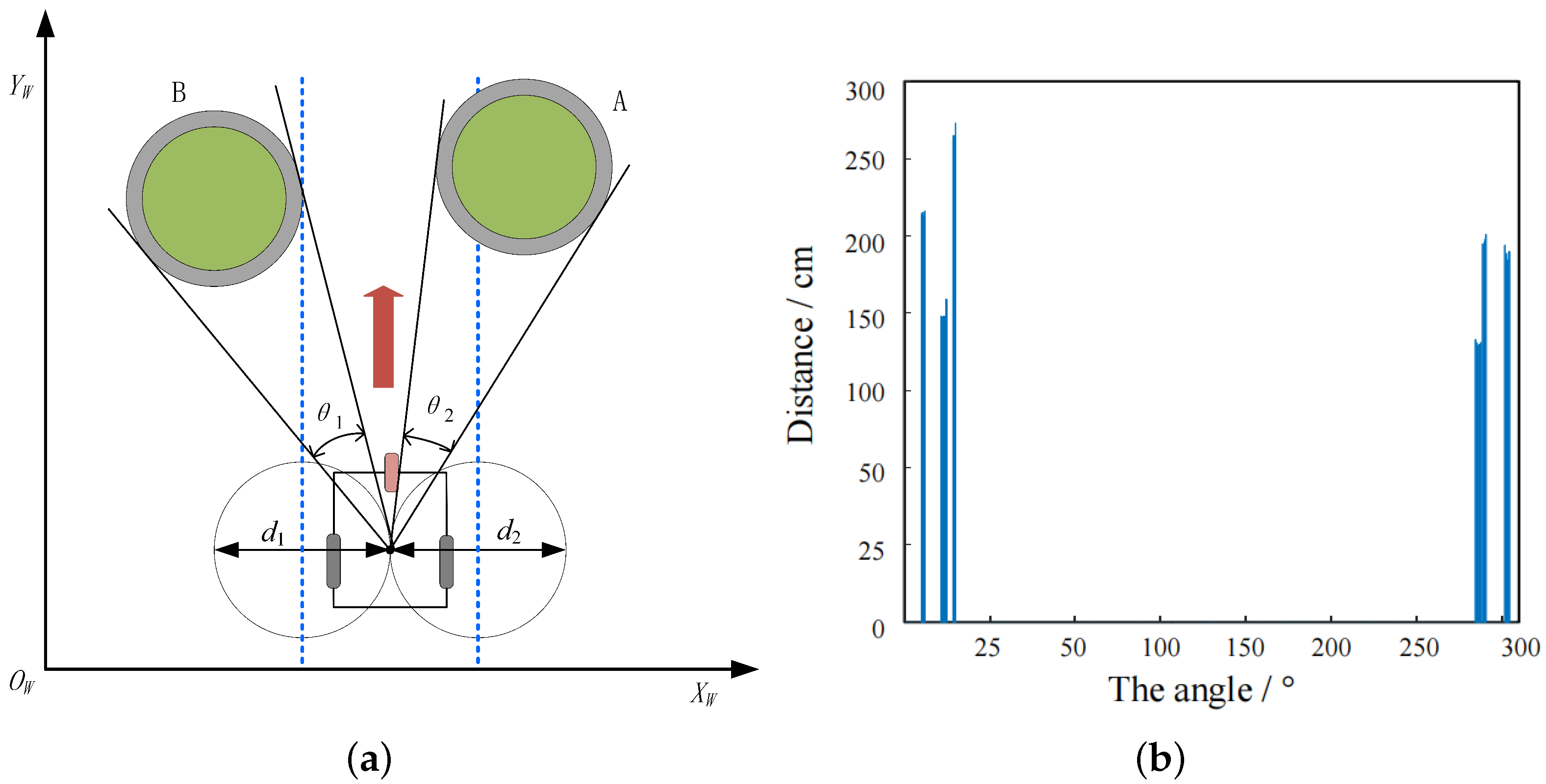
- An improved density-based fast clustering algorithm is proposed, combined with a convex hull algorithm and rotating jamming algorithm to analyze obstacle information, and an obstacle avoidance path and heading control method based on the dangerous area of obstacles is developed. The feasibility of low-cost obstacle avoidance using LiDAR in agricultural robots is realized.
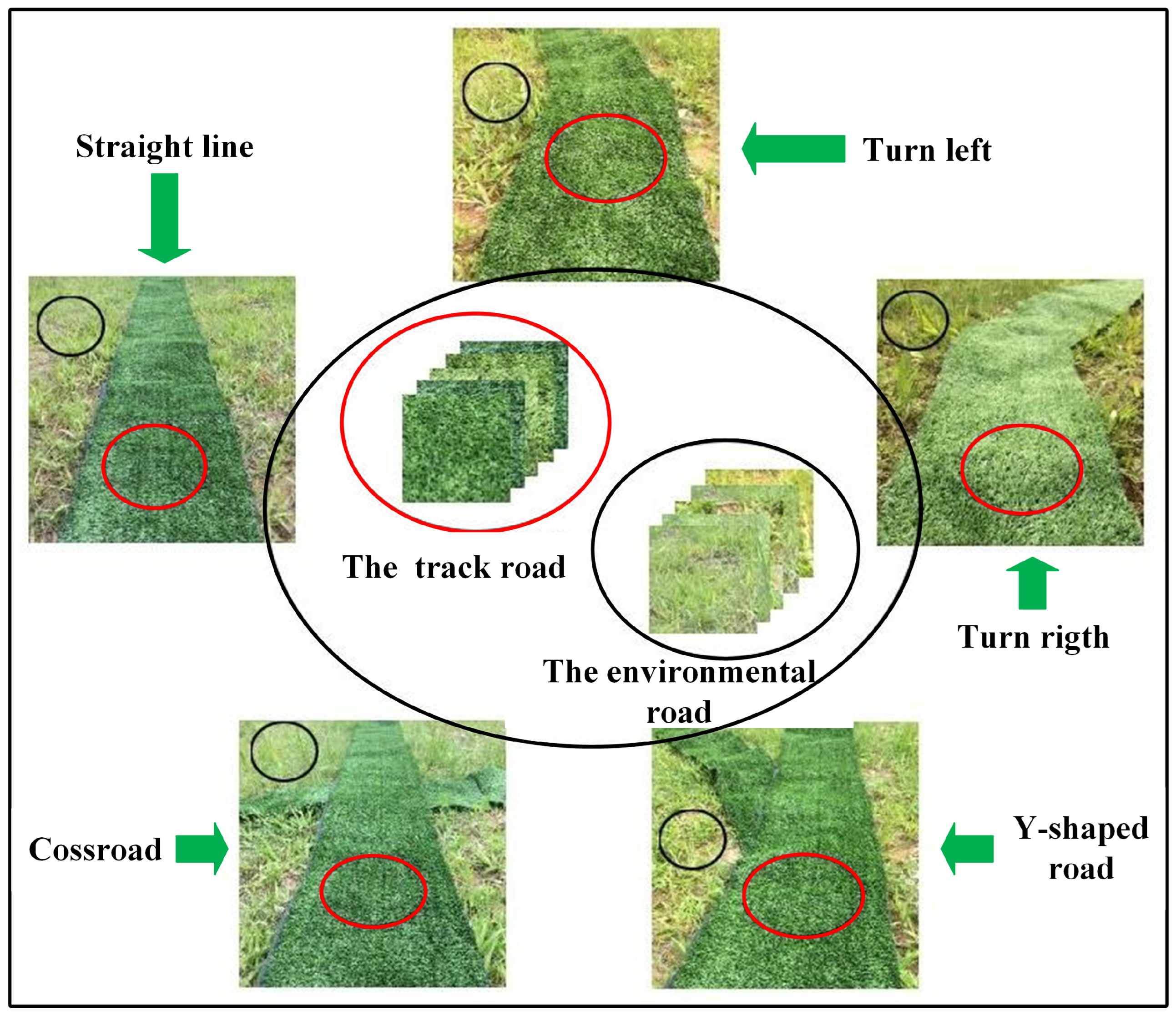
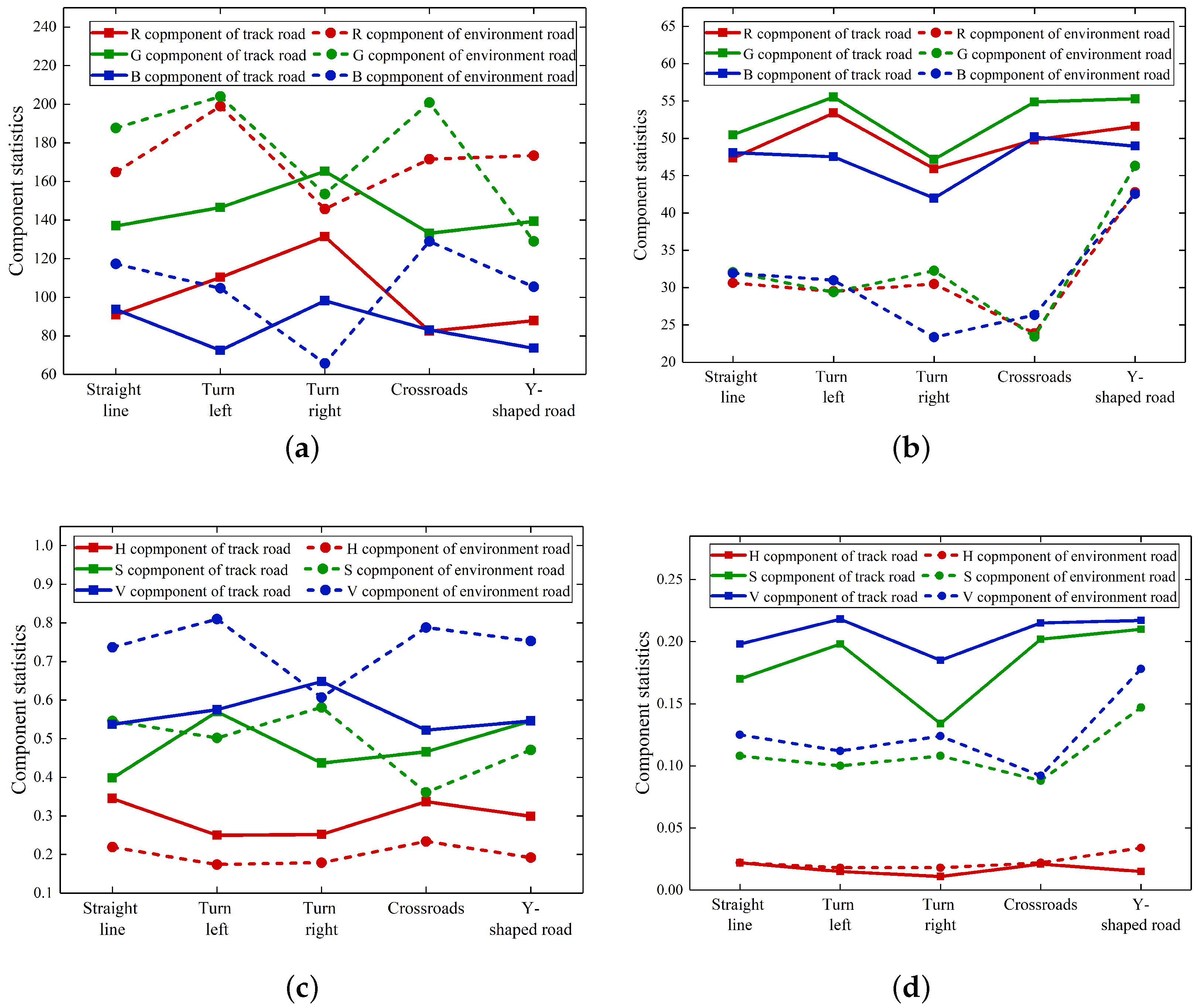
- By analyzing the color space information of the orchard environment road and track road images, a robot track navigation route and control method based on image features were proposed. A vision camera was used to assist agricultural robots in navigation, and the orchard path feature recognition task was preliminarily solved.
- An agricultural robot navigation and obstacle avoidance system based on a vision camera and LiDAR is designed, which makes up for the shortcomings of poor robustness and easy to be disturbed by the environment of a single sensor, and realizes the stable work of agricultural robots working in the environment rejected by GNSS.
2. Preliminaries
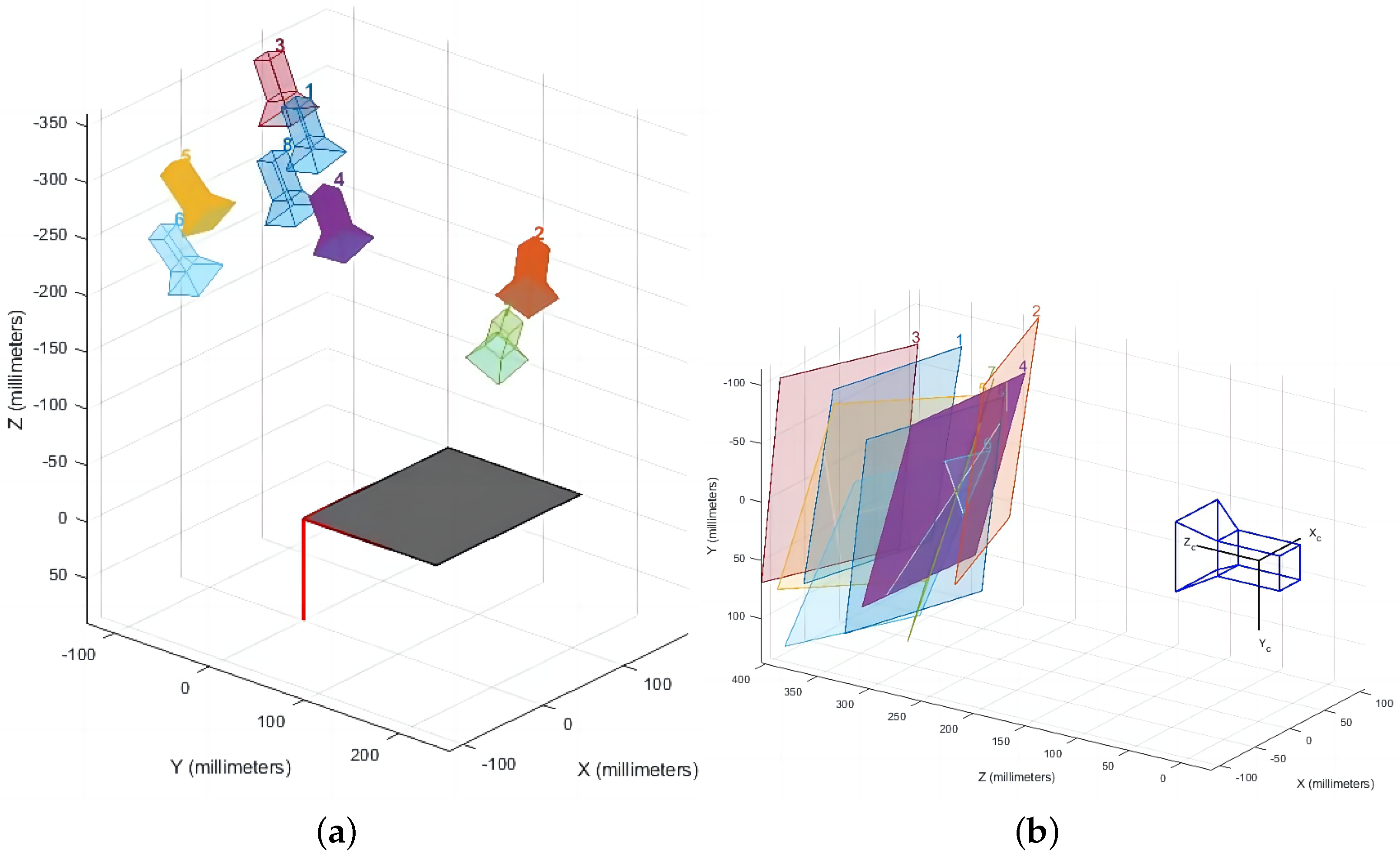
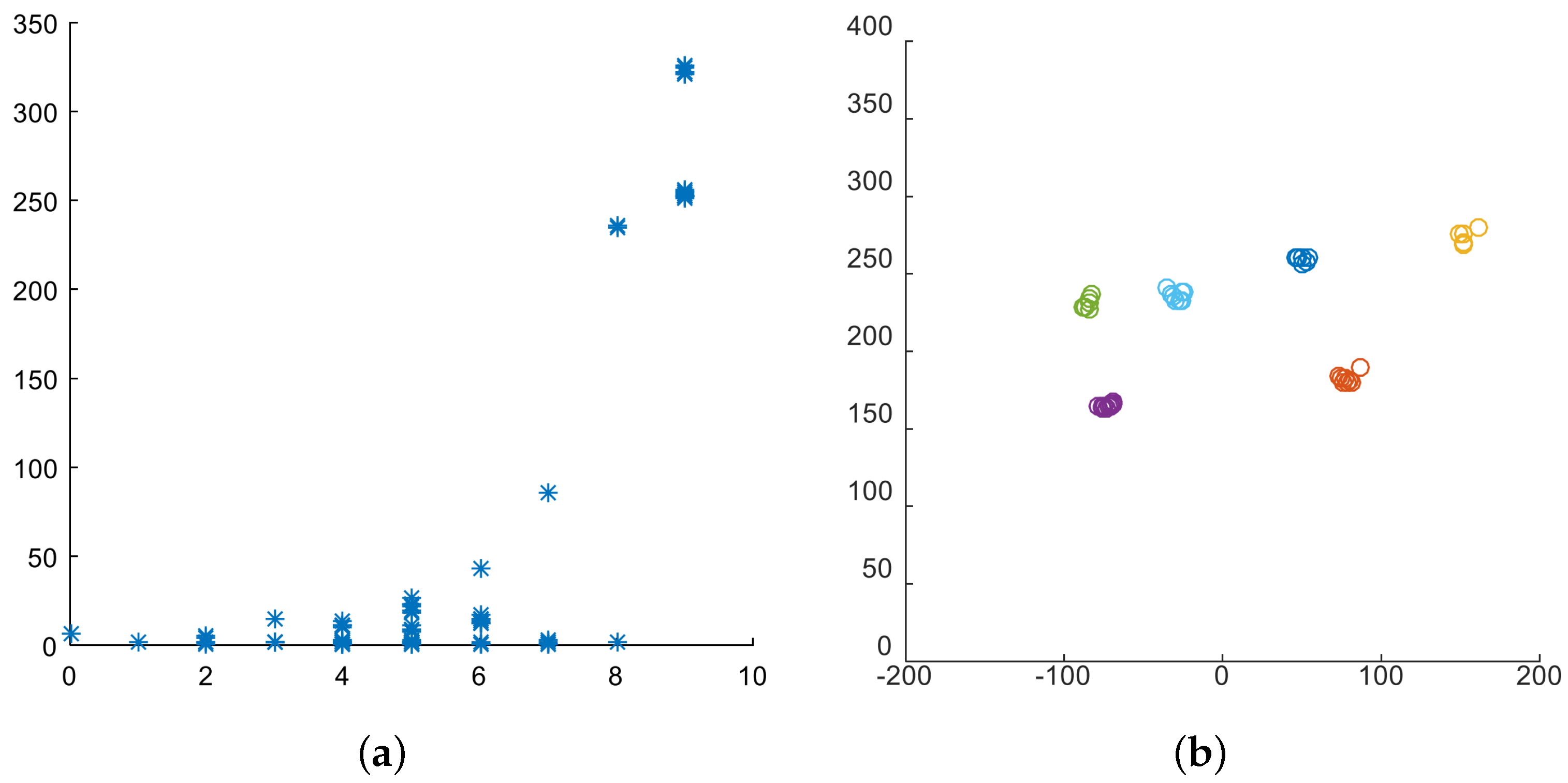
2.1. LiDAR Calibration and Filtering Processing
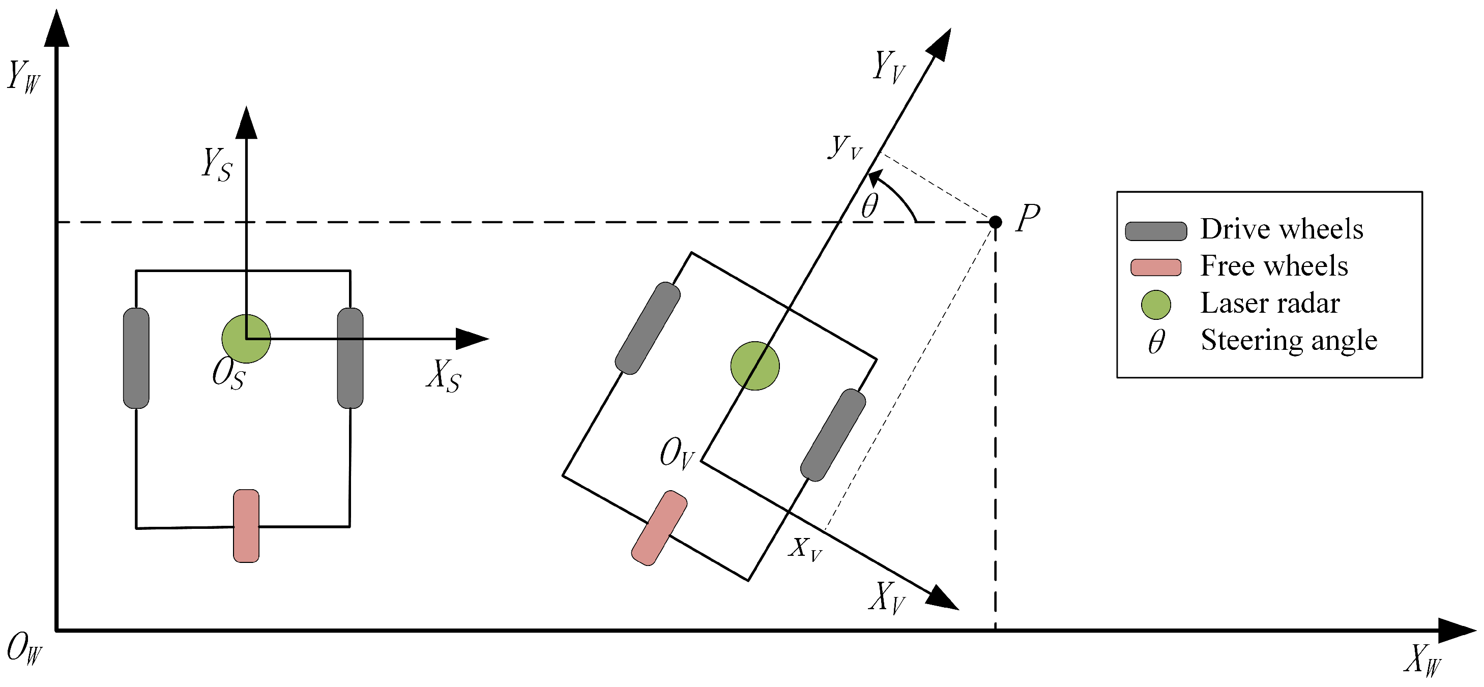
2.2. Camera Visualization and Parameter Calibration
3. Obstacle Avoidance System and Algorithm Implementation
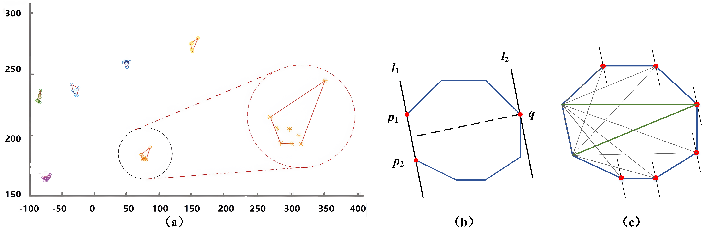
3.1. Improved Clustering Algorithm of Obstacle Point Cloud Information
3.2. The Fusion of Convex Hull Algorithm and Rotary Jamming Algorithm
3.3. Path Planning and Heading Control of the Robot
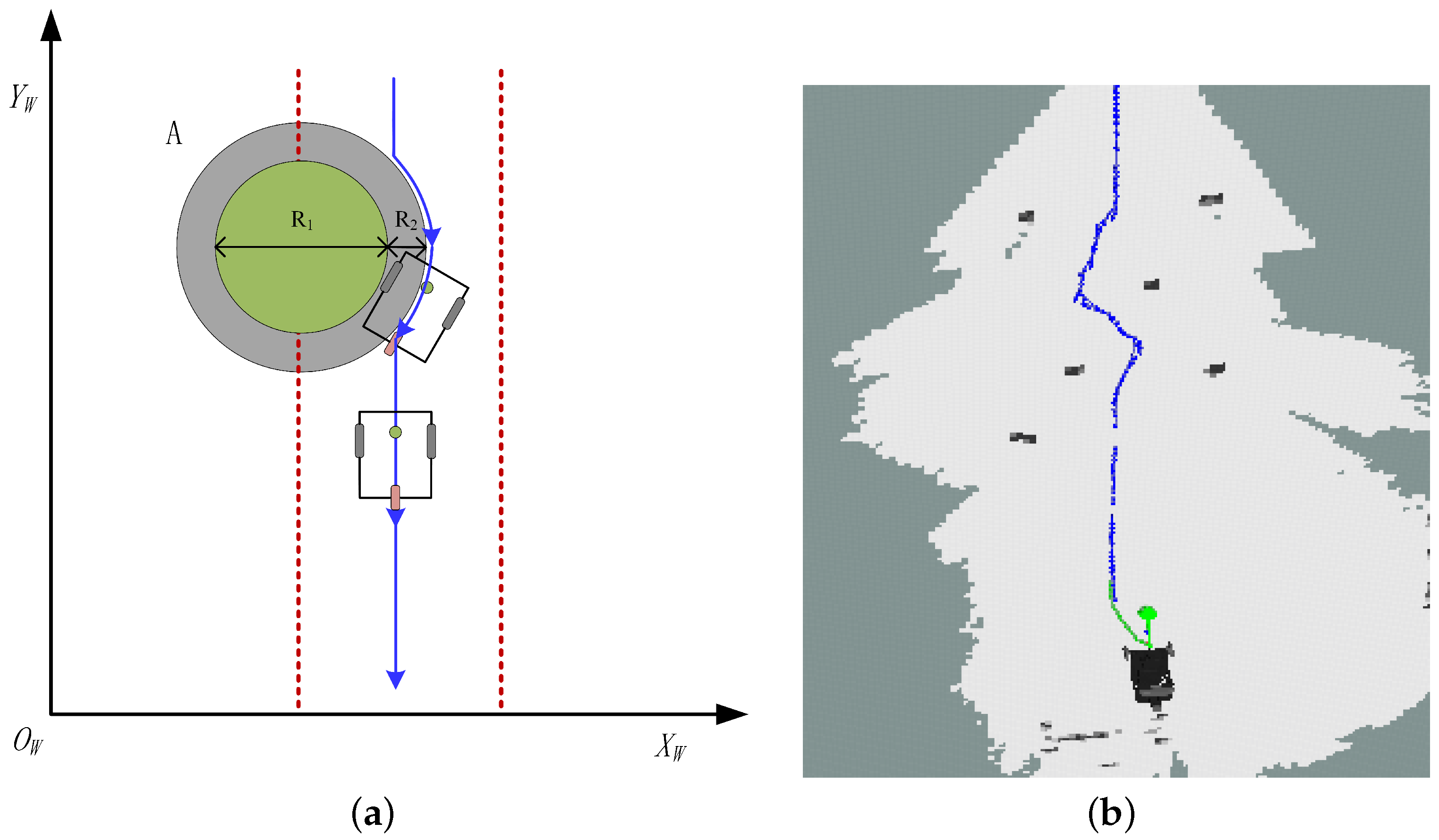
3.3.1. Obstacle Avoidance Path Planning
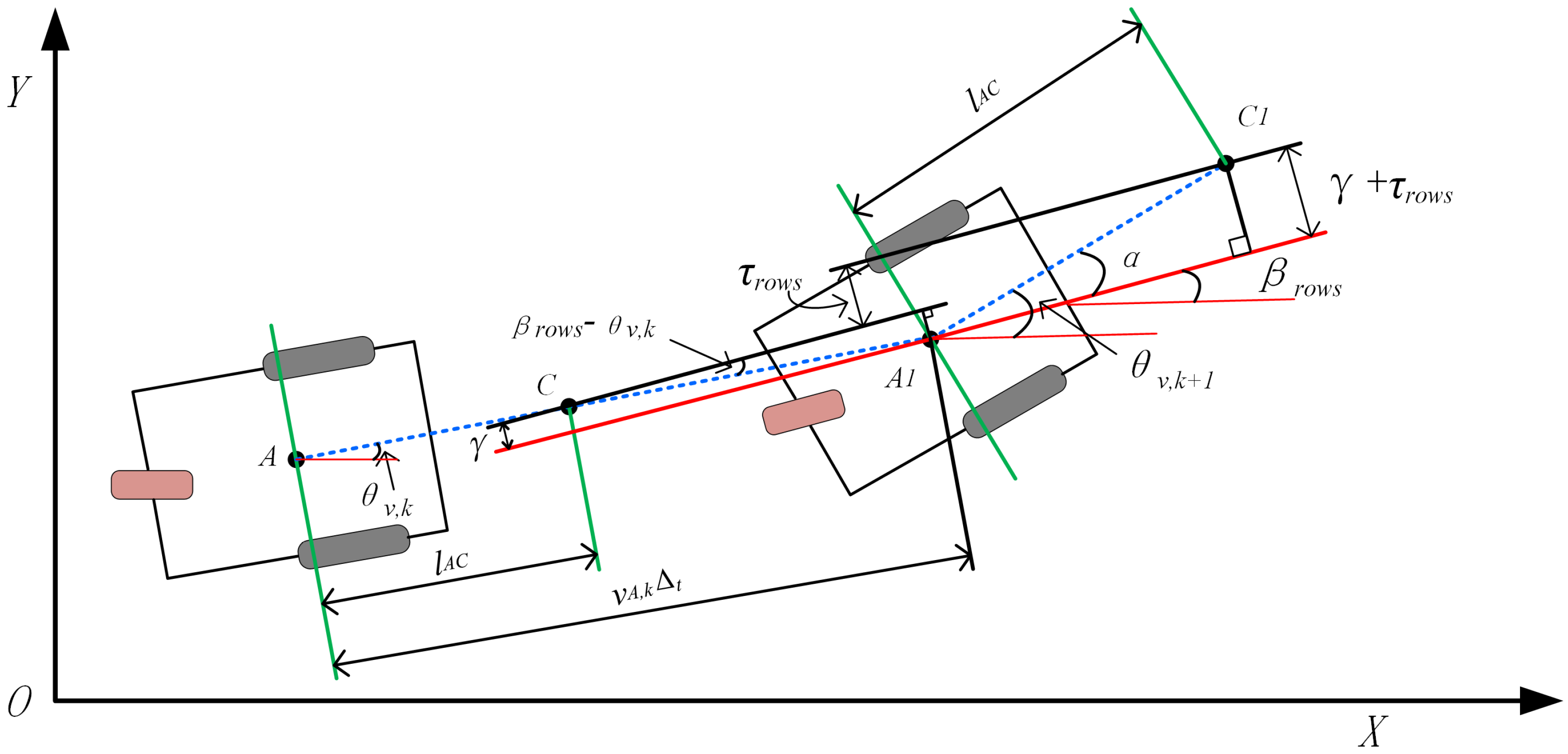
3.3.2. Heading Control of the Robot
4. Visual Navigation System
4.1. Color Space of Track Road and Environment Road
4.2. The Processing of Road Image of Guiding Trajectory
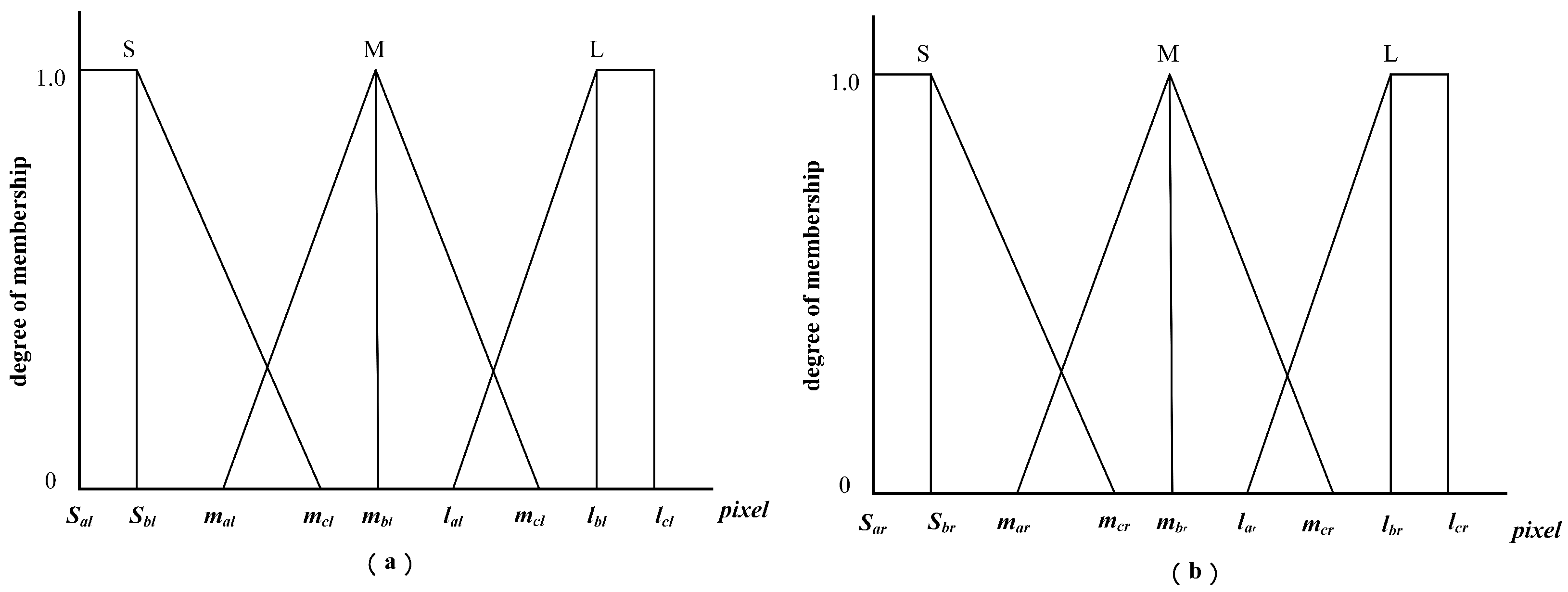
4.3. Fuzzy Logic Vision Control System Based on Visual Pixels
5. Experimental Test Results of Autonomous Robot
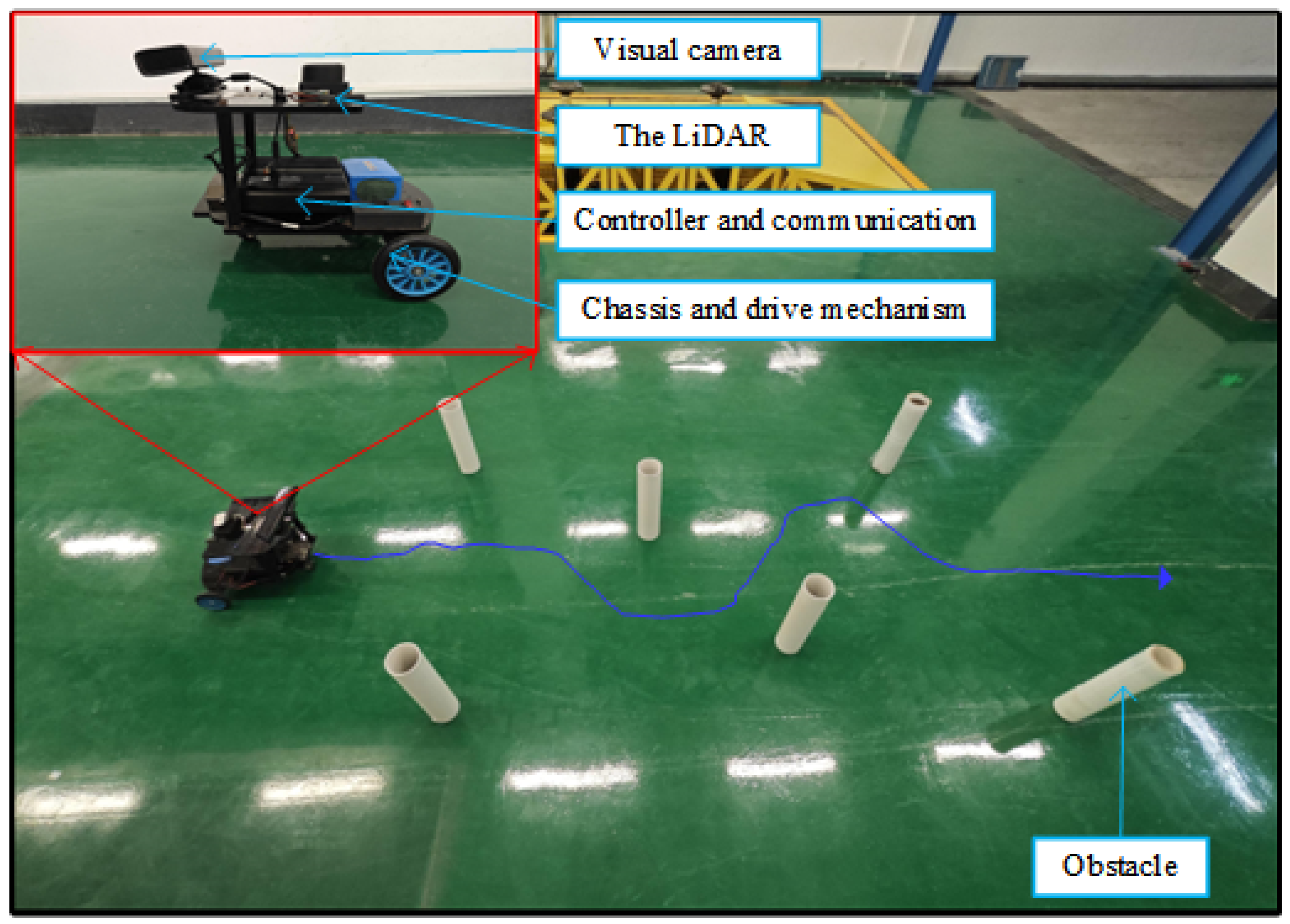
5.1. System Composition
5.2. Test of Obstacle Avoidance System
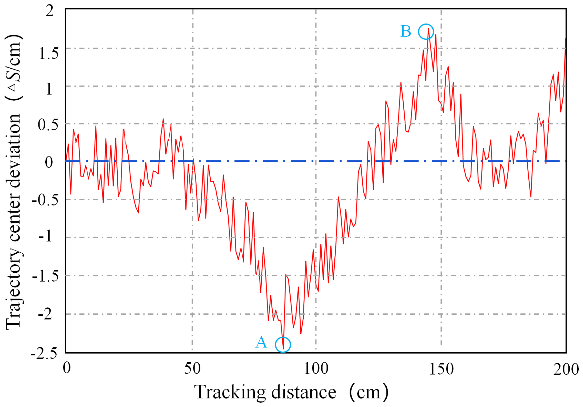
5.3. Test of Visual Guidance System
6. Conclusions and Future Works
Author Contributions
Funding
Data Availability Statement
Conflicts of Interest
References
- Albiero, D.; Garcia, A.P.; Umezu, C.K.; de Paulo, R.L. Swarm robots in mechanized agricultural operations: A review about challenges for research. Comput. Electron. Agric. 2022, 193, 106608. [Google Scholar] [CrossRef]
- Jin, Y.; Liu, J.; Xu, Z.; Yuan, S.; Li, P.; Wang, J. Development status and trend of agricultural robot technology. Int. J. Agric. Biol. Eng. 2021, 14, 1–19. [Google Scholar] [CrossRef]
- Li, J.; Li, J.; Zhao, X.; Su, X.; Wu, W. Lightweight detection networks for tea bud on complex agricultural environment via improved YOLO v4. Comput. Electron. Agric. 2023, 211, 107955. [Google Scholar] [CrossRef]
- Sparrow, R.; Howard, M. Robots in agriculture: Prospects, impacts, ethics, and policy. Precis. Agric. 2021, 22, 818–833. [Google Scholar] [CrossRef]
- Ju, C.; Kim, J.; Seol, J.; Son, H.I. A review on multirobot systems in agriculture. Comput. Electron. Agric. 2022, 202, 107336. [Google Scholar] [CrossRef]
- Bechar, A.; Vigneault, C. Agricultural robots for field operations: Concepts and components. Biosyst. Eng. 2016, 149, 94–111. [Google Scholar] [CrossRef]
- Liu, X.; Wang, J.; Li, J. URTSegNet: A real-time segmentation network of unstructured road at night based on thermal infrared images for autonomous robot system. Control. Eng. Pract. 2023, 137, 105560. [Google Scholar] [CrossRef]
- Dutta, A.; Roy, S.; Kreidl, O.P.; Bölöni, L. Multi-robot information gathering for precision agriculture: Current state, scope, and challenges. IEEE Access 2021, 9, 161416–161430. [Google Scholar] [CrossRef]
- Malavazi, F.B.; Guyonneau, R.; Fasquel, J.B.; Lagrange, S.; Mercier, F. LiDAR-only based navigation algorithm for an autonomous agricultural robot. Comput. Electron. Agric. 2018, 154, 71–79. [Google Scholar] [CrossRef]
- Rouveure, R.; Faure, P.; Monod, M.O. PELICAN: Panoramic millimeter-wave radar for perception in mobile robotics applications, Part 1: Principles of FMCW radar and of 2D image construction. Robot. Auton. Syst. 2016, 81, 1–16. [Google Scholar] [CrossRef]
- Ball, D.; Upcroft, B.; Wyeth, G.; Corke, P.; English, A.; Ross, P.; Patten, T.; Fitch, R.; Sukkarieh, S.; Bate, A. Vision-based obstacle detection and navigation for an agricultural robot. J. Field Robot. 2016, 33, 1107–1130. [Google Scholar] [CrossRef]
- Santos, L.C.; Santos, F.N.; Valente, A.; Sobreira, H.; Sarmento, J.; Petry, M. Collision avoidance considering iterative Bézier based approach for steep slope terrains. IEEE Access 2022, 10, 25005–25015. [Google Scholar] [CrossRef]
- Monarca, D.; Rossi, P.; Alemanno, R.; Cossio, F.; Nepa, P.; Motroni, A.; Gabbrielli, R.; Pirozzi, M.; Console, C.; Cecchini, M. Autonomous Vehicles Management in Agriculture with Bluetooth Low Energy (BLE) and Passive Radio Frequency Identification (RFID) for Obstacle Avoidance. Sustainability 2022, 14, 9393. [Google Scholar] [CrossRef]
- Blok, P.; Suh, H.; van Boheemen, K.; Kim, H.J.; Gookhwan, K. Autonomous in-row navigation of an orchard robot with a 2D LIDAR scanner and particle filter with a laser-beam model. J. Inst. Control. Robot. Syst. 2018, 24, 726–735. [Google Scholar] [CrossRef]
- Gao, X.; Li, J.; Fan, L.; Zhou, Q.; Yin, K.; Wang, J.; Song, C.; Huang, L.; Wang, Z. Review of wheeled mobile robots’ navigation problems and application prospects in agriculture. IEEE Access 2018, 6, 49248–49268. [Google Scholar] [CrossRef]
- Wang, T.; Chen, B.; Zhang, Z.; Li, H.; Zhang, M. Applications of machine vision in agricultural robot navigation: A review. Comput. Electron. Agric. 2022, 198, 107085. [Google Scholar] [CrossRef]
- Durand-Petiteville, A.; Le Flecher, E.; Cadenat, V.; Sentenac, T.; Vougioukas, S. Tree detection with low-cost three-dimensional sensors for autonomous navigation in orchards. IEEE Robot. Autom. Lett. 2018, 3, 3876–3883. [Google Scholar] [CrossRef]
- Higuti, V.A.; Velasquez, A.E.; Magalhaes, D.V.; Becker, M.; Chowdhary, G. Under canopy light detection and ranging-based autonomous navigation. J. Field Robot. 2019, 36, 547–567. [Google Scholar] [CrossRef]
- Guyonneau, R.; Mercier, F.; Oliveira, G.F. LiDAR-Only Crop Navigation for Symmetrical Robot. Sensors 2022, 22, 8918. [Google Scholar] [CrossRef]
- Nehme, H.; Aubry, C.; Solatges, T.; Savatier, X.; Rossi, R.; Boutteau, R. Lidar-based structure tracking for agricultural robots: Application to autonomous navigation in vineyards. J. Intell. Robot. Syst. 2021, 103, 61. [Google Scholar] [CrossRef]
- Hiremath, S.A.; Van Der Heijden, G.W.; Van Evert, F.K.; Stein, A.; Ter Braak, C.J. Laser range finder model for autonomous navigation of a robot in a maize field using a particle filter. Comput. Electron. Agric. 2014, 100, 41–50. [Google Scholar] [CrossRef]
- Zhao, R.M.; Zhu, Z.; Chen, J.N.; Yu, T.J.; Ma, J.J.; Fan, G.S.; Wu, M.; Huang, P.C. Rapid development methodology of agricultural robot navigation system working in GNSS-denied environment. Adv. Manuf. 2023, 11, 601–617. [Google Scholar] [CrossRef]
- Winterhalter, W.; Fleckenstein, F.; Dornhege, C.; Burgard, W. Localization for precision navigation in agricultural fields—Beyond crop row following. J. Field Robot. 2021, 38, 429–451. [Google Scholar] [CrossRef]
- Chen, W.; Sun, J.; Li, W.; Zhao, D. A real-time multi-constraints obstacle avoidance method using LiDAR. J. Intell. Fuzzy Syst. 2020, 39, 119–131. [Google Scholar] [CrossRef]
- Lenac, K.; Kitanov, A.; Cupec, R.; Petrović, I. Fast planar surface 3D SLAM using LIDAR. Robot. Auton. Syst. 2017, 92, 197–220. [Google Scholar] [CrossRef]
- Park, J.; Cho, N. Collision Avoidance of Hexacopter UAV Based on LiDAR Data in Dynamic Environment. Remote Sens. 2020, 12, 975. [Google Scholar] [CrossRef]
- Li, J.; Wang, J.; Peng, H.; Hu, Y.; Su, H. Fuzzy-Torque Approximation-Enhanced Sliding Mode Control for Lateral Stability of Mobile Robot. IEEE Trans. Syst. Man Cybern. 2022, 52, 2491–2500. [Google Scholar]
- Wang, D.; Chen, X.; Liu, J.; Liu, Z.; Zheng, F.; Zhao, L.; Li, J.; Mi, X. Fast Positioning Model and Systematic Error Calibration of Chang’E-3 Obstacle Avoidance Lidar for Soft Landing. Sensors 2022, 22, 7366. [Google Scholar] [CrossRef]
- Kim, J.S.; Lee, D.H.; Kim, D.W.; Park, H.; Paik, K.J.; Kim, S. A numerical and experimental study on the obstacle collision avoidance system using a 2D LiDAR sensor for an autonomous surface vehicle. Ocean Eng. 2022, 257, 111508. [Google Scholar] [CrossRef]
- Asvadi, A.; Premebida, C.; Peixoto, P.; Nunes, U. 3D Lidar-based static and moving obstacle detection in driving environments: An approach based on voxels and multi-region ground planes. Robot. Auton. Syst. 2016, 83, 299–311. [Google Scholar] [CrossRef]
- Baek, J.; Noh, G.; Seo, J. Robotic Camera Calibration to Maintain Consistent Percision of 3D Trackers. Int. J. Precis. Eng. Manuf. 2021, 22, 1853–1860. [Google Scholar] [CrossRef]
- Li, J.; Dai, Y.; Su, X.; Wu, W. Efficient Dual-Branch Bottleneck Networks of Semantic Segmentation Based on CCD Camera. Remote Sens. 2022, 14, 3925. [Google Scholar] [CrossRef]
- Dong, H.; Weng, C.Y.; Guo, C.; Yu, H.; Chen, I.M. Real-time avoidance strategy of dynamic obstacles via half model-free detection and tracking with 2d lidar for mobile robots. IEEE/ASME Trans. Mechatron. 2020, 26, 2215–2225. [Google Scholar] [CrossRef]
- Choi, Y.; Jimenez, H.; Mavris, D.N. Two-layer obstacle collision avoidance with machine learning for more energy-efficient unmanned aircraft trajectories. Robot. Auton. Syst. 2017, 98, 158–173. [Google Scholar] [CrossRef]
- Gao, F.; Li, C.; Zhang, B. A dynamic clustering algorithm for LiDAR obstacle detection of autonomous driving system. IEEE Sens. J. 2021, 21, 25922–25930. [Google Scholar] [CrossRef]
- Jin, X.Z.; Zhao, Y.X.; Wang, H.; Zhao, Z.; Dong, X.P. Adaptive fault-tolerant control of mobile robots with actuator faults and unknown parameters. IET Control. Theory Appl. 2019, 13, 1665–1672. [Google Scholar] [CrossRef]
- Zhang, H.D.; Liu, S.B.; Lei, Q.J.; He, Y.; Yang, Y.; Bai, Y. Robot programming by demonstration: A novel system for robot trajectory programming based on robot operating system. Adv. Manuf. 2020, 8, 216–229. [Google Scholar] [CrossRef]
- Raikwar, S.; Fehrmann, J.; Herlitzius, T. Navigation and control development for a four-wheel-steered mobile orchard robot using model-based design. Comput. Electron. Agric. 2022, 202, 107410. [Google Scholar] [CrossRef]
- Gheisarnejad, M.; Khooban, M.H. Supervised Control Strategy in Trajectory Tracking for a Wheeled Mobile Robot. IET Collab. Intell. Manuf. 2019, 1, 3–9. [Google Scholar] [CrossRef]
- Hess, W.; Kohler, D.; Rapp, H.; Andor, D. Real-time loop closure in 2D LIDAR SLAM. In Proceedings of the 2016 IEEE International Conference on Robotics and Automation (ICRA), Stockholm, Sweden, 16–21 May 2016; pp. 1271–1278. [Google Scholar]
- Yang, C.; Chen, C.; Wang, N.; Ju, Z.; Fu, J.; Wang, M. Biologically inspired motion modeling and neural control for robot learning from demonstrations. IEEE Trans. Cogn. Dev. Syst. 2018, 11, 281–291. [Google Scholar]
- Wu, J.; Wang, H.; Zhang, M.; Yu, Y. On obstacle avoidance path planning in unknown 3D environments: A fluid-based framework. ISA Trans. 2021, 111, 249–264. [Google Scholar] [CrossRef] [PubMed]
- Liu, C.; Tomizuka, M. Real time trajectory optimization for nonlinear robotic systems: Relaxation and convexification. Syst. Control. Lett. 2017, 108, 56–63. [Google Scholar] [CrossRef]
- Zhang, Q.; Chen, M.S.; Li, B. A visual navigation algorithm for paddy field weeding robot based on image understanding. Comput. Electron. Agric. 2017, 143, 66–78. [Google Scholar] [CrossRef]
- Liu, Q.; Yang, F.; Pu, Y.; Zhang, M.; Pan, G. Segmentation of farmland obstacle images based on intuitionistic fuzzy divergence. J. Intell. Fuzzy Syst. 2016, 31, 163–172. [Google Scholar] [CrossRef]
- Liu, M.; Ren, D.; Sun, H.; Yang, S.X.; Shao, P. Orchard Areas Segmentation in Remote Sensing Images via Class Feature Aggregate Discriminator. IEEE Geosci. Remote Sens. Lett. 2022, 19, 1–5. [Google Scholar] [CrossRef]
- Mills, L.; Flemmer, R.; Flemmer, C.; Bakker, H. Prediction of kiwifruit orchard characteristics from satellite images. Precis. Agric. 2019, 20, 911–925. [Google Scholar] [CrossRef]
- Liu, S.; Wang, X.; Li, S.; Chen, X.; Zhang, X. Obstacle avoidance for orchard vehicle trinocular vision system based on coupling of geometric constraint and virtual force field method. Expert Syst. Appl. 2022, 190, 116216. [Google Scholar] [CrossRef]
- Begnini, M.; Bertol, D.W.; Martins, N.A. A robust adaptive fuzzy variable structure tracking control for the wheeled mobile robot: Simulation and experimental results. Control. Eng. Pract. 2017, 64, 27–43. [Google Scholar] [CrossRef]
- Zhang, F.; Zhang, W.; Luo, X.; Zhang, Z.; Lu, Y.; Wang, B. Developing an ioT-enabled cloud management platform for agricultural machinery equipped with automatic navigation systems. Agriculture 2022, 12(2), 310. [Google Scholar] [CrossRef]
- Zhao, Z.; Zhang, Y.; Long, L.; Lu, Z.; Shi, J. Efficient and adaptive lidar visual inertial odometry for agricultural unmanned ground vehicle. Int. J. Adv. Robot. Syst. 2022, 19, 17298806221094925. [Google Scholar] [CrossRef]


| Steps | Content |
|---|---|
| Input | The remaining points in X(); |
| Output | Convex hull results |
| 1 | Sort () by its polar angle counterclockwise to ; |
| 2 | If several points have the same polar angle; |
| 3 | Then, remove the rest of the points; |
| 4 | Then, leaving only the point farthest from ; |
| 5 | PUSH(, S); |
| 6 | PUSH(, S); |
| 7 | PUSH(, S); |
| 8 | for i←3 to m; |
| 10 | Call the function: TOP(S) and form a non-left-turn do; |
| 11 | Call function NEXT-TOP(S) and return the following point; |
| 12 | POP(S); |
| 13 | PUSH(, S); |
| 14 | end for |
| 15 | return S |
| Steps | Content |
|---|---|
| Input | Point coordinates of the polygon (); |
| Output | Maximum diameter () and the “heel point pair” |
| 1 | ← min(); |
| 2 | ← max(), calculate the endpoints and ; |
| 3 | n← 1; |
| 4 | While n < N do; |
| 5 | ; |
| 6 | ← (), calculate the distance between and ; |
| 7 | Design two horizontal tangents and through and ; |
| 8 | Rotate and until they coincide with the other side of the polygon; |
| 9 | ← max(), Create new heel points; |
| 10 | Calculate the new distance and compare the sizes; |
| 11 | End |
| Number | PCLeft | PCRight | ||
|---|---|---|---|---|
| 1 | Small | Small | 90 | |
| 2 | Small | Medium | 67 | |
| 3 | Small | Large | 45 | |
| 4 | Medium | Small | 112 | |
| 5 | Medium | Medium | 90 | |
| 6 | Medium | Large | 67 | |
| 7 | Large | Small | 135 | |
| 8 | Large | Medium | 112 | |
| 9 | Large | Large | 60 |
| Sampling Rate (S·s) | The Length of Robot (/cm) | The Width of Robot (/cm) | The Width of Trajectory (/cm) | The Average Rotational Speed of Robot (/r·min) |
|---|---|---|---|---|
| 10 | 30 | 45 | 35 | 20 |
Disclaimer/Publisher’s Note: The statements, opinions and data contained in all publications are solely those of the individual author(s) and contributor(s) and not of MDPI and/or the editor(s). MDPI and/or the editor(s) disclaim responsibility for any injury to people or property resulting from any ideas, methods, instructions or products referred to in the content. |
© 2023 by the authors. Licensee MDPI, Basel, Switzerland. This article is an open access article distributed under the terms and conditions of the Creative Commons Attribution (CC BY) license (https://creativecommons.org/licenses/by/4.0/).
Share and Cite
Han, C.; Wu, W.; Luo, X.; Li, J. Visual Navigation and Obstacle Avoidance Control for Agricultural Robots via LiDAR and Camera. Remote Sens. 2023, 15, 5402. https://doi.org/10.3390/rs15225402
Han C, Wu W, Luo X, Li J. Visual Navigation and Obstacle Avoidance Control for Agricultural Robots via LiDAR and Camera. Remote Sensing. 2023; 15(22):5402. https://doi.org/10.3390/rs15225402
Chicago/Turabian StyleHan, Chongyang, Weibin Wu, Xiwen Luo, and Jiehao Li. 2023. "Visual Navigation and Obstacle Avoidance Control for Agricultural Robots via LiDAR and Camera" Remote Sensing 15, no. 22: 5402. https://doi.org/10.3390/rs15225402
APA StyleHan, C., Wu, W., Luo, X., & Li, J. (2023). Visual Navigation and Obstacle Avoidance Control for Agricultural Robots via LiDAR and Camera. Remote Sensing, 15(22), 5402. https://doi.org/10.3390/rs15225402