An Observation of Precipitation during Cooling with Ka-Band Cloud Radar in Wuhan, China

Abstract

Exploiting their sensitivity to cloud droplets and small raindrops, Ka-band cloud radar observations are used to investigate weak stratiform precipitation over Wuhan during cooling on 16–17 February 2022. During cooling, the surface temperature drops by about 8 °C with the lowest value less than 0 °C because of the strong cold air from the north. The cold air lifts the warm and humid air transported by the southeasterly and southwesterly winds, causing thick stratiform clouds and persistent weak precipitation. The Ka-band radar captures the full process of stratiform cloud occurrence; light rain and then mixed rain and snow; and the characteristics of clouds and precipitation at each stage due to its fine sensitivity to small hydrometeors, whereas the reanalysis data alone cannot capture the transition to the mixed rain and snow regime, which can cause dangerous freezing rain or sleet on the ground. Hence, a detailed analysis of cooling and cold surges and their hazards to society, and their reproduction in numerical predictions, needs to use high-sensitivity radar data as much as possible.

1. Introduction

Clouds and precipitation are an important phase of the water cycle and critical to understanding the radiation budget and regional and global climatic variabilities [1,2,3]. There are different types of atmospheric precipitation, which depend on the updraft, water vapor supply, and macro and micro physical features of clouds. In terms of the causes and forms of rising air movement, precipitation can generally be divided into convective precipitation, topographic precipitation, typhoon precipitation, and frontal precipitation [4,5,6]. When a front approaches, warm moist air climbs either actively or passively; thus, water vapor condenses as the temperature of the rising air drops, leading to cloud formation and precipitation. Frontal rain usually lasts for a longer duration relative to convective rain, whereas its intensity is smaller compared with convective rain because stratiform clouds formed during the frontal process have a slower rise [7,8]. When stratiform clouds are thick, they can provide long collision distances for cloud droplets and reduce evaporation from falling raindrops, which is conducive to the formation of precipitation. Frontal precipitation and convective precipitation are two common forms of precipitation in the middle and lower reaches of the Changjiang River in China.

Stratiform rainfall is one of the most frequent forms of precipitation in global weather patterns [9,10,11,12,13]. In stratiform precipitation, there is an evident feature of a high-intensity echo band that occurs below the 0 °C isotherm level, which is identified as the localized maxima in the radar reflectivity factor [14,15,16], called the bright band. Thus, stratiform precipitation is also referred to as bright band precipitation [17]. The bright band is attributed to the variation in the scattering properties of precipitation particles due to the melting of descending snowflakes and ices as they pass through the 0 °C level [10,15,18,19]. Since the dielectric constant of water is approximately five times that of ice [20,21], the dielectric constant of hydrometeors increases rapidly in the melting layer, while the raindrop concentrations decrease owing to the enhanced fall velocities of melting snowflakes and ices toward the end of the melting process, causing the bright band in the reflectivity factor [22,23]. In addition to the changes in reflectivity and fall speed, the depolarization effect in the melting layer can be observed via polarization radar and lidar when non-spherical snowflakes and ices melt into near-spherical raindrops [24,25,26,27,28]. Microphysical processes in the melting layer, such as the melting, merging, falling, and breaking of hydrometeors, play an important role in exploring rainfall mechanisms and quantitatively assessing rainfall [16,29,30]. Hence, the characteristics of bright bands and their implication in microphysical processes in the melting layer have been attracting considerable attention from observational, theoretical, and modeling studies since the advent of radar meteorology [22,31,32,33].

An S-band radar located in southern England observed the different vertical profiles of reflectivity for two precipitation types. The bright band could not be observed in areas of strong convection rainfall because of the intense vertical mixing of high-density graupel or soft hail by convection, but could be observed in areas of stratiform precipitation [34]. Triple-wavelength Doppler radar measurements of rain showers showed that, in contrast to the prevalent S-band radar bright band dominated by the Rayleigh dielectric scattering effects, the bright band is intermittent in Ka-band radar observation and unsharp in W-band radar measurement owing to the dominance of the non-Rayleigh scattering effect [35], implying that the presence of the bright band is related to the radar wavelength. By combining weather radar and millimeter wave radar observations, it was noted that as the precipitation intensity increases from drizzle to heavy rainfall, the peak and thickness of the bright band are enhanced, but its height descends [23,36]. Nevertheless, due to the short operating wavelength, the millimeter-wave radar has a fine sensitivity to cloud droplets and tiny raindrops, and can obtain the information of non-precipitation and weak-precipitation cloud tops; thus, it is suitable for detecting microphysical processes in weak precipitation where attenuation is much weaker than in heavy rainfall [36,37].

Cooling is a frequent event at mid-latitudes in the Northern Hemisphere from late winter to early spring, which can result in serious threats to human health, agriculture and transportation, and economic loss [38,39]. As strong cold events, cold surges, defined generally as intense cooling that causes a temperature drop of more than 10 °C in 24 h with a minimum temperature lower than 5 °C, showed a growing trend in the context of global warming [40]. As cold northerly winds blow from high latitudes, the temperature drops rapidly, followed by precipitation, and precipitation often transitions from rain to a variety of ice-based forms, including sleet, snow, ice particles, and freezing rain. In this study, we present a cooling process over Wuhan in winter, which leads to thick stratiform clouds and light precipitation. Thus, this scenario is ideal for a Ka-band radar to capture the cloud formation and precipitation processes. In the next section, the Ka-band radar and data used are described briefly. In Section 3, the processes of cooling and precipitation are presented by combining the radar and radiosonde observations and reanalysis data, and the features of light rain and mixed rain and snow are discussed in detail. The atmospheric conditions in stratiform precipitation are analyzed in Section 4. Section 5 provides a summary.

2. Radar and Data

The millimeter cloud radar (MMCR) is situated at the Atmospheric Remote Sensing Observatory (ARSO) in Wuhan University (30.5°N, 114.4°E, 40 m above sea level). As an inland megacity in central China, Wuhan City, located in the east of the Jianghan plain, is dominated by a subtropical monsoon humid climate. In summer, rain and even rainstorms frequently occur due to lots of water vapor transported by monsoons. In winter, because of the inflow of cold air to the south, the temperature can evidently drop, and the cooling process often leads to rain and snow.

2.1. Ka-Band MMCR

The MMCR established by the ARSO of Wuhan University is a Ka-band dual-polarization frequency-modulated continuous wave (FMCW) Doppler radar. The two transmitters with a mean power of 50 W transmit mutually orthogonal polarized continuous-wave signals at an operating frequency of 35.035 GHz through a 0.38° wide beam formed by a Cassegrain antenna with a 1.5 m diameter, and echoes backscattered by cloud particles and raindrops are received by the other same Cassegrain antenna. The two polarized echo signals are sent to the corresponding signal processing systems, respectively, and then the parameters, such as the reflectivity factor (Z), Doppler velocity (V), Doppler spectrum width (W), and cross-correlation coefficient (${\rho }_{hv}$), are output.

In the condition of Rayleigh scattering, the radar equator can be written simply as follows [41]:

$$P_r=\frac{C}{R^2}Z$$

(1)

where $P_r$ is the echo power due to the backscattering of the incident radar wave by hydrometeors; C is the radar constant, which is associated with the dielectric constant of hydrometeors and radar parameters, such as transmitting power, operating wavelength, antenna gain, and radar beam irradiation volume; R is the distance between the radar and the scattering targets; and Z is the reflectivity factor in units of mm⁶ m⁻³, which is generally transformed to be in units of dBZ according to dBZ = $10\cdot \lg Z/1{ \mathrm{mm}}^{-6} {\mathrm{m}}^3$, because of its values in a large range spanning several orders of magnitude. The Doppler velocity is retrieved from the Doppler frequency drift obtained by the fast Fourier transform (FFT) of echo signals. The Doppler spectrum width represents the dispersion of the hydrometeor velocities relative to their mean Doppler velocity; the cross-correlation coefficient represents the similarity of polarized echo signals at two channels, and their expressions are presented in early studies [42,43].

The Ka-band MMCR can switch between precipitation and non-precipitation observation modes. In the non-precipitation condition, the radar transmits a wide pulse of a 240 μm frequency-modulated continuous wave in each 250 μm, and in the processing of echo signals, after performing coherent accumulation of two echo signals, FFT is carried out on a time series of 512 data points to obtain the distribution of echo power in the frequency domain; the corresponding maximum unambiguous velocity is 4.30 ms⁻¹. However, in the condition of precipitation, a narrow pulse of a 10 μm continuous wave is transmitted in each 200 μm, and FFT is performed on a time series of 512 echo data points to calculate the spectral distribution of echo power. In this case, the maximum unambiguous velocity increases to 10.75 ms⁻¹. The radar system has a maximum detectable distance of about 30 km and a sensitivity of −30 dBZ at the distance of 10 km.

The servo-mechanical subsystem can instruct the radar to work in directional observation mode or scanning observation mode. Owing to the advantages of continuous transmission and reception, FMCW radar has an adjustable range resolution by modulating and demodulating the continuous wave, and a far larger duty cycle relative to pulse radar, leading to a higher temporal resolution in FMCW radar measurements. The Ka-Band MMCR was deployed in December 2019, and the system calibration method is presented in previous work [44].

In the present study, the vertically pointing observations of the Ka-band MMCR on 16–17 February 2022, with a vertical resolution of 30 m and a temporal resolution of about 0.104 (0.26) s in precipitation (non-precipitation), are used to analyze the weak precipitation in Wuhan during a cooling process in winter.

2.2. ERA5 Reanalysis Data

We analyze the atmospheric conditions by utilizing the temperature, wind field, specific humidity, and specific rainwater and snow-water contents in Wuhan during the same period from the ERA5 reanalysis of the European Centre for Medium-Range Weather Forecasts (ECMWF), provided by the ECMWF at the following website: https://apps.ecmwf.int/data-catalogues/era5/?class=ea&stream=oper&expver=1&type=an&year=2022&month=feb&levtype=ml (accessed on 13 November 2023). The reanalysis data are hourly instantaneous analysis fields generated with a sequential 4D variational data assimilation scheme, with a latitudinal and longitudinal grid of 1° × 1° at 137 pressure levels from the surface to 0.01 hPa [45].

2.3. Radiosonde Data

Radiosonde obtains many meteorological parameters by releasing balloons loaded with sensors, which can help us understand the observed state of the atmosphere in this study. The profiles of temperature, relative humidity, and horizontal winds from the radiosonde data in Wuhan at 08:00 and 20:00 LT on 16–18 February 2022 are downloaded from the University of Wyoming at http://weather.uwyo.edu/cgi-bin/bufrraob.py?datetime=2022-02-16%200:00:00&id=57494&type=TEXT:LIST (accessed on 13 November 2023). In this paper, all data are analyzed in local time (LT).

3. Results

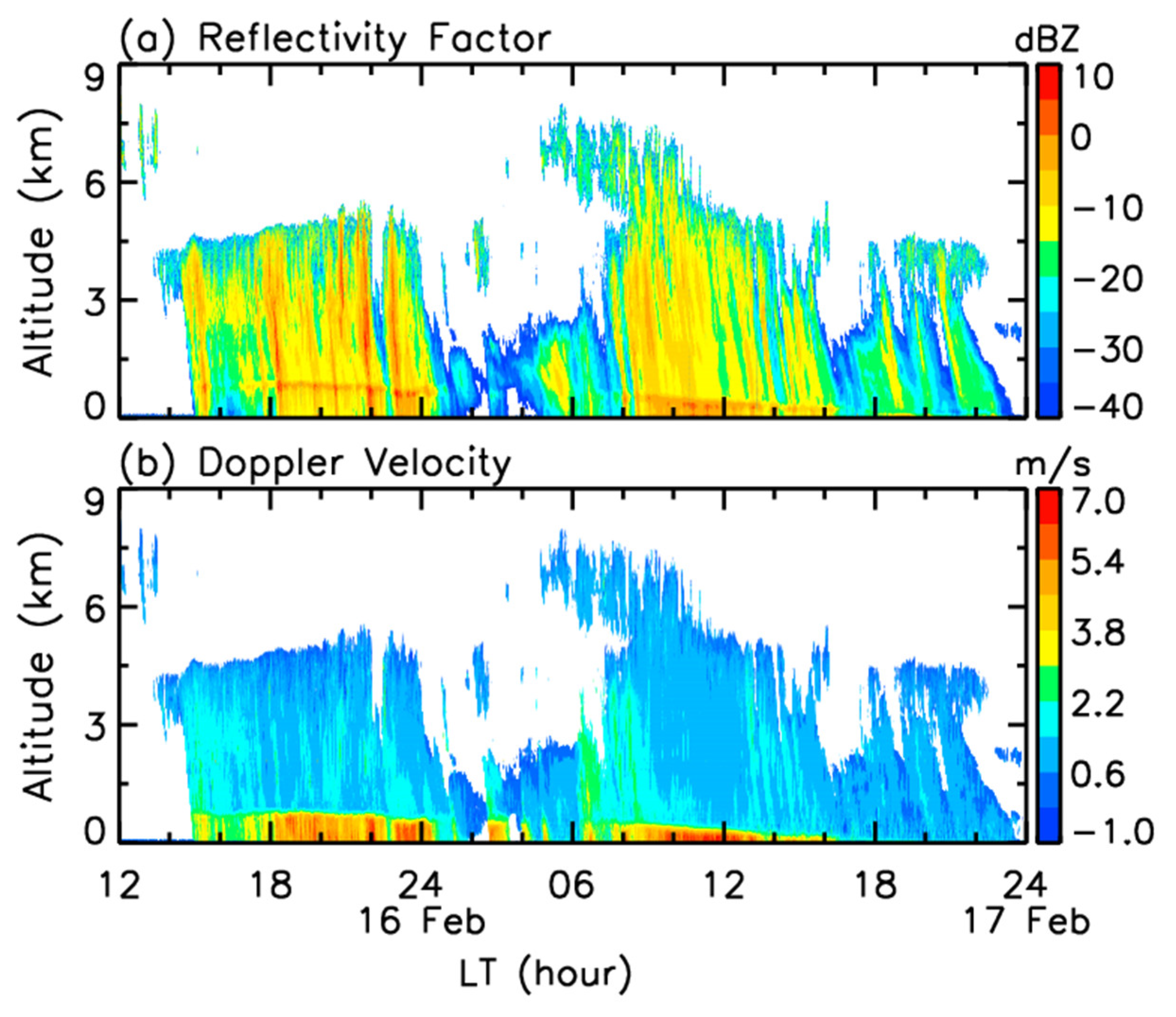
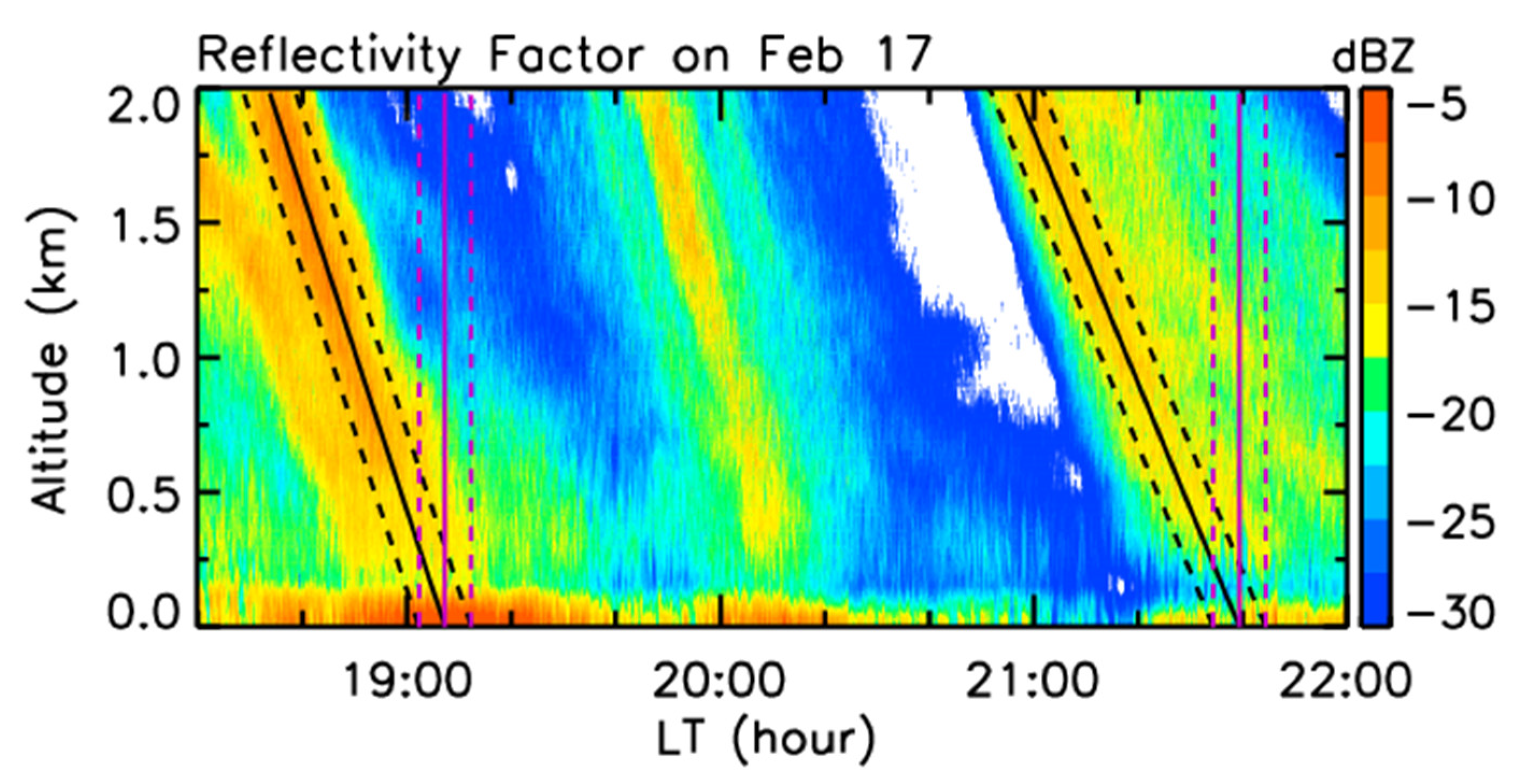
3.1. MMCR Observation during Cooling

Figure 1 shows the reflectivity factor and Doppler velocity (positive downward) from the Ka-band MMCR observation from 12:00 on 16 to 24:00 on 17 February 2022, and Figure 2 presents the evolution of the atmospheric temperature, specific humidity, and specific rainwater and snow-water contents in Wuhan from the ERA5 reanalysis data in the same period. The reanalysis shows that in the period, the temperature on the surface has a maximum value of 7.7 °C at 15:00 on 16 February, and then monotonically decreases to 1.7 °C at 15:00 on 17 February, followed by 0 °C at 19:00 and −0.5 °C at 24:00, without a diurnal cycle. The level of 0 °C falls gradually from the highest altitude of 0.88 km at 17:00 on 16 February to the ground at 19:00 on 17 February. Hence, there is a cooling process in Wuhan during this period with a slightly weaker intensity than a cold surge.

Further, Figure 3 depicts the distribution of temperature and specific humidity at the 1000 hPa level at 15:00 on 16 February from ERA5 reanalysis data. It can clearly be seen that cooling air comes from the northwest, and there is abundant water vapor in the south of Wuhan; in contrast, water vapor decreases rapidly in the north of Wuhan.

One can note from the reflectivity factor in Figure 1 that before 14:00 on 16 February, there are some high-level cirrus clouds above 6 km, and at about 14:00, mid-level clouds occur at a height of 3–4.5 km, whereas soon, rain falls to the ground at 14:58. The cloud top increases slightly to 5.7 km at 22:00, and the clouds dissipate from 24:00 on 16 February to 08:00 on 17 February with intermittent light rain. From 04:48 on 17 February, new high-level clouds from above 6 km and develop downward, leading to intensified rainfalls after 08:00 on 17 February. After 16:00, the ERA5 data indicate a strong reduction in the specific humidity, as shown in Figure 2b, and the cloud height and reflectivity factor have large fluctuations with time. Meanwhile, as the 0 °C level drops to an altitude of only 40 m at 18:00 in the reanalysis, the light rain is evolved into mixed rain and snow, and the precipitation comes to an end at about 23:20 on 17 February.

With the 0 °C level descending during cooling, the melting layer bright band in precipitation shows a clear decline from 0.84 km at 18:20 on 16 February to close to the ground at 16:00 on 17 February. Crossing the bright band, the fall speed of raindrops increases rapidly due to melting raindrop growth via collision and coalescence. In Figure 2, the specific rainwater and snow-water contents in the reanalysis data show spatial and temporal distributions that are consistent with those in the MMCR measurements before 18:00 on 17 February; nevertheless, the reanalysis cannot capture the mixed light rain and snow in the MMCR observations from about 18:00 to 23:20.

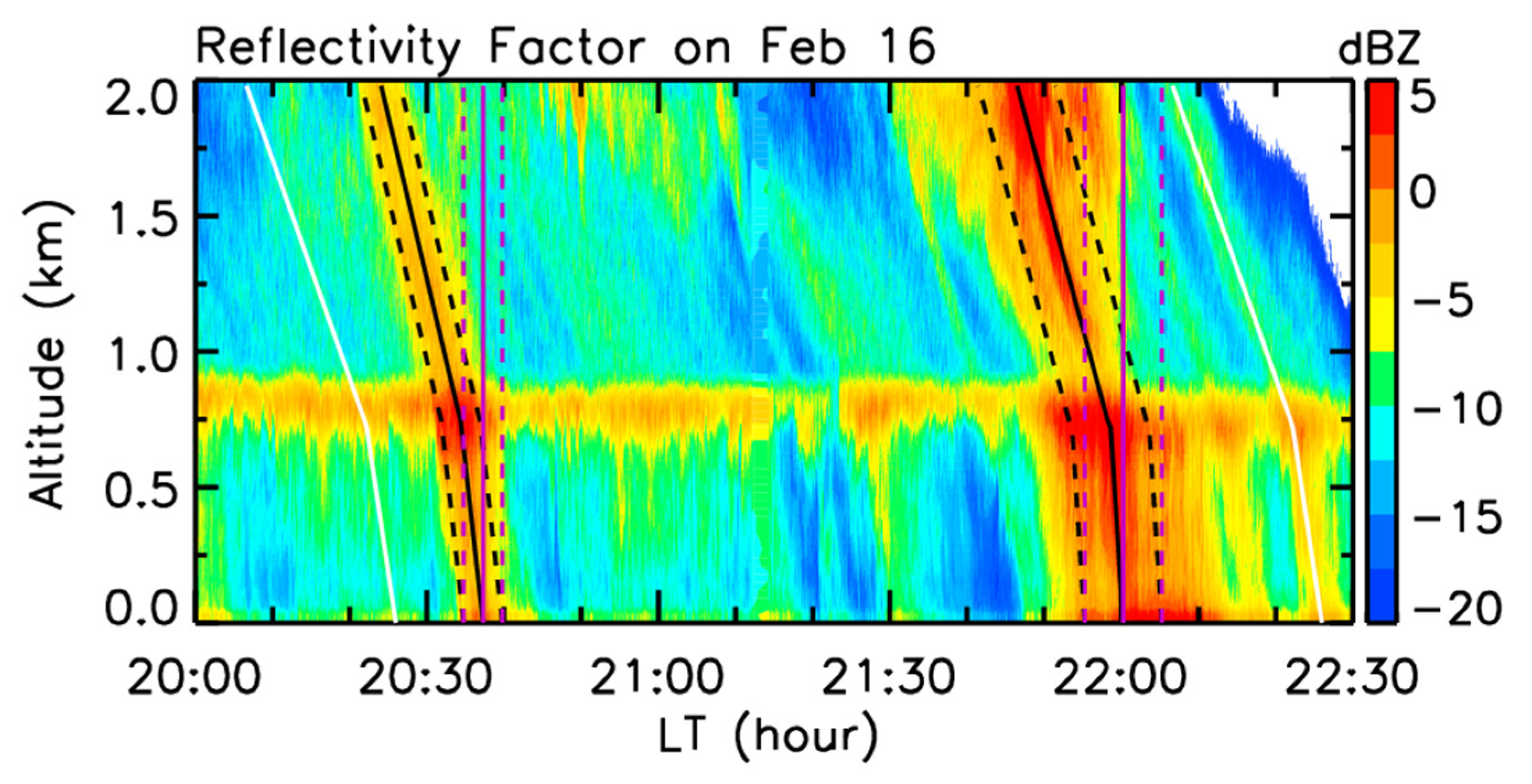
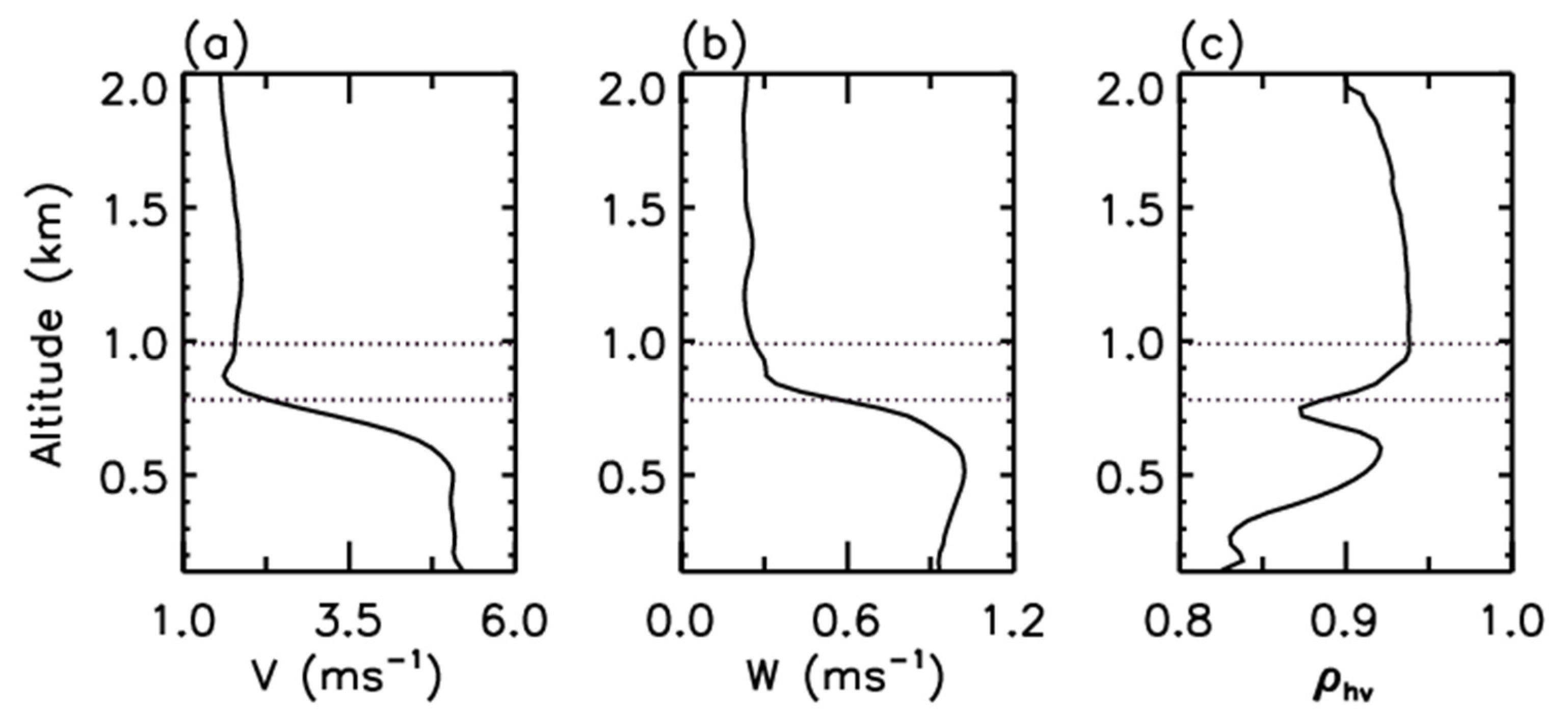
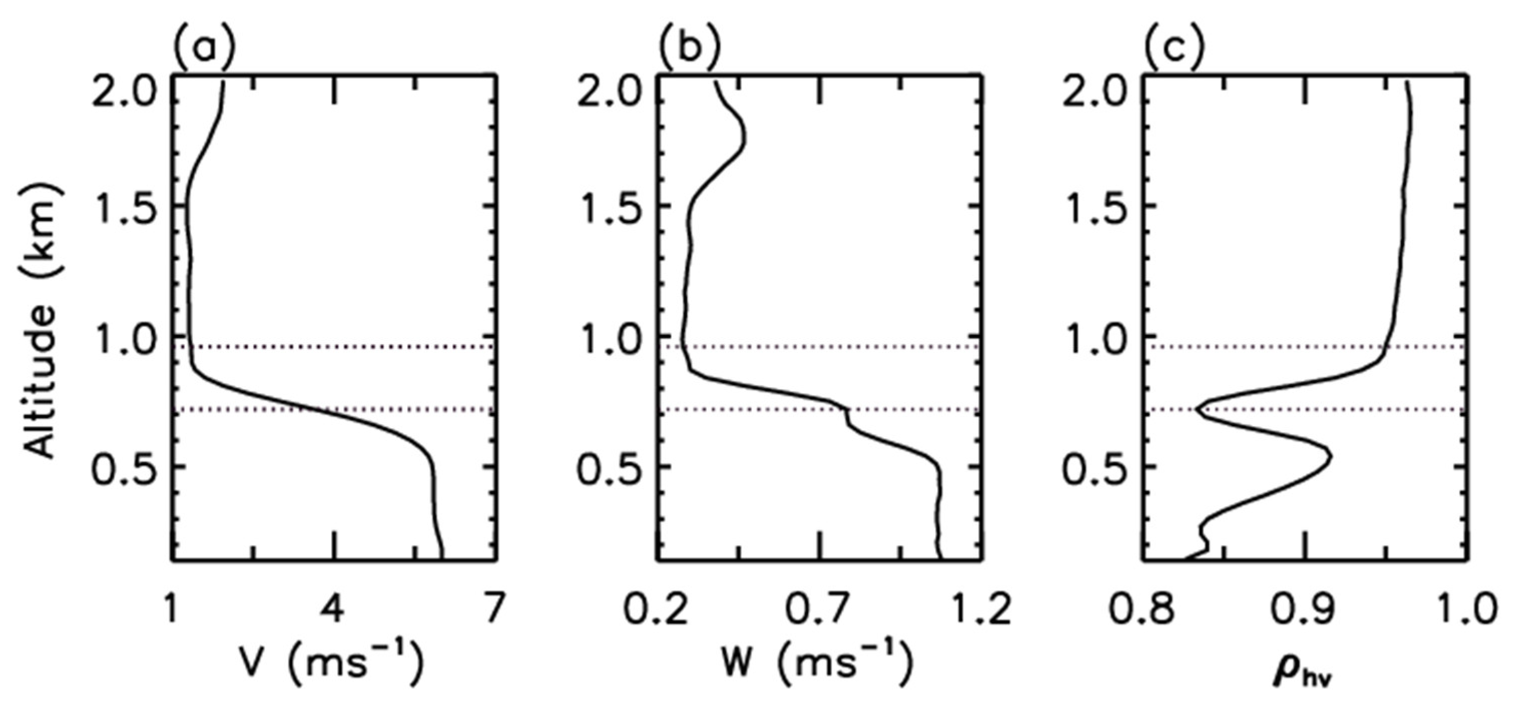
3.2. Bright Band Features in Precipitation

To investigate the variational features of hydrometeors across the melting layer observed by the Ka-band MMCR, we zoom in on the precipitation from 20:00 to 22:30 on 16 February, which is presented in Figure 4. One can note from Figure 4 that there are two periods of relatively strong precipitation with a reflectivity factor larger than −5 dBZ. The first and second periods last for about 5 min and 10 min, respectively. The environmental variation in precipitation particle growth may cause the formation of fall streaks that can be seen in radar measurements. Due to the presence of an atmospheric wind field, the hydrometeors can drift horizontally during their fall; thus, their trails are generally slanted in the height–time section from the radar observations. The slanted trails are referred to as the fall streaks [23], which are clearly shown in Figure 4. For these two periods, we use the solid black line to mark the central times (20:37 and 22:00 on the ground) at which the reflectivity generally has the local maximal values, and then mark the time periods of our attention with the dashed black lines. Although the streak slope can be affected by horizontal wind and its shear, and the microphysical characteristics of hydrometeors (size, density, and phase), the area designated by the dashed black lines is roughly consistent with the one with relatively strong reflectivities, indicating a certain rationality and feasibility of the chosen area. The radar observations in the vertical direction during the two periods are marked by the corresponding purple vertical lines.

For the first period, we calculate the reflectivity factors averaged from 1, 2, and 5 min centered at the intermediate time (20:37 on the ground), which is shown in Figure 5, together with the profile of the temperature from the radiosonde and reanalysis data at 20:00 on 16 February. There are some differences between the radiosonde and reanalysis temperatures. Near the ground, the radiosonde temperature of 6.9 °C is 1.6 °C higher than the reanalysis temperature of 5.3 °C, and the 0 °C level is at the height of 0.9 km in the radiosonde observation but 0.8 km in the reanalysis data, indicating the influence of rapid cooling on the accuracy of reanalysis temperature. Along the fall streaks, the reflectivity in the bright band has the peak values of 1 min average 2.76 dBZ at 0.75 km, 2 min average 2.54 dBZ at 0.75 km, and 5 min average 1.60 dBZ at 0.78 km, showing a slight dip in the bright band with the slight enhancement of light rain. The results are consistent with previous reports that the bright band is about 0.1 km lower than the 0 °C level and displays an obvious dip as rainfall intensifies significantly [22,46]. Previous observations and modeling studies reported that the maximum reflectivity of the bright band (bright band peak) may be located at 0–0.9 km below the freezing level, which depends on latitude, season, geography, radar operating wavelength, and the type and size of frozen hydrometeor particles [25,47,48,49,50,51]. It can be noted in Figure 5 that there is a minimum reflectivity (dark valley) above the bright band. In previous weather radar and millimeter wave radar observations, the dark valley was proposed to be caused by the combination of ice particle aggregation and non-Rayleigh scatter effects [22,35,52,53]. In the 5 min average reflectivity, the dark valley at 0.99 km is 0.21 km higher but 6.03 dB weaker than the bright band peak. In addition, compared with those along the fall streaks, the reflectivities along the vertical direction show a weaker peak in the bright band, but a larger increase in the melting layer, which can lead to the misconceptions of faster melting of ice particles and more frequent collision–coalescence of raindrops in the melting layer. Hence, in the presence of atmospheric wind, it is significant to infer the microphysical processes in precipitation from the radar observations along the fall streaks instead of the vertical direction.

Figure 6 depicts the Doppler velocity, Doppler spectrum width, and cross-correlation coefficient averaged along the fall streaks from the MMCR observation for 5 min. It can be seen from Figure 6 that with the phase transition of hydrometeors, the reflectivity is strengthened mainly due to the increase in the dielectric constant from the melting of ice to water in the melting layer, and then decreases with the reduction in raindrop concentrations caused by the increasing fall speeds of raindrops; in this case, the bright band is observed in the reflectivity factor. In the melting layers, due to the droplet spectrum being broadened by the collision, coalescence, and even breakup of hydrometeors and the effects of turbulence and wind shear, the Doppler spectrum width also increases rapidly. As ice particles and snowflakes melt into raindrops, the Doppler velocity (spectrum width) of hydrometeors increases rapidly from the minimal value of 1.61 (0.31) ms⁻¹ at 0.87 km to 4.89 (1.02) ms⁻¹ at 0.57 km, and the height of 0.87 km is slightly lower than the 0.99 km of the dark valley, whereas the correlation coefficient displays a quick drop from 0.94 at the dark valley to 0.88 at the bright band peak, followed by a process of rapid growth and recovery. In the observation of S-band weather radar, the mean vertical profile of the correlation coefficient constructed through a series of range-height indicator (RHI) scans showed that the correlation coefficient decreases from about 0.91 to 0.84 after crossing the melting layer [54], and the correlation could drop to 0.85 for different elevation angles [55]. Early studies suggested that the correlation coefficient is influenced by mixed-phase hydrometeors, radar operating frequency, antenna elevation angles, and beam broadening [46,55,56,57].

Similarly, for the second period centered at 22:00 on the ground, Figure 7 presents the 1, 5, and 10 min average reflectivities along the fall streaks and in the vertical direction, respectively, together with the temperature at 22:00 from the reanalysis for reference. Figure 8 illustrates the evolution of the Doppler velocity, spectrum width, and cross-correlation coefficient averaged from 10 min along the fall streaks. The 0° level is located at 0.77 km from the ERA5 data. The bright band peak derived from 1 (5 and 10) min average reflectivity is located at 0.69 (0.72 and 0.72) km with the value of 6.43 (5.58 and 4.36) dBZ, which is stronger than that in the first period; thus, the concentrations and/or sizes of precipitation particles are slightly larger relative to those in the first period. Based on the 5 and 10 min average reflectivities, the dark valley is at 0.21 and 0.24 km above the bright band peak, but its magnitude is about 9.0 and 8.72 dB smaller relative to the bright band peak, respectively, whereas the reflectivity is enhanced by about 12.5 dB from the dark valley to the bright band peak based on the observation in the vertical direction, indicating quicker melting of hydrometeors, or a longer melting duration of larger snowflakes if the melting is discussed from the vertical observation.

In Figure 8, the variations in the Doppler velocity, spectrum width, and correlation coefficient around the melting layer are in good agreement with those in Figure 6. Nevertheless, owing to the larger reflectivity increment from the dark valley to the bright band peak, these parameters show more significant changes compared with those in the first period. Across the bright band, the fall velocity and Doppler spectrum width increase by about 4.45 ms⁻¹ and 0.76 ms⁻¹, being more than those of 3.28 ms⁻¹ and 0.71 ms⁻¹ in Figure 6, respectively. The cross-correlation coefficient decreases to 0.83 at the bright band peak from 0.95 at the dark valley, and the reduced intensity of 0.12 is larger than that of 0.06 in Figure 6.

For general consideration, we calculate the mean profiles of radar observations every 5 min from 20:26 to 22:26, shown with the two white lines in Figure 4. By determining the bright band peak in each profile, we derived the average values in a bright band peak coordinate (i.e., setting its height to be 0) from these profiles, and the results are presented in Figure 9 and Figure 10. Figure 9 illustrates that the mean dark valley is 0.24 km higher relative to the bright band peak, with a magnitude of −9.95 dBZ, which is less than the −1.92 dBZ magnitude of the bright band peak. In Figure 10, the fall velocity (spectrum width) of rainfall particles shows a growth of about 3.52 (0.75) ms⁻¹ after crossing the bright band. The correlation coefficient declines from 0.93 at the dark valley to 0.87 at the bright band peak. These variational characteristics are similar to those in the two periods above; thus, this analysis quantitatively exhibits the evolution of the Doppler velocity, spectrum width, and correlation coefficient around the melting layer in precipitation during cooling, and the features are more obvious with the enhancement of precipitation.

3.3. Observation of Mixed Rain and Snow

As the surface temperature approaches the 0 °C level, the weak rain evolves into mixed rain and snow after about 18:00 on 17 quantitatively. Here, we examine the Ka-band MMCR observation of mixed rain and snow, and Figure 11 zooms in on the reflectivity from 18:20 to 21:50 on 17 February. We analyze the relatively strong precipitation with a reflectivity factor larger than −20 dBZ in the chosen two durations (as the third and fourth periods). Both the two durations are 10 min, and their central times are 19:07 and 21:39 on the ground, respectively. In Figure 11, the reflectivities along the fall streaks and the vertical direction are marked with black and purple lines, respectively.

Figure 12 shows the 10 min average reflectivities along the fall streaks and the vertical direction from the Ka-band MMCR observation in the two periods, as well as the profile of the temperature from the radiosonde and reanalysis data at 20:00 on 17 February. In the third period, as the height reduces, the reflectivity factor tends to decrease slowly along the fall streaks, but to increase gradually in the vertical direction, whereas the reflectivity drops quickly from about 0.5 km in the fourth period. There is not a bright band in the reflectivity profile due to the surface temperature being close to 0 °C.

Figure 13 and Figure 14 present the Doppler velocity, Doppler spectrum width, and cross-correlation coefficient averaged along the fall streaks in the third and fourth periods. Relative to those in the first and second periods, the reflectivities are weaker in the third and fourth periods; thus, the hydrometeors have smaller sizes and fall velocities. It can be noted that from about 0.7 (0.6) km down to 0.5 (0.4) km in the third (fourth) period, the Doppler spectrum width shows an obvious enlargement, but the correlation coefficient evidently decreases by about 0.07 (0.06). The correlation reduction can be caused by the enhanced irregularities and broadened size distributions of ices and snowflakes, and the fact that ices and snowflakes are wetted and become spongy [58,59,60]. The correlation coefficient may be less than 0.8 and even 0.6 in the wet snow for S-, C- and X-band radars [27,56,60,61,62].

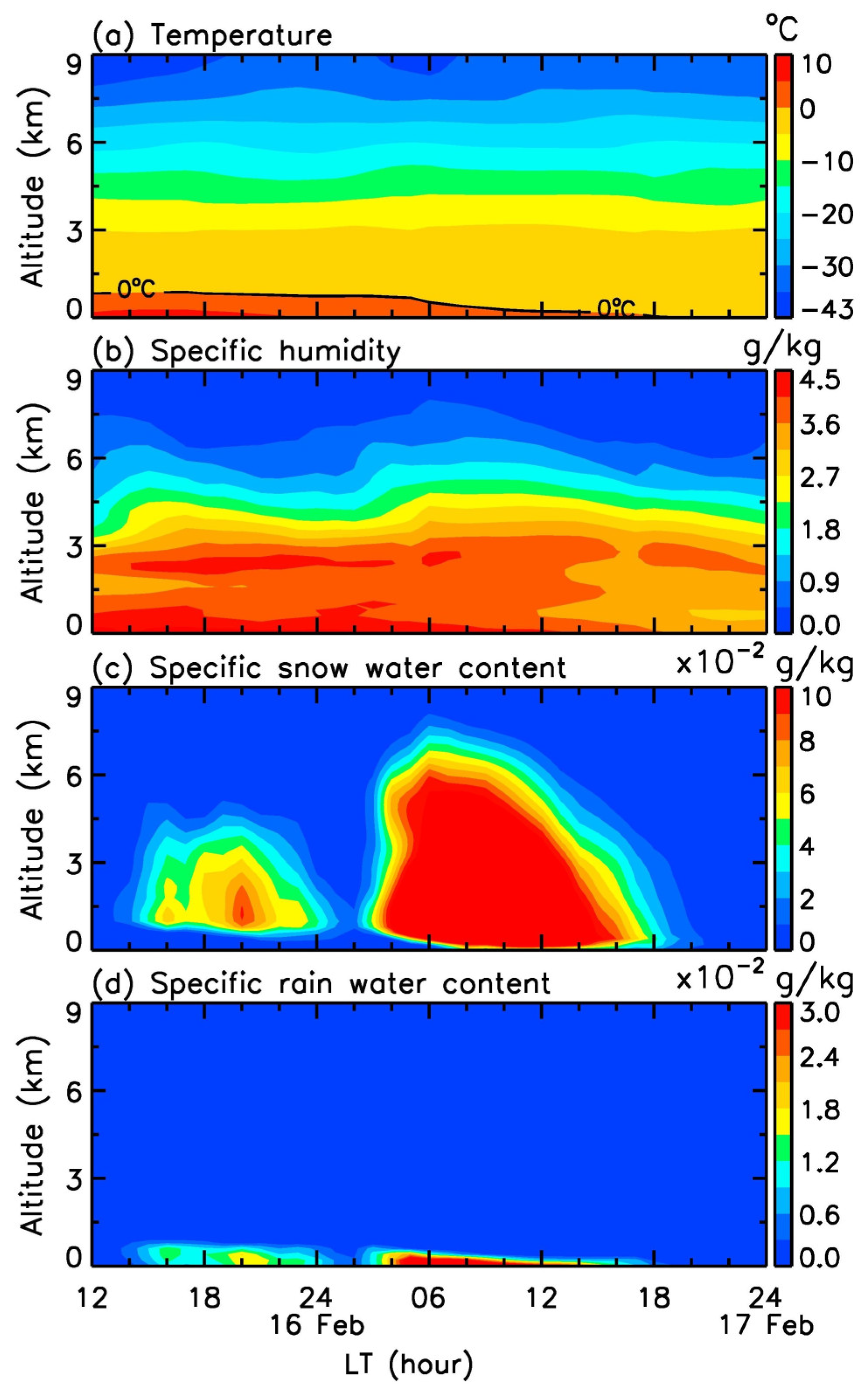
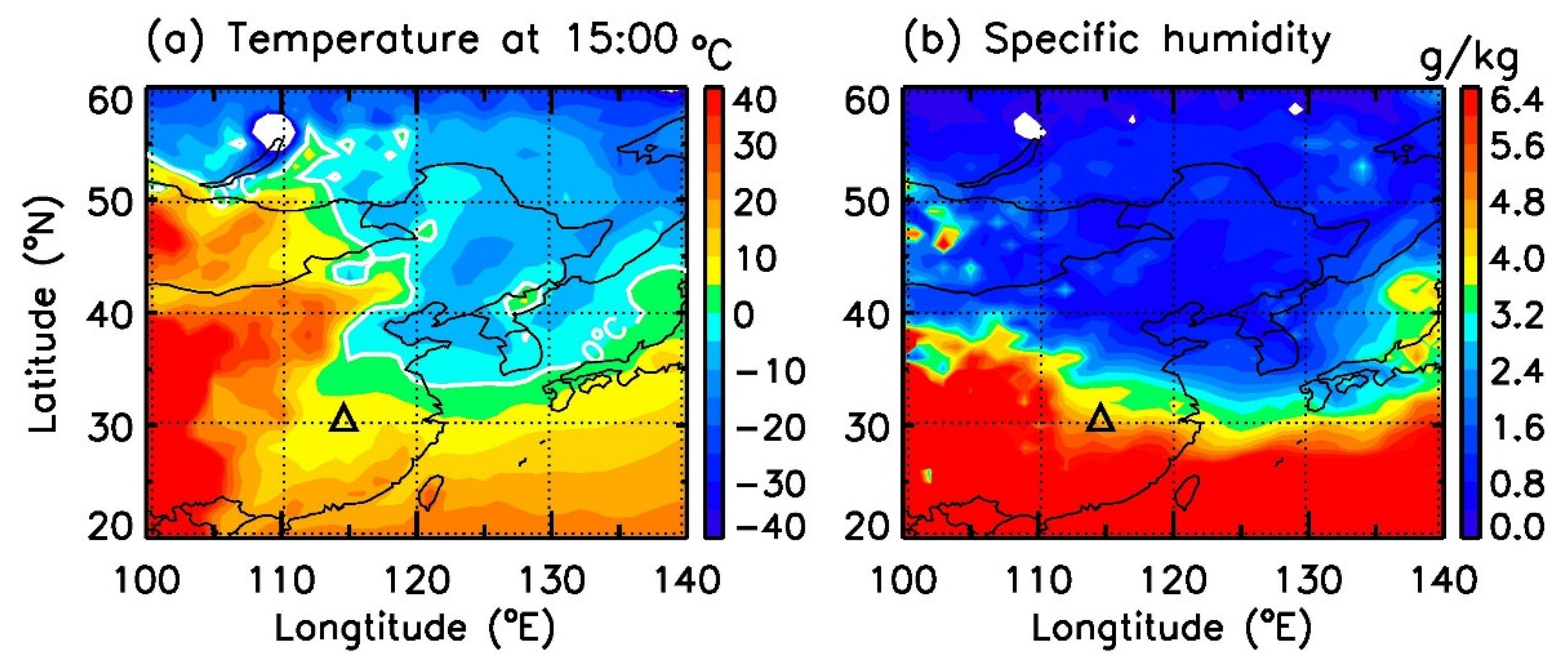
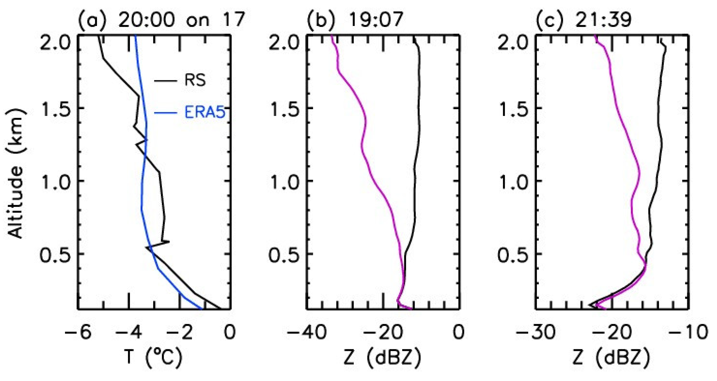
4. Atmospheric Conditions

Here, we investigate the atmospheric conditions during cooling and weak precipitation based on the radiosonde and reanalysis data. Figure 15 presents the temperature, zonal wind (positive eastward), meridional wind (positive northward), specific humidity, and relative humidity from the ground to 9 km at 20:00 on 16 February and at 8:00 on 17 and 18 February, and Figure 16 depicts the zonal, meridional, and vertical (in units of Pa s⁻¹, positive downward) winds between 12:00 on 16 February and 24:00 on 17 February from the reanalysis data. In Figure 15, the temperature, horizontal winds, and specific humidity between the two data are approximately consistent with each other, whereas their profiles are smoother in the reanalysis than in the radiosonde observation.

Figure 15 and Figure 16 illustrate that in the zonal direction, the easterly is changed to the westerly at about 2 km, while in the meridional direction, the northerly is reversed to be the southerly at about 1 km. The frigid north wind from the ground to 1 km causes cooling, and the surface temperature drops from about 7.3 °C at 20:00 on 16 February to 2.8 °C at 08:00 on 17 February, and to −0.5 °C at 08:00 on 18 February. It can be noted from the radiosonde observation at 20:00 on 16 February that the temperature lapse rate is 8.65 °C km⁻¹ below 1 km, and decreases to 3.62 °C km⁻¹ at about 1–2 km with the reversal from the northerly to the southerly. Furthermore, as the zonal wind is reversed at about 2 km, a thermal inversion layer occurs around 2 km, and the temperature lapse rate is changed to be 5.67 °C km⁻¹ above 3 km. Accordingly, Figure 15d shows that the warm southeasterly at about 1–2 km and southwesterly above 2 km is abundant in water vapor. Owing to the uplift of the warm moist air by the cold air from the north, the relative humidity reaches saturation at about 1 km. As shown in Figure 15e, the saturated water vapor nearly covers the height range of 1–5 km, which is in good agreement with the MMCR measurement in Figure 1 that the cloud top is located at about 5 km, and the precipitation occurs below about 5 km at 20:00 on 16 February. The reanalysis data in Figure 16 indicate that there is a downdraft at 3–6 km around 24:00 on 16 February, which is possibly responsible for the cloud dissipation and rain abatement in the MMCR observation.

At 08:00 on 17 February, Figure 15 shows that the thermal inversion layer disappears, causing the small vertical changes in temperature and specific humidity below 3 km, and the water vapor reaches saturation from the ground up to 5 km in favor of the continuation of precipitation. It can be seen from the reanalysis in Figure 16c that a strong downdraft arises after 18:00 on 17 February, implying strong cloud dissipation; thus, the reanalysis specific rain water and specific snow water contents approach zero from the ground to the high levels, as shown in Figure 2. However, in Figure 1, the MMCR observes clouds and light precipitation with clear fall streaks. This discrepancy illustrates the difficulty of the reanalysis to accurately capture the vertical winds, relative to the relatively stable horizontal wind field.

At 8:00 on 18 February, the temperature near the ground is below 0 °C, and the specific humidity decreases obviously; meanwhile, the relative humidity is less than 90%, meaning that the precipitation has stopped.

Finally, to assess the stability of the atmosphere during cooling, we derive the buoyant frequency squared (N²) and Richardson number (Ri) from the ERA5 reanalysis data, which are depicted in Figure 17. Owing to the large lapse rate by the cold air from the north, there is a thin layer over the ground with a low buoyancy frequency (N² < 1 × 10⁻⁴ s⁻²). As we expected, the atmosphere shows fine stability in cooling and precipitation because of the large-scale uplift caused by the encounter of cold and warm air masses. From the near surface to high altitudes, the Richardson number is larger than one except for a quite shallow layer close to the ground. Hence, there are no conditions for convective bubble generation, which is different from convective precipitation with the occurrence of intense atmospheric instability.

5. Summary

In this paper, we study the stratiform precipitation during cooling on 16–17 February 2022 based on a Ka-band MMCR’s observation in Wuhan combined with ERA5 reanalysis and radiosonde data, and discuss the characteristics of the melting layer and the atmospheric conditions in the stratiform precipitation.

The reanalysis and radiosonde data show that the temperature on the surface drops by about 8 °C, with the lowest value less than 0 °C, in the two days because of the strong cold air from the north, meaning that the cooling is close to a cold surge, and the 0 °C level falls gradually from the highest altitude of 0.88 km to the ground at 19:00 on 17 February. Above the cold northeasterly wind, there is the warm and humid air from the southeast and southwest, which is lifted by the cold air; thus, the cooling is beneficial to stratiform cloud formation and sustained light precipitation. The radar observation indicates that mid-level clouds arise at 3–4.5 km at about 14:00 on 16 February, and an hour later, light rain falls to the ground. Subsequently, the clouds gradually develop upward and the weak precipitation continues with reflectivities of about −15–5 dBZ. From 24:00 on 16 February to 08:00 on 17 February, the mid- and high-level clouds dissipate with intermittent precipitation possibly due to the downdraft over 3 km shown in the reanalysis. After this, with the occurrence and downward evolution of new high-level clouds, the precipitation continues until about 23:20 on 17 February. Nevertheless, the light rain is changed to sleet and light snow from about 18:00 as the temperature on the ground gradually drops below 0 °C. Before 18:00 on 17 February, the spatial and temporal distributions of specific rainwater and snow-water contents in the reanalysis data are in good agreement with those in the MMCR observations, whereas the reanalysis cannot capture the mixed light rain and snow after 18:00 since there is a strong downdraft from near the ground to about 4 km in the reanalysis.

As the 0 °C level descends, the bright band drops gradually. The peak of the bright band is about 0.1 km lower than the 0 °C level in the weak precipitation and shows a slight dip with the intensification of precipitation, and there is a dark valley with the minimal reflectivity located about 0.21–0.24 km above the bright band peak. Across the bright band, the Doppler velocity and spectrum width of rainfall particles increases significantly. For the chosen 5 and 10 min averages in the two periods, the reflectivity is enhanced by about 6.03 and 8.72 dB from the dark valley to the bright band peak, respectively. Accordingly, across the bright band, the Doppler velocity (spectrum width) of hydrometeors increases by 3.28 (0.71) ms⁻¹ and 4.45 (0.76) ms⁻¹, while the cross-correlation coefficient decreases from 0.94 (0.95) to 0.88 (0.83), respectively. As the surface temperature approaches the 0 °C level, the light rain evolves into mixed rain and snow, and the bright band disappears in the profile of reflectivity. Nevertheless, due to the enlargement of the Doppler spectrum width of falling hydrometeors, the cross-correlation coefficient evidently decreases by about 0.07 (0.06). In the stratiform precipitation during cooling, the atmospheric stability is fine due to the lifting of warm air. In addition, the analysis indicates that it is significant to investigate the melting process along the fall streaks in the presence of strong wind shear because the melting may be overestimated from the vertical perspective.

Finally, it is important to note that the reanalysis data alone cannot capture the transition to the mixed rain and snow regime on the ground; however, at this time, dangerous freezing rain or sleet could occur on the surface. In this way, only relying on reanalysis data (and potentially also on outputs from atmospheric models that only assimilate reanalysis data without high-resolution cloud radar measurements directly) will not be sufficient to investigate the full scope of hazards posed by cold surges or the conditions under which they occur. Therefore, a detailed analysis of cold surges and their impact on society will probably need to include an investigation of high-resolution and high-sensitivity radar data that can capture the full spectrum of relevant microphysical processes in clouds and precipitation.

References

1. Quante, M. The Role of Clouds in the Climate System. J. Phys. IV Proc. 2004, 121, 61–86. [Google Scholar] [CrossRef]
2. Stephens, G.L. Cloud Feedbacks in the Climate System: A Critical Review. J. Clim. 2005, 18, 237–273. [Google Scholar] [CrossRef]
3. Szeto, K.K.; Lin, C.A.; Stewart, R.E. Mesoscale Circulations Forced by Melting Snow. Part I: Basic Simulations and Dynamics. J. Atmos. Sci. 1988, 45, 1629–1641. [Google Scholar] [CrossRef]
4. Han, X.; Xue, H.; Zhao, C.; Lu, D. The Roles of Convective and Stratiform Precipitation in the Observed Precipitation Trends in Northwest China during 1961–2000. Atmos. Res. 2016, 169, 139–146. [Google Scholar] [CrossRef]
5. Houze, R.A., Jr.; Rasmussen, K.L.; Zuluaga, M.D.; Brodzik, S.R. The Variable Nature of Convection in the Tropics and Subtropics: A Legacy of 16 Years of the Tropical Rainfall Measuring Mission Satellite. Rev. Geophys. 2015, 53, 994–1021. [Google Scholar] [CrossRef] [PubMed]
6. Wu, Z.; Huang, Y.; Zhang, Y.; Zhang, L.; Lei, H.; Zheng, H. Precipitation Characteristics of Typhoon Lekima (2019) at Landfall Revealed by Joint Observations from GPM Satellite and S-Band Radar. Atmos. Res. 2021, 260, 105714. [Google Scholar] [CrossRef]
7. Wang, R.; Tian, W.; Chen, F.; Wei, D.; Luo, J.; Tian, H.; Zhang, J. Analysis of Convective and Stratiform Precipitation Characteristics in the Summers of 2014–2019 over Northwest China Based on GPM Observations. Atmos. Res. 2021, 262, 105762. [Google Scholar] [CrossRef]
8. Wen, L.; Chen, G.; Yang, C.; Zhang, H.; Fu, Z. Seasonal Variations in Precipitation Microphysics over East China Based on GPM DPR Observations. Atmos. Res. 2023, 293, 106933. [Google Scholar] [CrossRef]
9. Gettelman, A.; Liu, X.; Barahona, D.; Lohmann, U.; Chen, C. Climate Impacts of Ice Nucleation. J. Geophys. Res. Atmos. 2012, 117, D20201. [Google Scholar] [CrossRef]
10. He, J.; Zheng, J.; Zeng, Z.; Che, Y.; Zheng, M.; Li, J. A Comparative Study on the Vertical Structures and Microphysical Properties of Stratiform Precipitation over South China and the Tibetan Plateau. Remote Sens. 2021, 13, 2897. [Google Scholar] [CrossRef]
11. Houze, R.A. Stratiform Precipitation in Regions of Convection: A Meteorological Paradox? Bull. Am. Meteorol. Soc. 1997, 78, 2179–2196. [Google Scholar] [CrossRef]
12. Ruiz-Leo, A.M.; Hernández, E.; Queralt, S.; Maqueda, G. Convective and Stratiform Precipitation Trends in the Spanish Mediterranean Coast. Atmos. Res. 2013, 119, 46–55. [Google Scholar] [CrossRef]
13. Schumacher, C.; Houze, R.A. Stratiform Rain in the Tropics as Seen by the TRMM Precipitation Radar. J. Clim. 2003, 16, 1739–1756. [Google Scholar] [CrossRef]
14. Hou, T.; Lei, H.; Hu, Z. A Comparative Study of the Microstructure and Precipitation Mechanisms for Two Stratiform Clouds in China. Atmos. Res. 2010, 96, 447–460. [Google Scholar] [CrossRef]
15. Garcia-Benadí, A.; Bech, J.; Gonzalez, S.; Udina, M.; Codina, B. A New Methodology to Characterise the Radar Bright Band Using Doppler Spectral Moments from Vertically Pointing Radar Observations. Remote Sens. 2021, 13, 4323. [Google Scholar] [CrossRef]
16. Ghada, W.; Casellas, E.; Herbinger, J.; Garcia-Benadí, A.; Bothmann, L.; Estrella, N.; Bech, J.; Menzel, A. Stratiform and Convective Rain Classification Using Machine Learning Models and Micro Rain Radar. Remote Sens. 2022, 14, 4563. [Google Scholar] [CrossRef]
17. Matrosov, S.Y. Distinguishing between Warm and Stratiform Rain Using Polarimetric Radar Measurements. Remote Sens. 2021, 13, 214. [Google Scholar] [CrossRef]
18. Gray, W.R.; Cluckie, I.D.; Griffith, R.J. Aspects of Melting and the Radar Bright Band. Meteorol. Appl. 2001, 8, 371–379. [Google Scholar] [CrossRef]
19. White, A.B.; Gottas, D.J.; Strem, E.T.; Ralph, F.M.; Neiman, P.J. An Automated Brightband Height Detection Algorithm for Use with Doppler Radar Spectral Moments. J. Atmos. Ocean Technol. 2002, 19, 687–697. [Google Scholar] [CrossRef]
20. Evans, S. Dielectric Properties of Ice and Snow—A Review. J. Glaciol. 1965, 5, 773–792. [Google Scholar] [CrossRef]
21. Meneghini, R.; Liao, L. Effective Dielectric Constants of Mixed-Phase Hydrometeors. J. Atmos. Ocean Technol. 2000, 17, 628–640. [Google Scholar] [CrossRef]
22. Fabry, F.; Zawadzki, I. Long-Term Radar Observations of the Melting Layer of Precipitation and Their Interpretation. J. Atmos. Sci. 1995, 52, 838–851. [Google Scholar] [CrossRef]
23. Li, H.; Moisseev, D. Two Layers of Melting Ice Particles Within a Single Radar Bright Band: Interpretation and Implications. Geophys. Res. Lett. 2020, 47, e2020GL087499. [Google Scholar] [CrossRef]
24. Yi, Y.; Yi, F.; Liu, F.; Zhang, Y.; Yu, C.; He, Y. Microphysical Process of Precipitating Hydrometeors from Warm-Front Mid-Level Stratiform Clouds Revealed by Ground-Based Lidar Observations. Atmos. Chem. Phys. 2021, 21, 17649–17664. [Google Scholar] [CrossRef]
25. Di Girolamo, P.; Summa, D.; Cacciani, M.; Norton, E.G.; Peters, G.; Dufournet, Y. Lidar and Radar Measurements of the Melting Layer: Observations of Dark and Bright Band Phenomena. Atmos. Chem. Phys. 2012, 12, 4143–4157. [Google Scholar] [CrossRef]
26. Wei, T.; Xia, H.; Wu, K.; Yang, Y.; Liu, Q.; Ding, W. Dark/Bright Band of a Melting Layer Detected by Coherent Doppler Lidar and Micro Rain Radar. Opt. Express 2022, 30, 3654. [Google Scholar] [CrossRef]
27. Kumjian, M.R.; Mishra, S.; Giangrande, S.E.; Toto, T.; Ryzhkov, A.V.; Bansemer, A. Polarimetric Radar and Aircraft Observations of Saggy Bright Bands during MC3E. J. Geophys. Res. Atmos. 2016, 121, 3584–3607. [Google Scholar] [CrossRef]
28. Dias Neto, J.; Kneifel, S.; Ori, D.; Trömel, S.; Handwerker, J.; Bohn, B.; Hermes, N.; Mühlbauer, K.; Lenefer, M.; Simmer, C. The TRIple-Frequency and Polarimetric Radar Experiment for Improving Process Observations of Winter Precipitation. Earth Syst. Sci. Data 2019, 11, 845–863. [Google Scholar] [CrossRef]
29. Arulraj, M.; Barros, A.P. Improving Quantitative Precipitation Estimates in Mountainous Regions by Modelling Low-Level Seeder-Feeder Interactions Constrained by Global Precipitation Measurement Dual-Frequency Precipitation Radar Measurements. Remote Sens. Environ. 2019, 231, 111213. [Google Scholar] [CrossRef]
30. Kühnlein, M.; Appelhans, T.; Thies, B.; Nauss, T. Improving the Accuracy of Rainfall Rates from Optical Satellite Sensors with Machine Learning—A Random Forests-Based Approach Applied to MSG SEVIRI. Remote Sens. Environ. 2014, 141, 129–143. [Google Scholar] [CrossRef]
31. Zawadzki, I.; Szyrmer, W.; Bell, C.; Fabry, F. Modeling of the Melting Layer. Part III: The Density Effect. J. Atmos. Sci. 2005, 62, 3705–3723. [Google Scholar] [CrossRef]
32. Leinonen, J.; von Lerber, A. Snowflake Melting Simulation Using Smoothed Particle Hydrodynamics. J. Geophys. Res. Atmos. 2018, 123, 1811–1825. [Google Scholar] [CrossRef]
33. Billault-Roux, A.-C.; Grazioli, J.; Delanoë, J.; Jorquera, S.; Pauwels, N.; Viltard, N.; Martini, A.; Mariage, V.; Gac, C.L.; Caudoux, C.; et al. ICE GENESIS: Synergetic Aircraft and Ground-Based Remote Sensing and In Situ Measurements of Snowfall Microphysical Properties. Bull. Am. Meteorol. Soc. 2023, 104, E367–E388. [Google Scholar] [CrossRef]
34. Smyth, T.J.; Illingworth, A.J. Radar Estimates of Rainfall Rates at the Ground in Bright Band and Non-Bright Band Events. Q. J. R. Meteorol. Soc. 1998, 124, 2417–2434. [Google Scholar] [CrossRef]
35. Sassen, K.; Campbell, J.R.; Zhu, J.; Kollias, P.; Shupe, M.; Williams, C. Lidar and Triple-Wavelength Doppler Radar Measurements of the Melting Layer: A Revised Model for Dark- and Brightband Phenomena. J. Appl. Meteorol. 2005, 44, 301–312. [Google Scholar] [CrossRef]
36. Devisetty, H.K.; Jha, A.K.; Das, S.K.; Deshpande, S.M.; Krishna, U.V.M.; Kalekar, P.M.; Pandithurai, G. A Case Study on Bright Band Transition from Very Light to Heavy Rain Using Simultaneous Observations of Collocated X- and Ka-Band Radars. J. Earth Syst. Sci. 2019, 128, 136. [Google Scholar] [CrossRef]
37. Jha, A.; Kalapureddy, M.; Devisetty, H.; Deshpande, S.; Pandithurai, G. A Case Study on Large-Scale Dynamical Influence on Bright Band Using Cloud Radar during the Indian Summer Monsoon. Meteorol. Atmos. Phys. 2019, 131, 505–515. [Google Scholar] [CrossRef]
38. Frich, P.; Alexander, L.; Della-Marta, P.; Gleason, B.; Haylock, M.; Klein Tank, A.; Peterson, T. Observed Coherent Changes in Climatic Extremes during the Second Half of the Twentieth Century. Clim. Res. 2002, 19, 193–212. [Google Scholar] [CrossRef]
39. Roland, J.; Matter, S.F. Variability in Winter Climate and Winter Extremes Reduces Population Growth of an Alpine Butterfly. Ecology 2013, 94, 190–199. [Google Scholar] [CrossRef] [PubMed]
40. Johnson, N.C.; Xie, S.-P.; Kosaka, Y.; Li, X. Increasing Occurrence of Cold and Warm Extremes during the Recent Global Warming Slowdown. Nat. Commun. 2018, 9, 1724. [Google Scholar] [CrossRef] [PubMed]
41. Probert-Jones, J.R. The Radar Equation in Meteorology. Q. J. R. Meteorol. Soc. 1962, 88, 485–495. [Google Scholar] [CrossRef]
42. Doviak, R.; Zrnic, S. Doppler Radar and Weather Observations, 2nd ed.; Dover Press: Mineola, NY, USA, 2006; ISBN 0486450600. [Google Scholar]
43. Ryzhkov, A.; Zrnic, D. Radar Polarimetry for Weather Observations; Springer Nature Switzerland AG: Cham, Switzerland, 2019; ISBN 978-3-030-05092-4. [Google Scholar]
44. Fang, J.; Huang, K.; Du, M.; Zhang, Z.; Cao, R.; Yi, F. Investigation on Cloud Vertical Structures Based on Ka-Band Cloud Radar Observations at Wuhan in Central China. Atmos. Res. 2023, 281, 106492. [Google Scholar] [CrossRef]
45. Hersbach, H.; Bell, B.; Berrisford, P.; Hirahara, S.; Horányi, A.; Muñoz-Sabater, J.; Nicolas, J.; Peubey, C.; Radu, R.; Schepers, D.; et al. The ERA5 Global Reanalysis. Q. J. R. Meteorol. Soc. 2020, 146, 1999–2049. [Google Scholar] [CrossRef]
46. Brandes, E.A.; Ikeda, K. Freezing-Level Estimation with Polarimetric Radar. J. Appl. Meteorol. Climatol. 2004, 43, 1541–1553. [Google Scholar] [CrossRef]
47. Harris, G.N.; Bowman, K.P.; Shin, D.-B. Comparison of Freezing-Level Altitudes from the NCEP Reanalysis with TRMM Precipitation Radar Brightband Data. J. Clim. 2000, 13, 4137–4148. [Google Scholar] [CrossRef]
48. Leary, C.A.; Houze, R.A. Melting and Evaporation of Hydrometeors in Precipitation from the Anvil Clouds of Deep Tropical Convection. J. Atmos. Sci. 1979, 36, 669–679. [Google Scholar] [CrossRef]
49. Thurai, M.; Deguchi, E.; Iguchi, T.; Okamoto, K. Freezing Height Distribution in the Tropics. Int. J. Satell. Commun. Netw. 2003, 21, 533–545. [Google Scholar] [CrossRef]
50. Thurai, M.; Iguchi, T.; Kozu, T.; Eastment, J.D.; Wilson, C.L.; Ong, J.T. Radar Observations in Singapore and Their Implications for the TRMM Precipitation Radar Retrieval Algorithms. Radio Sci. 2003, 38, 1086. [Google Scholar] [CrossRef]
51. Di Girolamo, P.; Demoz, B.B.; Whiteman, D.N. Model Simulations of Melting Hydrometeors: A New Lidar Bright Band from Melting Frozen Drops. Geophys. Res. Lett. 2003, 30, 1626. [Google Scholar] [CrossRef]
52. Heymsfield, A.J.; Bansemer, A.; Matrosov, S.; Tian, L. The 94-GHz Radar Dim Band: Relevance to Ice Cloud Properties and CloudSat. Geophys. Res. Lett. 2008, 35, L03802. [Google Scholar] [CrossRef]
53. Li, H.; Tiira, J.; von Lerber, A.; Moisseev, D. Towards the Connection between Snow Microphysics and Melting Layer: Insights from Multifrequency and Dual-Polarization Radar Observations during BAECC. Atmos. Chem. Phys. 2020, 20, 9547–9562. [Google Scholar] [CrossRef]
54. Islam, T.; Rico-Ramirez, M.A.; Han, D.; Bray, M.; Srivastava, P.K. Fuzzy Logic Based Melting Layer Recognition from 3 GHz Dual Polarization Radar: Appraisal with NWP Model and Radio Sounding Observations. Theor. Appl. Climatol. 2013, 112, 317–338. [Google Scholar] [CrossRef]
55. Giangrande, S.E.; Krause, J.M.; Ryzhkov, A.V. Automatic Designation of the Melting Layer with a Polarimetric Prototype of the WSR-88D Radar. J. Appl. Meteorol. Climatol. 2008, 47, 1354–1364. [Google Scholar] [CrossRef]
56. Ryzhkov, A.V.; Zrnic, D.S.; Gordon, B.A. Polarimetric Method for Ice Water Content Determination. J. Appl. Meteorol. Climatol. 1998, 37, 125–134. [Google Scholar] [CrossRef]
57. Trömel, S.; Ryzhkov, A.V.; Zhang, P.; Simmer, C. Investigations of Backscatter Differential Phase in the Melting Layer. J. Appl. Meteorol. Climatol. 2014, 53, 2344–2359. [Google Scholar] [CrossRef]
58. Balakrishnan, N.; Zrnić, D.S. Estimation of Rain and Hail Rates in Mixed-Phase Precipitation. J. Atmos. Sci. 1990, 47, 565–583. [Google Scholar] [CrossRef]
59. Balakrishnan, N.; Zrnic, D. Use of Polarization to Characterize Precipitation and Discriminate Large Hail. J. Atmos. Sci. 1990, 47, 1525–1540. [Google Scholar] [CrossRef]
60. Straka, J.M.; Zrnić, D.S.; Ryzhkov, A.V. Bulk Hydrometeor Classification and Quantification Using Polarimetric Radar Data: Synthesis of Relations. J. Appl. Meteorol. Climatol. 2000, 39, 1341–1372. [Google Scholar] [CrossRef]
61. Ryzhkov, A.V.; Zrnic, D.S. Discrimination between Rain and Snow with a Polarimetric Radar. J. Appl. Meteorol. Climatol. 1998, 37, 1228–1240. [Google Scholar] [CrossRef]
62. Allabakash, S.; Lim, S.; Chandrasekar, V.; Min, K.H.; Choi, J.; Jang, B. X-Band Dual-Polarization Radar Observations of Snow Growth Processes of a Severe Winter Storm: Case of 12 December 2013 in South Korea. J. Atmos. Ocean Technol. 2019, 36, 1217–1235. [Google Scholar] [CrossRef]
Figure 1. (a) Reflectivity factor and (b) Doppler velocity from MMCR observations between 12:00 on 16 February and 24:00 on 17 February 2022.
Remotesensing 15 05397 g001
Figure 2. (a) Temperature, (b) specific humidity, and (c) specific rainwater and (d) snow-water contents from ERA5 reanalysis data between 12:00 on 16 February and 24:00 on 17 February 2022.
Remotesensing 15 05397 g002
Figure 3. Distribution of (a) temperature and (b) specific humidity at the 1000 hPa level at 15:00 on 16 February from ERA5 reanalysis data. The black triangle represents the location of Wuhan.
Remotesensing 15 05397 g003
Figure 4. Zoomed-in reflectivity factor from 20:00 to 22:30 on 16 reflectivities. The two groups of lines denote the two periods of our analysis with relatively strong reflectivity. The black lines are marked along the fall streaks, and the purple lines are marked in the vertical direction. The two dashed lines represent the time period, and the solid line denotes the intermediate time. The two white lines marked at 20:26 and 22:26 denote the observation of 2 h.
Remotesensing 15 05397 g004
Figure 5. (a) Profiles of temperature from (black) radiosonde and (blue) ERA5 reanalysis data at 20:00 on 16 February and reflectivity factor averaged in (b) 1, (c) 2, and (d) 5 min centered at 20:37 on ground. The black and purple curves denote the averaged value along the fall streaks and in the vertical direction, respectively. The dotted black horizontal lines denote the heights of local minimum and maximum reflectivities, respectively. In Panel (a), RS denotes the abbreviation of radiosonde, and the black and blue horizontal dashed lines represent the heights of the 0 °C level in the RS and ERA5 reanalysis data, respectively.
Remotesensing 15 05397 g005
Figure 6. Profiles of (a) vertical velocity, (b) Doppler spectrum width, and (c) cross-correlation coefficient averaged from 5 min centered at 20:37 on the ground. The dotted black horizontal lines denote the heights of minimum and maximum reflectivities, respectively.
Remotesensing 15 05397 g006
Figure 7. (a) Profiles of temperature from ERA5 reanalysis data at 22:00 on 16 February and reflectivity factor averaged in (b) 1, (c) 5, and (d) 10 min centered at 22:00 on the ground. The black and purple curves denote the averaged value along the fall streaks and in the vertical direction, respectively. The dotted black horizontal lines denote the heights of minimum and maximum reflectivities, respectively.
Remotesensing 15 05397 g007
Figure 8. Profiles of (a) vertical velocity, (b) Doppler spectrum width, and (c) cross-correlation coefficient averaged from 10 min centered at 22:00 on the ground. The dotted black horizontal lines denote the heights of minimum and maximum reflectivities, respectively.
Remotesensing 15 05397 g008
Figure 9. Profiles of reflectivity averaged from 20:26 to 22:26 in a bright band peak coordinate. The height of the bright band peak is taken as 0, and the observation of 2 h is denoted by the two white lines in Figure 4. The dotted black horizontal lines denote the heights of minimum and maximum reflectivities, respectively.
Remotesensing 15 05397 g009
Figure 10. Profiles of (a) vertical velocity, (b) Doppler spectrum width, and (c) cross-correlation coefficient averaged within 2 h in a bright band peak coordinate. The height of the bright band peak is taken as 0, and the dotted black horizontal lines denote the heights of minimum and maximum reflectivities, respectively.
Remotesensing 15 05397 g010
Figure 11. Zoomed-in reflectivity factor from 18:20 to 22:50 on 17 February. The two groups of lines denote the two periods of our analysis with relatively strong reflectivity. The black lines are marked along the fall streaks, and the purple lines are marked in the vertical direction. The two dashed lines represent the 10 min period, and the solid line denotes the intermediate time.
Remotesensing 15 05397 g011
Figure 12. (a) Profiles of temperature from (black) radiosonde and (blue) ERA5 reanalysis data at 20:00 on 17 February and reflectivity factor averaged from 10 min centered at (b) 19:07 and (c) 21:39 on the ground. In Panel (a), RS denotes the abbreviation of radiosonde, and in panels (b,c), the black and purple curves denote the averaged value along the fall streaks and the vertical direction, respectively.
Remotesensing 15 05397 g012
Figure 13. Profiles of (a) vertical velocity, (b) Doppler spectrum width, and (c) cross-correlation coefficient averaged from 10 min centered at 19:07.
Remotesensing 15 05397 g013
Figure 14. Profiles of (a) vertical velocity, (b) Doppler spectrum width, and (c) cross-correlation coefficient averaged from 10 min centered at 21:39.
Remotesensing 15 05397 g014
Figure 15. Profiles of (a) temperature, (b) zonal wind, (c) meridional wind, (d) specific humidity, and (e) relative humidity at 20:00 on 16 February from (black) radiosonde and (blue) ERA5 reanalysis data, and (fj) and (ko) are the same as (ae) but for at 8:00 on 17 February and at 8:00 on 18 February, respectively. The dashed red line is marked at the zero wind speed in the second and third columns and at the relative humidity of 100% in the fifth column. In Panel (a), RS denotes the abbreviation of radiosonde.
Remotesensing 15 05397 g015
Figure 16. (a) Zonal wind, (b) meridional wind, and (c) vertical wind from ERA5 reanalysis data between 12:00 on 16 February and 24:00 on 17 February 2022.
Remotesensing 15 05397 g016
Figure 17. (a) Buoyant frequency squared and (b) Richardson number derived from ERA5 reanalysis data between 12:00 on 16 February and 24:00 on 17 February 2022.
Remotesensing 15 05397 g017
Disclaimer/Publisher’s Note: The statements, opinions and data contained in all publications are solely those of the individual author(s) and contributor(s) and not of MDPI and/or the editor(s). MDPI and/or the editor(s) disclaim responsibility for any injury to people or property resulting from any ideas, methods, instructions or products referred to in the content.