Abstract
With the development of the Chinese Fengyun satellite series, Fengyun-2G (FY-2G) quantitative precipitation estimates (QPE) can provide real-time and high-quality precipitation data over East Asia. However, FY-2G QPE cannot offer precipitation information beyond the latitude band of 50°N due to the limitation of the observation coverage of the FY-2G-based satellite-borne sensor. To this end, a precipitation space reconstruction using the geographically weighted regression (GWR) coupled with a geographical differential analysis (GDA) (PSR2G) algorithm was developed, based on the land surface variables related to precipitation, including vegetational cover, land surface temperature, geographical location, and topographic characteristics. This study used the PSR2G-based reconstructed model to estimate the FY-2G QPE over Northeast China (the latitude band beyond 50°N) from December 2015 to November 2019 with a spatiotemporal resolution of 0.1°/month. The PSR2G-based reconstructed results were validated with the ground observations of 80 rain gauges, and also compared to the reconstructed results using random forest (RF) and GWR. The results show that the spatio-temporal pattern of PSR2G QPE is closer to ground observations than those of RF and GWR, which indicates that the PSR2G QPE is more competent to capture the spatio-temporal variation of rainfall over Northeast China than other two reconstruction methods. In addition, the reconstructed precipitation dataset using PSR2G has higher accuracy over study area than the FY-2G QPE below the band of 50°N. It suggested that PSR2G reconstruction precipitation strategies do not lose the precision of the original satellite precipitation data.
1. Introduction
Precipitation plays a crucial role in the global water cycle and climate system [1,2,3]. Traditional point-based ground rain gauges cannot capture the continuous spatial variation of precipitation, and they are distributed unevenly and sparsely, particularly over oceans and mountainous areas [4,5]. Currently, the Chinese meteorological station network constructed by the China Meteorological Administration (CMA) consists of 30,000 automatic recording rain gauges. These automatic rain gauges are primarily of three types: the tipping bucket rain gauge, the weighing rain gauge, and the siphon rain gauge [6]. Among them, the tipping bucket rain gauge sensors are primarily employed as devices for liquid rainfall observations, while solid precipitation is predominantly measured automatically using the weighing rain gauge sensors [7]. The tipping bucket rain gauge consists of a device containing one or multiple buckets [8]. When a certain amount of rainwater accumulates, the bucket automatically tilts. Each time the bucket tilts, it releases the stored water inside and triggers a recording device to log the number of tilts. These tilt counts are then converted into precipitation depth, typically measured in millimeters [8]. The working principle of weighing rain gauge involves converting the collected mass of solid precipitation into rainfall depth over a specific time interval, typically measured in millimeters [9,10]. However, in practice, due to factors such as topography and wind speed, rainfall gauges may also introduce significant uncertainties when collecting regional precipitation information [11].
Furthermore, with the advancement of radar technology, meteorological radar has been increasingly employed in precipitation measurement. Meteorological radar, after receiving echo information, indirectly obtains precipitation data by converting it using the radar reflectivity and precipitation intensity relationship (Z-R relationship) [12]. This approach can provide relatively high spatial and temporal resolution, yielding almost continuous precipitation estimates. However, meteorological radar is susceptible to environmental influences, especially in complex mountainous terrain, where radar signals can be easily obstructed [13,14]. These characteristics of meteorological radar, while enabling high-precision precipitation estimation within a local area, are constrained by the limited observational range and lower coverage, significantly limiting the applicability of meteorological radar.
Benefitted from the development of satellite-borne sensors and precipitation retrieval techniques, satellite-based remote sensing offers a complementary perspective compared to ground-based rain gauges, by providing spatially continuous and temporally complete precipitation estimates with high quality on a global scale [15,16]. Over the past three decades, several satellite-based precipitation retrieval algorithms have been developed and the corresponding precipitation products have been made available to the public, including the Tropical Rainfall Measuring Mission (TRMM) Multi-satellite Precipitation Analysis (TMPA) [17], the Integrated Multi-satellite Retrievals for Global Precipitation Measurement (IMERG) [18], the Global Satellite Mapping of Precipitation (GSMaP) [19], the Climate Prediction Center Morphing technique (CMORPH) [20], Precipitation Estimation from Remotely Sensed Information using Artificial Neural Networks (PERSIANN) [21], and the Chinese Fengyun-based (FY) Quantitative Precipitation Estimates (QPE).
At present, a handful of scholars have evaluated the performance of Fengyun-2 (FY2) QPE on different spatial scales [22,23,24,25]. However, FY2-based QPE cannot completely cover the entire Chinese mainland due to limitations of observation coverage of the FY-based satellite-borne sensors. For instance, the latitude range of Fengyun-2G (FY-2G) QPE is below 50°N. It hinders the applications of FY-based QPE over high-latitude areas. Moreover, the number of ground-based rain gauges at northern high latitudes is sparse and only a handful of rain gauges are operating over Northeast China. It is therefore essential to utilize other observation sources related strongly to precipitation to reconstruct high-latitude FY-2G QPE over the lost coverage of the FY-based satellite. Furthermore, existing research indicated that some Land Surface Characteristics (hereafter referred to LSC) are good proxy for precipitation [26]. Therefore, based on the existing LSC data related to precipitation, this study attempts to develop a reconstruction algorithm for FY-2G QPE over Northeast China.
Before establishing the precipitation reconstruction algorithm, the primary issue is selecting appropriate LSC that are strongly related to precipitation. Many studies have been devoted to research on the relationship between precipitation and LSC [26,27,28,29,30]. Schultz and Halpert [31] suggested that although the Normalized Difference Vegetation Index (NDVI) and precipitation have an obvious correlation, the lagging time of NDVI response to precipitation varies with location and type of vegetation. Jia et al. [32] and Fang et al. [33] used a Multiple Linear Regression (MLR) model to explain the relationship between NDVI and topographic factors related to precipitation. Eltahir et al. [34] and Brunsell et al. [35] explored the responses and correlations of soil moisture, vegetation, and rainfall. When rainfall occurs, the presence of clouds blocks the sunlight, reducing the amount of incoming solar radiation reaching the surface. Additionally, the wetting of the soil by rainwater leads to an increase in soil moisture content. Both of these factors contribute to a temporary decrease in surface temperature [30]. Therefore, land surface temperature (LST) is also a crucial factor related to rainfall. In addition, Lu et al. [36] adopted topographic factors and vegetation indexes as the crucial input data in stepwise regression and geographically weighted regression (GWR) methods to correct the downscaling IMERG precipitation data from the universal kriging interpolation, results suggest that the corrected data has the best performance in the middle and low-elevation region (1000–1500 m). Thus, this study adopted the above LSC factors related to precipitation as auxiliary variables in the precipitation reconstruction model, including NDVI, LST, topography, and geographical location (e.g., latitude and longitude).
Currently, based on the hypothesis that there exists a discernible correlation between precipitation and the abovementioned LSC, many statistical methods have been proposed to obtain fine and high-quality satellite precipitation estimates at numerous spatio-temporal scales, such as exponential regression model [26], MLR model [37], random forest (RF) regression model [38], and artificial neural network model [37]. However, these statistical methods could easily lead to over-fitting because they ignore the spatial heterogeneous relationships between LSC and precipitation [39,40]. The GWR-based algorithm could greatly deal with the spatial heterogeneity and temporal variety of precipitation [40,41,42]. For instance, Chao et al. [43] developed a merging method between satellite precipitation data and ground-based gauge measurements to improve the spatial resolution and quality of CMORPH at a daily scale over the Ziwuhe Basin of China. Wang et al. [40] developed a downscaling framework combined with the GWR model and stepwise regression analysis for fine-resolution and high-quality mapping of the GSMaP-Gauge products over the Qilian Mountains. Given this, this study attempted to establish a precipitation reconstruction model using the GWR algorithm in this study, and the proposed model comprehensively considers the spatial heterogeneity of precipitation and LSC datasets. Although the GWR model could well describe the relationship the precipitation and LSC, improving the accuracy of estimated precipitation is challenging due to limitations imposed by the performance of the original precipitation data. The fusion of satellite-based precipitation and ground-based measurements could reduce the errors of satellite-based precipitation estimates to some extent [44]. Therefore, it is highly desirable to explore a precipitation space reconstruction approach which takes into account the improvement of accuracy of the reconstructed FY-2G QPE.
Because the monthly NDVI data as one of the crucially explanatory variables is used in the precipitation reconstruction model, the spatial reconstruction of FY-2G QPE was conducted at a monthly scale in this study. Moreover, many studies have reported that vegetation has different lagging times response to precipitation, and the lagging time could be up to 2–3 months in semi-arid regions [45,46,47]. Hence, this study needs to determine the lagging time of NDVI response to FY-2G QPE before establishing the precipitation reconstruction model. The objectives of this study were as follows: (1) to conduct a comprehensive correlation analysis for FY-3C NDVI and FY-2G QPE over study region; (2) to develop a precipitation space reconstruction model based on GWR coupled with geographical differential analysis (PSR2G), for reconstructing FY-2G QPE over Northeast China during the period of December 2015 to November 2019; (3) to investigate the applicability of reconstructed FY-2G QPE by validation with the ground observations.
2. Study Area and Datasets
2.1. Study Area
Figure 1a presents the spatial distribution of monthly average precipitation obtained from the FY-2G QPE over the Chinese mainland. From Figure 1a, the FY-2G QPE reveals notable regional precipitation patterns, with the highest rainfall mainly distributed in a southeastern coastal region, and the precipitation gradually decreases from southeast to northwest. It is noted that the FY-2G QPE does not cover Northeast China with a latitude below 50°N, and there are only a few stations present in that area. The area of the study region for reconstruction is about 175,546 km2. Figure 1b provides an illustration of the station distribution of the ground-based rain gauges in Northeast China. The study area of this paper is located in the Songliao River Basin, which is situated in the northeastern part of the Chinese mainland. The Songliao River Basin, also known as the Northeast China Plain, is the largest plain in China. The Songliao River Basin, situated between 115°31′E and 135°9′E longitude and 38°35′N and 53°35′N latitude, stands as a pivotal hub for both agriculture and industry in northeastern China. The Songliao River Basin encompasses a drainage area of approximately 1.24 million square kilometers and falls within the temperate and cold temperate zones, characterized by a continental monsoon climate [48]. Regarding long-term annual average precipitation, the research indicated that the study areas present a significant precipitation gradient distribution from beyond 1000 mm in its southern region to less than 350 mm in its northern extremities [48,49]. Furthermore, the long-term average annual air temperature ranges from 1 °C to 5 °C over the Songliao River Basin. The central part of the basin is relatively flat, with elevations mostly below 200 m. This is mainly due to the erosion caused by the Songhua River and Nen River. The western part of the Songliao River Basin is adjacent to the Greater Khingan Mountains, the northern part is bordered by the Lesser Khingan Mountains, and the eastern part extends to the Zhangguangcai Mountains and Qianshan Mountain range, while the southern part is adjacent to the Liaodong Bay. Figure 1c illustrates the elevation distribution of the Songliao River Basin, and Figure 1d shows the spatial distribution of the training area and prediction area over the Songliao River Basin.

Figure 1.
(a) Spatial pattern of monthly mean precipitation for FY-2G at each 0.1° × 0.1° grid pixel for the period of 2016 to 2019 over Chinese mainland; (b) Spatial distribution of gauge stations at each 0.1° × 0.1° grid pixel for the period of 2016 to 2019 in Northeast China; (c) Spatial pattern of 10 km-resolution DEM in Songliao River Basin; (d) The regional distribution of the training model and reconstructed precipitation.
2.2. Ground Reference
To verify the performance of reconstructed FY-2G QPE over Northeast China, this study adopts the ground observations from the gridded hourly China Merged Precipitation Analysis (CMPA) dataset (version 1.0) as the reference. The CMPA contains hourly precipitation observation data of more than 30,000 automatic weather stations over Chinese mainland since 2008. To match the FY-2G QPE and LSC datasets in temporal scale, this study accumulates hourly precipitation of the rain gauges to monthly rainfall. The CMPA datasets could be downloaded from China Meteorological Data Service Centre (http://data.cma.cn/, accessed on 1 January 2020).
2.3. Fengyun-Based Quantitative Precipitation Estimates
The remote sensing precipitation dataset is FY-2G QPE in this study. The sub-satellite point of FY-2G, located at 99.2°E (after 16 April 2018) above the equator, and equipped with a scanning radiometer and space environment monitor. The scanning radiometer has five channels, including two long-wave infrared channels, one mid-infrared wave channel, one visible light channel, and one water vapor channel. FY-2G could obtain a full disk image that the spatial coverage is limited to 1/3 of the surface of Earth, and it supports continuous and high-frequency observations. Meanwhile, FY-2G has stretched Visible and Infrared Spin Scan Radiometer (VISSR) [24]. The basic principles of FY-2G QPE are as follows [50]: First, precipitation estimates are obtained from the satellite-based infrared data at an hourly scale. Second, integrate ground reference obtained for rain gauges and satellite-based precipitation estimates through a new optimal interpolation method in real time. This study adopts FY-2G QPE with spatiotemporal resolution of 0.1°/day, and the FY-2G QPE data can be downloaded from Fengyun Satellite Remote Sensing Data Service Network (http://satellite.nsmc.org.cn/, accessed on 1 April 2021).
2.4. PERSIANN-CCS
The PERSIANN-Cloud Classification System (PERSIANN-CCS) is a cutting-edge real-time satellite precipitation product with global coverage, developed by the Center for Hydrometeorology and Remote Sensing (CHRS) at the University of California, Irvine (UCI). This system empowers the categorization of cloud-patch features based on parameters such as cloud height, spatial extent, and texture variations obtained from satellite imagery [21]. At the core of PERSIANN-CCS lies the variable threshold cloud segmentation algorithm. In contrast to the conventional fixed threshold approach, the variable threshold method allows for precisely identifying and separating individual cloud patches. These individual patches can then be classified based on texture characteristics, geometric attributes, dynamic changes, and cloud-top elevation. These classifications are instrumental in assigning rainfall values to pixels within each cloud, utilizing a specific curve that defines the relationship between rain rate and brightness temperature. This study adopts PERSIANN-CCS with a spatiotemporal resolution of 0.4°/month and employs the cumulative averaging method to resample this data to the spatial resolution of 0.1° × 0.1°. In this study, the PERSIANN-CCS data are available and downloadable online (http://chrsdata.eng.uci.edu/, accessed on 1 October 2023).
2.5. Fengyun-Based Land Surface Characteristics
The LST datasets were obtained from the FY-2G satellite, which is based on the split-window algorithm for retrieval. This study adopts LST with spatiotemporal resolution of 0.1°/month. The NDVI datasets were obtained from the Fengyun-3C (FY-3C) satellite. The FY-3C satellite was successfully launched on 23 September 2013, over the Taiyuan satellite launch center [51]. Different from the FY-2G, the FY-3C is a polar orbit satellite and equipped with 12 sets of remote sensing instruments, and its products include ascending orbit products and descending orbit products [52]. NDVI is obtained from Visible and Infrared Radiometer (VIRR) to provide a normalized vegetation index, which adopts uniform grid geographical longitude/latitude projection and with spatiotemporal resolution of 5 km/month. The FY-2G LST and FY-3C NDVI also can be downloaded from Fengyun Satellite Remote Sensing Data Service Network (http://satellite.nsmc.org.cn/, accessed on 1 April 2021).
2.6. Topographic Characteristic
The DEM data used in this study was obtained from the Shuttle Radar Topography Mission (SRTM). The SRTM has the advantages of strong reality and free access. The DEM data used in this study is based on the latest SRTM (V4.1), which includes three resolutions of 1 km, 500 m, and 250 m over the Chinese mainland. This study adopts the DEM product with a spatial resolution of 1 km over Songliao River Basin, from Resource and Environment Science and Data Center, Chinese Academy of Sciences (http://www.resdc.cn/, accessed on 1 April 2021).
3. Methods
3.1. Geographically Weighted Regression
As a regional regression method, GWR model was first proposed by Fotheringham in 1996 [35,53]. Different from global regression algorithms, the GWR model could well describe the spatial variation of the relationship between the dependent and explanatory variables because its regression process includes geographical location information [42], the regression model is defined as Equation (1):
where i = 1, 2, …, n; are the latitude and longitude coordinates of the i-th sampling point; and are the intercept estimated and slope estimated of regression equation at the i-th sampling point, respectively; is the residual of regression equation at the i-th sampling point, , .
The core of the GWR model is the spatial weight matrix, which may express different understandings of the spatial relationship between data by selecting different spatial weight functions [35,54,55]. It is essential to select the appropriate spatial weight function for correctly calculating parameters estimated by the GWR model, and the commonly adopted spatial weight function is the Gaussian function Equation (2) and bi-square Equation (3) function [41]:
where b is a non-negative decreasing function and describes the functional relationship between weight and distance, namely bandwidth. It is noticed that the parameters estimated by the GWR model largely depend on the choice of bandwidth. And d is the distance between the sample point and its neighboring points, usually defined as Euclidean distance:
In practice, we found that the GWR model has a slight influence on the choice of function (Gaussian function or a bi-square function). However, we noticed that the GWR model was easily limited by the bandwidth of a particular weight function. The bandwidth of the weight function is obtained by using two traditional methods, e.g., the cross-validation (CV) and the Akaike Information Criterion (AIC) [56]. The Gaussian function and AIC criterion were adopted in this study. For the same sample data, the bandwidth in the GWR weight function tends to be considered optimal when its corresponding AIC value is at its smallest.
3.2. Random Forest
The RF model, as a primary ensemble learning method for handling classification and regression problems, was introduced by Professor Breiman [57]. It utilizes decision trees (Classification And Regression Tree, CART) as weak learners (also referred to as base learners) and employs the Bootstrap aggregating (Bagging) method. In this approach, decision trees are constructed based on CART, and the training process involves the introduction of random attributes. The random attributes of RF primarily involve two aspects: Firstly, it utilizes sampling perturbation. When training each decision tree, it begins randomly and with replacement sampling from the original training data set, creating a new subset of training data. Each decision tree is then independently trained using this subset, with the remaining data used for validation. Secondly, it employs attribute perturbation. During the training of each decision tree, it randomly selects a subset of feature attributes and continuously performs attribute splitting based on the information entropy criterion. The RF is an efficient and easily implementable prediction method capable of effectively handling large sample data. It demonstrates high accuracy in regression predictions and can mitigate overfitting. The incorporation of random attributes into the decision tree base of RF ensures that it is generally not easily disturbed by outliers. The RF algorithm used in this paper is implemented through programming with the “randomForest” algorithm package in the R language.
3.3. Geographical Differential Analysis
This study adopted a Geographical Differential Analysis (GDA) integration framework combined with an Inverse Distance Weighting (IDW) interpolation technique to calibrate the reconstructed FY-2G QPE. The GDA is calculated as follows:
where and are the satellite precipitation estimates and gauge observations in corresponding grids of the gauged pixel, respectively. is the rainfall difference between satellite-based precipitation estimates and ground observations at gauged grids. The was derived from the interpolation technique of , and the is the calibrated satellite precipitation based on the GDA integration framework. In this study, the IDW method was adopted for interpolating rainfall differences between satellite and rain gauge to generate a spatial continuous map.
3.4. Inverse Distance Weighting
Regarding the interpolation methods used in this study, the IDW method was employed. IDW is a spatial interpolation technique utilized in Geographic Information Systems (GIS) and geographic statistics. Its purpose is to estimate values at unobserved locations by relying on the values at nearby observed locations. In other words, IDW operates on the assumption that the unknown value at any given location can be estimated as a linear combination of values from the surrounding neighborhood, specifically [58]:
where represents the estimated value at the grid cells without ground stations , denoting the value of Z at the grid cells with ground stations , and is the weight assigned to . The random variable Z pertains to the rainfall difference between the reconstructed QPE and CMPA at grid cells with stations.
IDW is a straightforward interpolation technique where the weights are inversely proportional to the distance itself, as outlined by Watson and Philip (1985) [59]. The weight assignment in the IDW method can be described as follows:
where represents the distance between at the grid cells without ground stations and the at the grid cells with ground stations. The p stands for the power parameter, which regulates the assigned weight.
3.5. Proposed Precipitation Space Reconstruction Model
The relationship between precipitation and LSC variables is indeed influenced by the specific characteristics of the study area. The relationship can vary across different regions, and it is important to consider the local conditions when investigating this relationship. In this study, five LSC factors were chosen to establish a connection with precipitation. Based on previous research, by incorporating these variables, a spatial reconstruction model for FY-2G QPE was developed in this study. The five LSC factors adopted in this study include longitude, latitude, NDVI, DEM, and LST. The relationship between these variables and satellite precipitation data derived from different versions has been extensively investigated in various study areas, which suggests a strong correlation between these variables and precipitation. Given this, this study does not conduct any further analysis on the correlation between LSC and FY-2G QPE.
In the subsequent sections, this paper will illustrate the development of a spatial reconstruction model for precipitation using the GWR algorithm coupled with GDA. It has been noted by several researchers that precipitation exhibits spatial autocorrelation, according to the principle of spatial dependence wherein locations nearby tend to display similar patterns in precipitation distribution [30]. Therefore, to ensure the availability of training samples and based on the first law of geography, this study selects the Songliao River Basin with latitudes below 50°N as the training area to reconstruct precipitation in the Songliao River Basin with latitudes exceeding 50°N. Figure 2 illustrates the process of spatial reconstruction of monthly FY-2G QPE using the PSR2G algorithm in this study. The specific implementation steps are briefly described as follows:
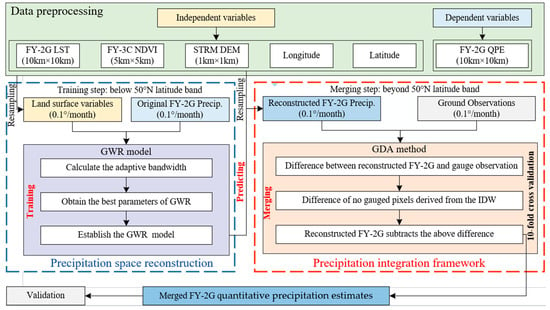
Figure 2.
Flowchart of the precipitation space reconstruction approach for the FY-2G QPE proposed in this study.
- (1)
- Data resampling. Given that the spatial resolution of FY-2G QPE is 0.1° × 0.1°, to fully utilize the relationship between the LSC variables and FY-2G QPE, it is necessary to spatially match the 5 km spatial resolution of FY-3C NDVI with FY-2G QPE. In this study, the method of cumulative averaging is used to spatially resample the FY-3C NDVI. As for DEM, this study employs the nearest-neighbor interpolation method to resample DEM data to the spatial resolution of 0.1° × 0.1°.
- (2)
- Model training. The calculation of bandwidth and kernel function is a crucial step in training the GWR model. In this study, the GWR algorithm was implemented using the “GWmodel” package in the R programming language. The “GWmodel” package offers two primary parameters for the GWR model, i.e., bw (bandwidth) and gweight (kernel function). To determine the optimal bandwidth value, an adaptive approach was employed. The optimization process was guided by the AIC value, where the goal was to minimize the AIC. In this study, a widely used Gaussian kernel function was selected for modeling purposes. Once the optimal bandwidth was determined, the GWR model for FY-2G QPE within the training area was established.
- (3)
- Precipitation reconstruction. By inputting the LSC factors from the prediction area into the final GWR model established within the training area, the reconstructed FY-2G QPE for the target area can be computed. Specifically, the NDVI, LST, DEM, and location information (longitude and latitude) are used as explanatory variables in the reconstruction model.
- (4)
- Merging correction. The GDA method is used for the fusion correction of the reconstructed results. Firstly, the reconstructed FY-2G QPE is subtracted from the ground observation to obtain the rainfall error at the station locations. The IDW interpolation method is used to estimate the rainfall error at locations outside the stations. Then, these two sets of error values are combined to obtain the complete rainfall error values within the prediction area. Finally, the reconstructed FY-2G QPE is corrected by subtracting the corresponding rainfall error values. It is worth noting that in the actual calculations, this study uses a 10-fold CV approach to compute the rainfall errors, to ensure that the validation data are mutually independent. The IDW algorithm in this study is implemented based on the “gstat” algorithm package in the R language. Similarly, the GDA method is also implemented and compiled in R language.
This study adopts the IDW method to obtain rainfall differences at ungauged grid cells through the following steps:
- (1)
- Data preparation. Gather the rainfall differences between the ground observation points, the reconstructed precipitation data, and the geographical coordinates at the gauged grid cell, including longitude and latitude.
- (2)
- Grid generation. Determine the spatial area that needs interpolation and create a regular grid covering the entire region. These grid cells will serve as the basis for the interpolated continuous surface.
- (3)
- Distance calculation. Calculate the distances between grid cells without stations and observation stations.
- (4)
- Weight allocation. Assign weights to each ungauged grid cell based on their distances and weight parameters. Closer gauged grid cells typically have higher weights, while more distant gauged grid cells have lower weights.
- (5)
- Interpolation calculation. Calculate the estimated rainfall differences for ungauged locations based on the rainfall differences at gauged grid cells and their respective weights.
- (6)
- Create a continuous Surface. Using the interpolation calculations, generate an estimate for each ungauged grid cell, thereby creating a continuous surface of rainfall differences.
For the rainfall differences at gauged grid cells, this study obtained them using a 10-fold CV method. The implementation steps are the same as described above, and after repeating this process ten times, the rainfall differences at all station locations were obtained.
3.6. Evaluation Method
To accurately measure the performance of the reconstruction results, this study adopted the three widely used statistical indicators for evaluation [60]: Correlation Coefficient (CC) could describe the agreement between reconstructed precipitation estimates and rain gauges, and the optimal value is 1. The Root Mean Square Error (RMSE) represents the error magnitude between reconstructed precipitation estimates and rain gauges, and the optimal value is 0. The Relative BIAS can provide the degree of systematic bias of reconstructed precipitation estimates, and the optimal value is 0.
Among them, refers to the baseline (rain gauges) and is the average of the baseline, and mean the reconstructed precipitation estimates and their average, refers to the number of samples.
3.7. Rainfall Anomaly Index
The Rainfall Anomaly Index (RAI) is an indicator used to measure the deviation in rainfall in a region from its long-term average [61,62]. It is commonly employed for the analysis and monitoring of climatic and meteorological variations, particularly in cases related to droughts and inadequate rainfall. The RAI was computed for a monthly period using Equations (12) and (13):
Among them, P is the current monthly rainfall for reconstructed QPEs, satellite-based QPEs or ground observations; is the monthly average precipitation of historical series for this precipitation products. The precipitation data are sorted in descending order, is the average of highest rainfall values in the top ten; is the average of lowest month rainfall values in the bottom ten. denotes the positive anomaly or negative anomaly based on positive or negative values.
The RAI can take on positive or negative values, depending on whether the actual rainfall is higher or lower than the average. Positive values indicate that actual rainfall exceeds the average, while negative values signify that actual rainfall falls below the average. The RAI can analyze climate patterns and long-term meteorological trends, such as precipitation. The RAI is also especially valuable for drought monitoring. When the RAI reflects negative values, it indicates insufficient rainfall, signaling the potential onset of drought.
4. Results
4.1. Determine the Lagging Time of NDVI Response to Precipitation
Because the monthly FY-3C NDVI is one of the crucial explanatory variables in the reconstruction model, this study conducts the spatial reconstruction of FY-2G QPE at a monthly scale. Some studies have suggested that NDVI response to precipitation has varying lag response times in different areas, and the time of NDVI response to precipitation may be as long as 2–3 months [45,46]. Hence, determining the lag response time of the FY-3C NDVI to the FY-2G QPE is essential before establishing the precipitation reconstruction model.
This study analyzes the correlation between monthly precipitation and vegetation index, based on FY-2G QPE and FY-3C NDVI. Figure 3 displays the spatial distribution of the correlation between FY-2G QPE and FY-3C NDVI in the Songliao River Basin from December 2015 to November 2019, with different latency times: (a) no monthly latency time; (b) one-month latency time; (c) two-month latency time; (d) three-month latency time. From Figure 3, there are significant variations in CC values between FY-3C NDVI and FY-2G QPE in most parts of the Songliao River Basin, with a positive correlation between precipitation and vegetation index. Among the different latency times, the FY-3C NDVI with a one-month lag exhibits the highest CC value with FY-2G QPE across the entire training area. The FY-2G QPE and FY3C NDVI exhibit higher CC values in the northern part of the Songliao River Basin than in the southern region when the lagging time is zero months. If their correlations between them are weakened, it can potentially introduce outliers during the reconstruction model training process, making it unfavorable for the reconstruction results. As the delay time increases beyond one month, the CC between NDVI and precipitation gradually decreases in the Songliao River Basin, which exhibits significant differences. When the lagging time reaches two months, there is little to no significant correlation between FY-3C NDVI and FY-2G QPE in some areas, which is unfavorable for reconstructing precipitation. Therefore, this study concludes that the response time of the FY-3C NDVI to FY-2G QPE is one month in the precipitation reconstruction model.
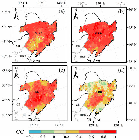
Figure 3.
Spatial distributions of CC between FY-3C NDVI in different latency times and FY-2G QPE at monthly scale over Songliao River Basin: (a) with a latency of 0 month; (b) with a latency of 1 month; (c) with a latency of 2 months; (d) with a latency of 3 months.
4.2. Performance of Fitting Precipitation
Figure 4 shows the comparison results of the overall consistency metrics for two fitted QPEs derived from GWR and RF, as well as the original FY-2G QPE and PERSIANN-CCS in the training area. Compared with the original FY-2G QPE, the accuracy of the fitted FY-2G QPEs based on RF and GWR has been greatly improved. This suggests that this study using these two methods for reconstructing FY-2G QPE in the prediction area is feasible. The assessment results show that RF and GWR approaches can significantly reduce the systematic negative BIAS of the original FY-2G QPE in that the BIAS decreases from −14.62% before adjustments to 3.56% and 3.90%, respectively. Besides BIAS, RF shows a slight increase of 5.55% in CC relative to the original FY-2G QPE, and its RMSE decreased by only 1.7%. Compared to RF, the GWR-based QPE significantly improves the consistency with ground observations relative to the original FY-2G QPE, with the highest CC value and lowest RMSE value among the three precipitation datasets. Specifically, the CC of the original FY-2G QPE has a dramatic increase of 21.46%, and the RMSE has a dramatic drop of 11.79% after fitted by the GWR model. From the fitted QPE, the GWR-based reconstructing algorithm could provide more accurate precipitation datasets than RF in the training area, which indicates the significance of adopting the GWR method to illustrate the spatially non-stationary relationship between precipitation and LSC factors [42].
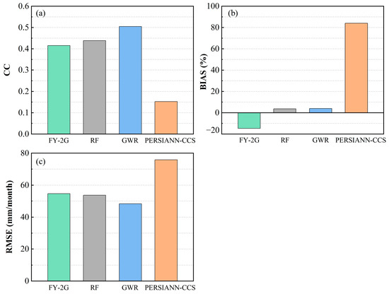
Figure 4.
Distributions of continuous metrics of FY-2G, PERSIANN-CCS, and two fitted precipitation products against the CMPA over Songliao River Basin: (a) CC, (b) BIAS, (c) RMSE.
Among the four precipitation products, PERSIANN-CCS exhibits larger rainfall errors within the Songliao River Basin compared to the original FY-2G QPE and fitted QPEs, with the lowest CC values and the highest RMSE and BIAS values. While both PERSIANN-CCS and FY-2G QPEs are precipitation retrieval based on infrared data, the overall performance of the original FY-2G QPE significantly outperforms PERSIANN-CCS over the Songliao River Basin. This is possibly due to the merging of ground observations during the data production process in terms of FY-2G QPE. Compared to PERSIANN-CCS, the performance of fitted FY-2G QPE using RF and GWR is exceptional, indicating that the accuracy of the reconstructed FY-2G QPEs in this region is not worse than this internationally recognized precipitation product. On the other hand, in the study area below 50°N, it is easy to see that the original FY-2G QPE had noteworthy negative BIAS. Meanwhile, RF and GWR effectively diminished such underestimation, suggesting the systematic negative BIAS of the original FY-2G QPE was effectively removed after they were adjusted by the RF and GWR approaches. The underestimation of the original FY-2G QPE is possibly attributed to two reasons: firstly, the FY-2G QPE is derived from a single satellite, and it is only generated from infrared information. The poor performance of FY-2G QPE could primarily result from increased snowfall in the Songliao River Basin. Although FY-2G QPE merged gauge observations in the generation step, less rain gauge data was merged in this product over Northeast China [25]; secondly, there are more missing files in the hourly FY-2G QPE compared to ground observations. Despite accumulating the daily scale data into a monthly scale for this study, the quantity of hourly FY-2G QPE is not constant throughout the day (fixed at 24).
4.3. Overall Performance of Reconstructed Precipitation
Taylor diagrams (Figure 5) are presented to compare the monthly average precipitation of three reconstructed products (RF, GWR, and PSR2G) with ground observations. Figure 5 shows that the GWR outperforms RF when only land surface environmental variables are used for reconstruction. However, after the GDA merging process, the PSR2G significantly improves the consistency metric of the GWR-based QPE. Although the standard deviation of RF is the lowest, the PSR2G is closer to ground observation than GWR in terms of the centered Root Mean Square Difference (RMSD) and CC. The PSR2G exhibits the lowest RMSD value among the three reconstructed QPEs, reducing by 26.48% compared to GWR. Additionally, the overall CC values of reconstructed precipitation obtained a remarkable improvement after adjustment by the proposed algorithm. The PSR2G with the highest CC value outperforms GWR by increasing 54.59%. These results indicate that the accuracy of the precipitation reconstruction model is significantly improved by introducing the GDA-based error correction algorithm. Furthermore, the results demonstrate that PSR2G outperforms traditional methods in terms of consistency with ground observations in Northeast China. In conclusion, PSR2G is more suitable for reconstructing the FY-2G QPE than RF and GWR in Northeast China.
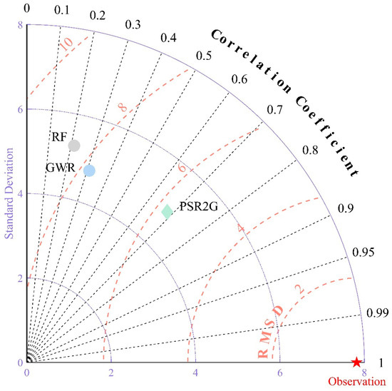
Figure 5.
Taylor diagram of monthly average precipitation for three reconstituted QPEs against CMPA over Northeast China.
4.4. Spatial Performance of Reconstructed Precipitation
Figure 6 illustrates the spatial distribution of the consistency metrics of the three reconstructed QPEs relative to CMPA in Northeast China. The comparison results of traditional methods show that GWR outperforms RF, indicating that the GWR algorithm can effectively reconstruct FY-2G QPE in areas without the FY-2G satellite coverage. Although RF and GWR have similar spatial distributions in terms of CC values, GWR has significantly higher CC values at most rain gauges than RF, particularly in the southern and northern regions. This suggests that even incorporating geographic location as an independent variable to establish the relationship with precipitation, the RF algorithm did not significantly improve the consistency between reconstructed precipitation and ground observations compared to the GWR model, which considers spatially non-stationary relationships. As for the BIAS, the spatial distribution of reconstructed QPEs based on RF and GWR is also similar, but GWR has lower BIAS values in the central and northern parts of the study area than RF. Moreover, we found that both GWR and RF have overestimations at the same rain gauges. One possible explanation for this result is that the reconstruction models based on RF and GWR fail to adequately describe the relationship between LSC factors and precipitation at such gauge stations in areas of high latitudes. Regarding the RMSE, it is evident that GWR outperforms RF in most parts of the study area. The RMSE values of GWR at most stations are less than 30 mm/month, indicating that the reconstructed QPEs based on the GWR model have lower rainfall errors than RF. In short, it further highlights that GWR could deal greatly with the influence of spatial heterogeneity between precipitation and LSC factors for the reconstruction of monthly FY-2G QPE.
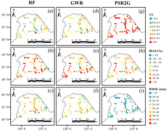
Figure 6.
Spatial distributions of temporal continuous metrics for three reconstituted QPEs against the CMPA over Northeast China: RF (a–c), GWR (d–f), PSR2G (g–i).
Compared with the reconstructed QPEs based on traditional methods, the proposed PSR2G, which was corrected by the GDA merging framework, significantly improved the consistency metrics of GWR in the spatial pattern. In terms of the CC, the PSR2G obviously outperformed RF and GWR on most gauge stations, with CC values exceeding 0.9. Regarding the BIAS, PSR2G was effective in mitigating the overestimation of GWR in the southeast and western regions, suggesting the PSR2G approach is successful in correcting such a systematic overestimation of GWR and will still be very effective in reducing the BIAS. Moreover, the PSR2G also had an obvious improvement of RMSE almost throughout the entire study area, with RMSE values below 20 mm/month in most stations, indicating that the reconstructed QPE based on the GDA method effectively reduced the RMSE of the estimated QPE by GWR. Based on the aforementioned results, PSR2G exhibits superior performances for reconstructing FY-2G QPE in Northeast China. To be specific, the merging correction method based on GDA and IDW significantly enhances the accuracy of the reconstructed precipitation from the traditional algorithm, bringing it closer to the ground observations compared to RF and GWR.
4.5. Temporal Performance of Reconstructed Precipitation
Boxplots of evaluation metrics for three reconstructed QPEs compared to CMPA in different seasons are plotted to conduct the temporal validation, as shown in Figure 7. Overall, PSR2G significantly outperforms the other two reconstructed QPEs in most seasons. In terms of CC, the RF-based reconstructed QPE has higher CC values than GWR in summer and winter, but significantly lower CC values in spring and autumn. However, PSR2G significantly improves the correlation between GWR and ground observations in all seasons, which is consistent with the spatial distribution. With respect to the BIAS, RF and GWR exhibit similar characteristics, they overestimate the precipitation in spring and summer and underestimate the precipitation in autumn and winter. From Figure 7b, the degree of overestimation and underestimation of the reconstructed FY-2G QPE by GWR is significantly lower than RF in almost all seasons. Relative to the reconstructed QPEs based on traditional methods, PSR2G effectively reduces the systematic BIAS of GWR in all seasons. Additionally, except for winter, the performance of the GWR-based reconstructed QPE is superior to RF in most seasons. As for RMSE, the GWR precipitation product has lower RMSE values than RF in most seasons, indicating that the GWR algorithm can alleviate seasonally-related rainfall errors to some extent. Meanwhile, PSR2G significantly reduces the RMSE values of GWR-based reconstructed FY-2G QPE in almost all seasons, especially in the rainy summer season.
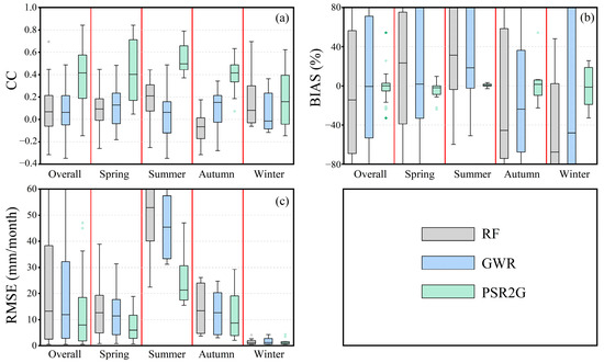
Figure 7.
Boxplots of spatial continuous metrics for three reconstituted QPEs against the CMPA in four seasons over Northeast China: (a) CC, (b) BIAS, (c) RMSE.
Based on the performance in different seasons, it can be seen that PSR2G QPE significantly improves the performance of GWR-based reconstruction results in all seasons. However, although the accuracy of GWR has been improved after the GDA merging correction process, there is still room for further improvement in its performance in winter relative to other seasons. This is possibly due to the following reason: In cold seasons, satellite precipitation data often contains considerable missed precipitation and false precipitation events at a monthly scale. As the dependent variable during the training period of the reconstruction model in the Songliao River Basin below 50°N, the FY-2G QPE inevitably introduces rainfall errors and uncertainties into the reconstructed results. Additionally, this also leads to a significant reduction in the number of grid cells with stations during the winter, further reducing the available sample number. On the other hand, we speculate that insufficient response of some land surface environmental variables to precipitation during the winter is also an important reason.
4.6. Temporal Analysis of Precipitation Anomalies
Figure 8 depicts the temporal distribution of RAI values derived from four QPEs and CMPA and overall CC values in terms of the RAI values from these QPEs against CMPA at a monthly scale over the Songliao River Basin. When RAI > 0, it indicates that the rainfall is above the average level, making it more susceptible to flooding. When RAI < 0, it signifies insufficient rainfall, which can lead to drought conditions. Based on ground observations, the months of July 2016–2017 had the highest RAI values, with August following closely behind. Similarly, in 2018 and 2019, August recorded the highest RAI values, with July as the next in line. This suggests that July and August are the rainiest months in the region. Conversely, January to March and November to December in the years 2016–2019 were consistently characterized as dry months, indicating lower precipitation during the cold season. In the comparison of satellite-based QPEs, we found that the RAI curve of the original FY-2G closely aligns with ground observations. For instance, the original FY-2G RAI also detected drought months from January to March and November to December, which is consistent with ground observations. Similarly, the RAI curve of the fitted FY-2G QPEs closely resembles that of the original FY-2G, with RAI values remarkably consistent with ground observations. Furthermore, from Figure 8b, it is evident that the fitted GWR precipitation product’s RAI exhibited the highest CC values with ground observation RAI, followed by RF, both slightly outperforming the original FY-2G. This implies that this reconstruction method accurately captures variations in precipitation and maintains a high level of consistency with the original FY-2G QPE in simulating rainfall patterns. It is worth noting that PERSIANN-CCS demonstrated poorer performance than other QPEs. While it did detect some rainy months, it frequently misclassified drought months as rainy, resulting in a higher false alarm rate. This discrepancy is also reflected in its RAI and has the lowest CC value with ground observation RAI, which is less than 0.3. As a precipitation product based on infrared data retrieval, the performance of PERSIANN-CCS is significantly worse than the original FY-2G and even the fitted precipitation products, exhibiting a substantial difference in RAI values compared to ground observations. This suggests that PERSIANN-CCS faces challenges in accurately capturing and detecting rainfall patterns related to both wet and dry conditions, requiring further refinement and calibration.
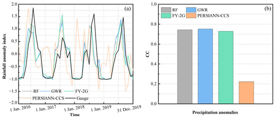
Figure 8.
(a) Temporal distribution of RAI values derived from fitted QPEs, satellite-based QPEs and CMPA over the Songliao River Basin; (b) Overall CC values in terms of the RAI values from these QPEs against CMPA at a monthly scale over the Songliao River Basin.
Figure 9 depicts the temporal distribution of RAI values derived from four QPEs and CMPA and overall CC values in terms of the RAI values from these QPEs against CMPA at a monthly scale in Northeast China. The ground observations from May to September 2016 to 2019 have positive RAI values, except for the RAI values of the ground observations from May to June 2018 are negative, which are slightly lower than 0. This indicates that for areas with a latitude band beyond 50°N over the Songliao Basin, May to September seems to be the rainy season, while the other months typically experience dry conditions. Similar to the performance in the training area, the RAI values of PERSIANN-CCS exhibited almost no significant correlation with the RAI values of ground observations in the prediction region. Precipitation anomalies reconstructed using RF and GWR are significantly closer to ground observations than PERSIANN-CCS, with their CC values exceeding 0.8. Additionally, precipitation anomalies of GWR outperform RF in terms of RAI. However, although temporal trends of the RAI values derived from purely reconstructed QPEs are consistent with ground observations, they still have significant differences in their numerical values for RAI. For example, in August 2016, the ground observations yielded a positive RAI value of 0.631, while the RAI values calculated by RF and GWR were −0.191 and 0.002, respectively. In September of the same year, the ground observations yielded a positive RAI value of 1.092, while the RAI values from RF and GWR were negative at −0.101 and −0.03, respectively. From these results, while precipitation anomalies of GWR are closer to the ground observations than RF, it still occasionally misclassifies rainy months as dry months. After fusion correction, the RAI of PSR2G in August and September 2016 is 0.575 and 1.059, respectively, which not only reduces the phenomenon of false alarm events but also the calculated RAI values are closer to ground observations than RF and GWR. This demonstrates that PSR2G can significantly improve the performance of GWR in detecting rainy and dry conditions by calculating precipitation anomalies.
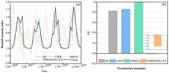
Figure 9.
(a) Temporal distribution of RAI values derived from reconstructed QPEs, satellite-based QPEs and CMPA in Northeast China; (b) Overall CC values in terms of the RAI values from these QPEs against CMPA at a monthly scale in Northeast China.
5. Discussion
5.1. Sensitivity Analysis of the Proposed Algorithm to the Size of the Prediction Area
From the fundamental formula of GWR, the modeling process involves using LSC factors as explanatory variables and FY-2G QPE as the response variable by training in adjacently spatial locations. The trained model is then applied to nearby LSC data to predict the precipitation estimate. It should be noted that the distance between the prediction area and the training area may affect the prediction results.
Figure 10 shows the spatial distribution of different prediction regions over Northeast China. The different numbers of prediction areas actually represent the number of times that the data needs to be predicted. For example, a partition number of 2 means that the prediction area above 50°N in the Songliao River Basin is divided into two parts (Figure 10b), 1 and 2. First, the GWR model is trained on the training area below 50°N, and the independent variable data of prediction area 1 is used as input for prediction using the built model. After the precipitation data in area 2 is predicted, the independent variable data and predicted precipitation data in area 1 are integrated with the training data and retrained. Finally, the independent variable data of prediction area 2 is used as input into the rebuilt model for prediction. As the number of prediction areas increases, it indicates that the prediction area is getting closer to the training area.
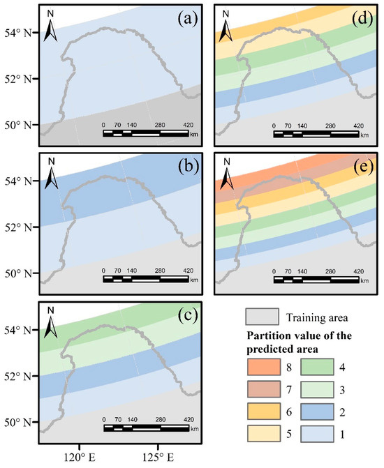
Figure 10.
Spatial distribution of different prediction region over Northeast China: (a) 1 partition, (b) 2 partitions, (c) 4 partitions, (d) 6 partitions, (e) 8 partitions.
To better analyze the influence of the distance between the prediction area and the reconstruction results, this study plots the performance of GWR and PSR2G under different prediction areas in Figure 11. From Figure 11, we can see at least three pieces of information: Firstly, the accuracy indicators of GWR show significant variations for different numbers of prediction areas, indicating that the GWR model is highly sensitive to the position of the prediction area. Secondly, as the number of prediction areas increases from 1 to 8, suggesting that the prediction area is getting closer to the training area, the accuracy of GWR improves gradually, especially for CC and RMSE. The GWR exhibits the highest CC value and the lowest RMSE value when the number of prediction areas is 8, further validating that the GWR model is sensitive to the position variations of the prediction area. It suggests that as the distance between the training and prediction regions decreases, the density of the encompassed sample during model training also rises in training regions. The precipitation and LSC factors have a stronger spatial correlation in such regions, resulting in land surface environmental data to explain precipitation yields superior performance. Finally, under different subregion numbers, PSR2G significantly improved the performance of GWR, as shown by PSR2G having higher CC, lower BIAS and RMSE than GWR, especially when the subregion number of 8. This also suggests that the improvement of PSR2G over GWR accuracy is also dependent on the accuracy of the original data.

Figure 11.
Distributions of continuous metrics for the two GWR-based reconstituted QPEs against the CMPA in different prediction region over Northeast China.
5.2. Strengths of the Proposed Method
GWR-based reconstruction QPE has demonstrated its capability in generating finely accurate datasets. It is noted that the spatial heterogeneity in the connections between precipitation and LSC factors is prevalent [63]. To address the challenge of spatial heterogeneity, the GWR model was proposed to capture the intricate connections between precipitation and LSC factors by local regression analysis [42]. Unlike conventional approaches that assume constant spatial relationships between precipitation and environmental variables during the reconstruction process, GWR takes into account the spatial variability of these relationships [26,29,33]. This enables GWR to provide a spatially adaptive reconstruction, resulting in enhanced accuracy and applicability of the reconstructed precipitation data. Consequently, considering the effectiveness of GWR in downscaling satellite-derived precipitation data becomes evident, warranting its selection for the spatial reconstruction of FY-2G QPE in the current investigation.
Satellite-based precipitation estimates provide notable benefits in capturing precipitation changes with high precision in both space and time, particularly in regions where ground-based rain gauges are limited [44]. Nonetheless, these products being indirect estimations of precipitation, inherently encompass systematic biases and random errors that stem from regional, seasonal, and diurnal scales [44,64]. For the GWR-based precipitation reconstruction model, the FY-2G QPE as a crucial response variable, results in reconstructed precipitation still introducing intrinsic errors and uncertainty inherited from the FY-2G QPE. Some research studies indicate that these rainfall errors can be effectively mitigated by incorporating ground-based observations, thus enhancing the accuracy of satellite-only precipitation estimates [17]. Hence, a precipitation space reconstruction algorithm based on GWR coupled with GDA was developed in this study, to reconstruct and calibrate FY-2G QPE in the coverage miss area. Table 1 shows the overall consistency metrics for three reconstructed QPEs and PERSIANN-CCS in Northeast China and the original FY-2G QPE in the training area. In general, the PSR2G QPE performs the best among the three reconstructed FY-2G QPEs, followed by GWR, and then RF. The accuracy of the reconstructed results after merging correction is better than those before merging correction, which manifests that the GDA algorithm has significantly contributed to the advancement of the estimated FY-2G QPE from the GWR model. Furthermore, relative to original FY-2G QPE in adjacent areas (the latitude band of the Songliao River Basin below 50°N), the performance of three reconstructed QPEs outperforms the original FY-2G QPE, particularly with PSR2G. This suggests that the reconstructed QPEs based on these three methods did not compromise the accuracy of the original FY-2G QPE. It is worth noting that the existing global satellite precipitation product, PERSIANN-CCS, exhibits a performance in the study region that closely mirrors its performance in the training area. It is unsatisfactory that it still has the worst performance among the five products. Even the reconstructed products, including RF and GWR before merging, outperform PERSIANN-CCS. This indicates the reasonableness and effectiveness of the research approach and findings presented in this study.

Table 1.
The continuous metrics of the original FY-2G QPE, PERSIANN-CCS and three reconstituted precipitation products against the CMPA in this study.
The PSR2G retains the advantages GWR model to adaptively account for variations in relationships across different geographical locations, leading to a more accurate depiction of how precipitation and LSC factors interact. Furthermore, another advantage of the PSR2G is that the incorporation of ground observations and the GDA algorithm has significantly contributed to reducing rainfall errors for the reconstructed precipitation data. This is also consistent with the previous assessment results that the PSR2G is the more suitable method for reconstructing FY-2G QPE than RF and GWR in Northeast China. The PSR2G approach can provide high-quality precipitation datasets over the lost coverage of the satellite precipitation estimates, and estimated results hold practical utility for hydrological and meteorological investigations.
5.3. Sources of Uncertainty and Future Research
The results mentioned above have validated the effectiveness of the precipitation reconstruction methods employed in this study; nevertheless, there remain certain uncertainties that could potentially lead to systematic and random errors within the reconstructed precipitation datasets.
Based on the FY-2G QPE and explanatory variables over Songliao River Basin with a latitude band below 50°/N, this study adopts the proposed PSR2G algorithm to reconstruct FY-2G QPE with a spatiotemporal resolution of 0.1°/month over Northeast China. However, because the spatial resolution of some explanatory variables does not match the FY-2G QPE, this study adopts the accumulative average method to resample the resolution by neighboring gird. This process could lead to a loss of intricate details within these variables, particularly in regions of complex topography such as mountains [40,42]. Hence, in order to prevent the introduction of new error sources during the data resampling process, it is crucial to take a comprehensive approach by considering both the spatial scale and the matching method when choosing data of different spatial resolutions.
Further research is essential to explore optimal strategies for selecting the most appropriate set of explanatory variables. It is important to note that some unused LSC factors also possess the capability to present the spatial distribution of precipitation, thus potentially enriching the precision of reconstructed precipitation [36]. Wang et al. [40] pointed out that some LSC elements like relief, aspect, slope, surface roughness, and humidity are studied as having crucial roles in the downscaling precipitation. However, our current study restricts its focus exclusively to latitude, longitude, altitude, LST, and NDVI overlooking these supplementary variables. Moreover, in this study, only LSC products were investigated as the auxiliary variable to reconstruct the FY-2G precipitation data. It is noted that some atmospheric variables are also strongly related to the spatial distribution of precipitation, such as cloud-top temperature. Considering this, it is hopeful to utilize these atmospheric variables to reconstruct satellite precipitation estimates in regions lacking satellite coverage.
Precipitation fusion is an effective tool for producing improved precipitation data by combining gauge and satellite observations [43,58]. However, the accuracy and number of rain observations are crucial in affecting the performance of fusion results. It is worth noting that gauge measurements still exist with systematic errors, which include wind-induced undercatch, wetting loss, evaporation loss, and the underestimation of trace precipitation [40]. The great BIAS may appear in cold regions characterized by elevated latitudes and altitudes, as was previously documented by Wang et al. [40]. The reconstructed precipitation data in this study is located in such areas. We noted that in the study region with a total area of 175,546 km2; only 80 ground-based rain gauges were adopted to merge reconstructed FY-2G QPE and ground observations over the study region [30]. It means that per ground-based observation station represents an area exceeding 2000 km2. Furthermore, the ground stations are distributed unevenly over the study region, most concentrated in the eastern regions while sparsely covering the western and northern areas, which suggests that the ground-based rain gauges cannot sufficiently represent the spatial pattern of precipitation over the entire study region. Hence, the quality of reconstructed precipitation data coupled with sparse ground observation data inevitably limits the GDA methods in the PSR2G procedure for improving GWR results, which is consistent with the conclusion of Duan and Bastiaanssen [29]. Li et al. [65] have demonstrated that augmenting the density of the gauge network can indeed enhance the quality of fused products.
Satellite-derived precipitation exhibits worse performance during the colder months [36,66]. While the reconstructed precipitation through PSR2G represents a notable enhancement over previous methods like GWR and RF, its improvement during the cold season remains unsatisfactory. Hence, the reconstruction and fusion correction of satellite-derived precipitation data during these colder periods hold significant importance. Given this, further refinement and advancement of this algorithm are necessary for subsequent studies.
6. Conclusions
Limited by observation coverage of Fengyun-based satellite-borne sensor, at present, the obtained FY-2G QPE are still missing over Northeast China. In this study, a precipitation space reconstruction based on GWR coupled with GDA (PSR2G) was developed, to reconstruct and calibrate FY-2G QPE over Northeast China at a monthly scale from December 2015 to November 2019. The reconstructed precipitation products were compared to the ground observations to assess its temporal-spatial performance. The major conclusions of this study are summarized as follows:
- The relationship between monthly FY-2G QPE and FY-3C NDVI highlights significant lagging times in the response of NDVI to precipitation. The results showed that the highest correlation between FY-2G QPE and FY-3C NDVI in the Songliao River Basin was achieved when the lagging time was one month, and FY-2G QPE and FY-3C NDVI had no correlation in most areas of the Songliao River Basin when the lagging time was three months. Therefore, we determined that the NDVI response time to precipitation for the reconstruction model is one month.
- From the assessment results for fitted QPEs, the CC values of the fitted FY-2G QPEs derived by GWR and RF were significantly improved compared to the original FY-2G QPE in the study area with a latitude below 50°N, and the BIAS and RMSE values were also significantly reduced, with GWR outperforming RF. As For the reconstructed results, it is noted that the accuracy of the GWR model, which considers spatial non-stationarity, is still better than that of RF. This further demonstrates that the GWR method could more accurately describe the relationship between land surface environmental variables and precipitation than RF in Northeast China.
- Statistical evaluation revealed that the PSR2G QPE has the highest accuracy in estimating precipitation in regions where FY-2G satellite coverage is lost among the three reconstructed products, followed by GWR and RF. The performance of reconstruction precipitation after the merging correction is significantly superior to the only reconstructed precipitation product. This also indicates that GDA algorithms successfully reduced the rainfall errors of the GWR QPE by introducing ground observations, which further improves the consistency of the reconstructed QPE with ground observation.
- Comparison of GWR QPE based on the slide prediction in different subregions with gauged data showed that the GWR QPE has a higher performance as the distances between the prediction area and the training area were closer. The increase in sample numbers in the training area may also be responsible for the GWR QPE has better performance than other subregions when the number of slide predictions is maximum. Although the accuracy of GWR QPE exists instability, PSR2G presents similar behaviors, in which such results from short-distance prediction have the highest accuracy while long-distance prediction has the worst accuracy. This means that the accuracy of PSR2G QPE still depends on the performance of the original data even if PSR2G significantly improves the performance of GWR.
Author Contributions
Conceptualization, H.W.; methodology, H.W.; software, H.W.; validation, H.W. and Z.S.; formal analysis, H.W.; resources, H.W.; writing—original draft preparation, H.W.; writing—review and editing, B.Y., H.W. and Z.S.; visualization, H.W.; funding acquisition, B.Y., Z.S. and H.W. All authors have read and agreed to the published version of the manuscript.
Funding
This work was sponsored by the National Natural Science Foundation of China (U2243229, 42301385).
Acknowledgments
The authors are grateful to the NMIC of CMA for providing ground observation data, and thankful to NSMC for providing FY-2G QPE, FY-2G LST and FY-3C NDVI, and also thankful to Resource and Environment Science and Data Center of Chinese Academy of Sciences for providing DEM.
Conflicts of Interest
The authors declare no conflict of interest.
References
- Hou, A.; Kakar, R.; Neeck, S.; Azarbarzin, A.; Kummerow, C.; Kojima, M.; Oki, R.; Nakamura, K.; Iguchi, T. The Global Precipitation Measurement Mission. Bull. Am. Meteorol. Soc. 2014, 95, 701–722. [Google Scholar] [CrossRef]
- Michaelides, S.; Levizzani, V.; Anagnostou, E.; Bauer, P.; Kasparis, T.; Lane, J.E. Precipitation: Measurement, remote sensing, climatology and modeling. Atmos. Res. 2009, 94, 512–533. [Google Scholar] [CrossRef]
- Zhai, P.; Zhang, X.; Wan, H.; Pan, X. Trends in total precipitation and frequency of daily precipitation extremes over China. J. Clim. 2005, 18, 1096–1108. [Google Scholar] [CrossRef]
- Kidd, C.; Becker, A.; Huffman, G.J.; Muller, C.L.; Joe, P.; Skofronick-Jackson, G.; Kirschbaum, D.B. So, how much of the Earth’s surface is covered by rain gauges? Bull. Am. Meteorol. Soc. 2017, 98, 69–78. [Google Scholar] [CrossRef] [PubMed]
- Shen, Z.; Yong, B.; Gourley, J.J.; Qi, W.; Lu, D.; Liu, J.; Ren, L.; Hong, Y.; Zhang, J. Recent global performance of the Climate Hazards group Infrared Precipitation (CHIRP) with Stations (CHIRPS). J. Hydrol. 2020, 591, 125284. [Google Scholar] [CrossRef]
- Zhou, Z.; Yong, B.; Liu, J.; Liao, A.; Wang, N.; Zhu, Z.; Lu, D.; Li, W.; Zhang, J. Preliminary evaluation of the hobo data logging rain gauge at the Chuzhou hydrological experiment station, China. Adv. Meteorol. 2019, 2019, 5947976. [Google Scholar] [CrossRef]
- Wen, X.; Ma, X.; Zhang, C.; Zheng, S. Comparative study of piezoelectric precipitation sensor and tipping bucket precipitation sensor. Autom. Appl. 2021, 11, 38–40+45. (In Chinese) [Google Scholar] [CrossRef]
- Fiser, O.; Wilfert, O. Novel processing of Tipping-bucket rain gauge records. Atmos. Res. 2009, 92, 283–288. [Google Scholar] [CrossRef]
- Santana, M.A.; Guimarães, P.L.; Lanza, L.G.; Vuerich, E. Metrological analysis of a gravimetric calibration system for tipping-bucket rain gauges. Meteorol. Appl. 2015, 22, 879–885. [Google Scholar] [CrossRef]
- Leeper, R.D.; Kochendorfer, J. Evaporation from weighing precipitation gauges: Impacts on automated gauge measurements and quality assurance methods. Atmos. Meas. Tech. 2015, 8, 2291–2300. [Google Scholar] [CrossRef]
- Buytaert, W.; Celleri, R.; Willems, P.; De Bievre, B.; Wyseure, G. Spatial and temporal rainfall variability in mountainous areas: A case study from the south Ecuadorian Andes. J. Hydrol. 2006, 329, 413–421. [Google Scholar] [CrossRef]
- Bournas, A.; Baltas, E. Determination of the ZR Relationship through spatial analysis of X-band weather radar and rain gauge data. Hydrology 2022, 9, 137. [Google Scholar] [CrossRef]
- Dinku, T.; Anagnostou, E.N.; Borga, M. Improving Radar-Based Estimation of Rainfall over Complex Terrain. J. Appl. Meteorol. 2002, 41, 1163–1178. [Google Scholar] [CrossRef]
- Sharif, H.O.; Ogden, F.L.; Krajewski, W.F.; Xue, M. Numerical simulations of radar rainfall error propagation. Water Resour. Res. 2002, 38, 1140. [Google Scholar] [CrossRef]
- Kidd, C. Satellite rainfall climatology: A review. Int. J. Climatol. 2001, 21, 1041–1066. [Google Scholar] [CrossRef]
- Tapiador, F.J.; Turk, F.J.; Petersen, W.; Hou, A.Y.; García-Ortega, E.; Machado, L.A.T.; Angelis, C.F.; Salio, P.; Kidd, C.; Huffman, G.J.; et al. Global precipitation measurement: Methods, datasets and applications. Atmos. Res. 2012, 104–105, 70–97. [Google Scholar] [CrossRef]
- Huffman, G.J.; Adler, R.F.; Bolvin, D.T.; Gu, G.; Nelkin, E.J.; Bowman, K.P.; Hong, Y.; Stocker, E.F.; Wolff, D.B. The TRMM Multisatellite Precipitation Analysis (TMPA): Quasi-Global, Multiyear, Combined-Sensor Precipitation Estimates at Fine Scales. J. Hydrometeorol. 2007, 8, 38–55. [Google Scholar] [CrossRef]
- Huffman, G.J.; Bolvin, D.T.; Braithwaite, D.; Hsu, K.; Joyce, R.; Xie, P. GPM Integrated Multi-Satellite Retrievals for GPM (IMERG) Algorithm Theoretical Basis Document (ATBD) Version 4.4. PPS, NASA/GSFC, 30 pp. 2014. Available online: http://pmm.nasa.gov/sites/default/files/document_files/IMERG_ATBD_V4.4.pdf (accessed on 1 December 2019).
- Kubota, T.; Shige, S.; Hashizume, H.; Aonashi, K.; Takahashi, N.; Seto, S.; Hirose, M.; Takayabu, Y.N.; Ushio, T.; Nakagawa, K.; et al. Global Precipitation Map Using Satellite-Borne Microwave Radiometers by the GSMaP Project: Production and Validation. IEEE Trans. Geosci. Remote Sens. 2007, 45, 2259–2275. [Google Scholar] [CrossRef]
- Joyce, R.J.; Janowiak, J.E.; Arkin, P.A.; Xie, P. CMORPH: A method that produces global precipitation estimates from passive microwave and infrared data at high spatial and temporal resolution. J. Hydrometeorol. 2014, 5, 487–503. [Google Scholar] [CrossRef]
- Hong, Y.; Hsu, K.; Sorooshian, S.; Gao, X. Precipitation estimation from remotely sensed imagery using an artificial neural network cloud classification system. J. Appl. Meteorol. 2004, 43, 1834–1852. [Google Scholar] [CrossRef]
- Xu, J.; Ma, Z.; Tang, G.; Ji, Q.; Min, X.; Wan, W.; Shi, Z. Quantitative Evaluations and Error Source Analysis of Fengyun-2-Based and GPM-Based Precipitation Products over Mainland China in Summer, 2018. Remote Sens. 2019, 11, 2992. [Google Scholar] [CrossRef]
- Lu, H.; Ding, L.; Ma, Z.; Li, H.; Lu, T.; Su, M.; Xu, J. Spatiotemporal Assessments on the Satellite-Based Precipitation Products from Fengyun and GPM Over the Yunnan-Kweichow Plateau, China. Earth Space Sci. 2020, 7, e2019EA000857. [Google Scholar] [CrossRef]
- Wu, H.; Yong, B.; Shen, Z.; Qi, W. Comprehensive error analysis of satellite precipitation estimates based on Fengyun-2 and GPM over Chinese mainland. Atmos. Res. 2021, 263, 105805. [Google Scholar] [CrossRef]
- Sun, Z.; Long, D.; Hong, Z.; Hamouda, M.A.; Mohamed, M.M.; Wang, J. How China’s Fengyun Satellite Precipitation Product Compares with Other Mainstream Satellite Precipitation Products. J. Hydrometeorol. 2022, 23, 785–806. [Google Scholar] [CrossRef]
- Immerzeel, W.W.; Rutten, M.M.; Droogers, P. Spatial downscaling of TRMM precipitation using vegetative response on the Iberian Peninsula. Remote Sens. Environ. 2009, 113, 362–370. [Google Scholar] [CrossRef]
- Trenberth, K.E.; Shea, D.J. Relationships between precipitation and surface temperature. Geophys. Res. Lett. 2005, 32, L14703. [Google Scholar] [CrossRef]
- Spracklen, D.V.; Arnold, S.R.; Taylor, C.M. Observations of increased tropical rainfall preceded by air passage over forests. Nature 2012, 489, 282–285. [Google Scholar] [CrossRef]
- Duan, Z.; Bastiaanssen, W.G.M. First results from Version 7 TRMM 3B43 precipitation product in combination with a new downscaling–calibration procedure. Remote Sens. Environ. 2013, 131, 1–13. [Google Scholar] [CrossRef]
- Jing, W.; Zhang, P.; Jiang, H.; Zhao, X. Reconstructing Satellite-Based Monthly Precipitation over Northeast China Using Machine Learning Algorithms. Remote Sens. 2017, 9, 781. [Google Scholar] [CrossRef]
- Schultz, P.A.; Halpert, M.S. Global analysis of the relationships among a vegetation index, precipitation and land surface temperature. Remote Sens. 1995, 16, 2755–2777. [Google Scholar] [CrossRef]
- Jia, S.; Zhu, W.; Lű, A.; Yan, T. A statistical spatial downscaling algorithm of TRMM precipitation based on NDVI and DEM in the Qaidam Basin of China. Remote Sens. Environ. 2011, 115, 3069–3079. [Google Scholar] [CrossRef]
- Fang, J.; Du, J.; Xu, W.; Shi, P.; Li, M.; Ming, X. Spatial downscaling of TRMM precipitation data based on the orographical effect and meteorological conditions in a mountainous area. Adv. Water Resour. 2013, 61, 42–50. [Google Scholar] [CrossRef]
- Eltahir, E.A.B. A Soil Moisture-Rainfall Feedback Mechanism: 1. Theory and observations. Water Resour. Res. 1998, 34, 765–776. [Google Scholar] [CrossRef]
- Brunsell, N. Characterization of land-surface precipitation feedback regimes with remote sensing. Remote Sens. Environ. 2006, 100, 200–211. [Google Scholar] [CrossRef]
- Lu, X.; Tang, G.; Wang, X.; Liu, Y.; Jia, L.; Xie, G.; Li, S.; Zhang, Y. Correcting GPM IMERG precipitation data over the Tianshan Mountains in China. J. Hydrol. 2019, 575, 1239–1252. [Google Scholar] [CrossRef]
- Zhang, Y.; Li, Y.; Ji, X.; Luo, X.; Li, X. Fine-resolution precipitation mapping in a mountainous watershed: Geostatistical downscaling of TRMM products based on environmental variables. Remote Sens. 2018, 10, 119. [Google Scholar] [CrossRef]
- Jing, W.; Yang, Y.; Yue, X.; Zhao, X. A comparison of different regression algorithms for downscaling monthly satellite-based precipitation over North China. Remote Sens. 2016, 8, 835. [Google Scholar] [CrossRef]
- Chen, C.; Zhao, S.; Duan, Z.; Qin, Z. An improved spatial downscaling procedure for TRMM 3B43 precipitation product using geographically weighted regression. IEEE J. Sel. Top. Appl. Earth Obs. Remote Sens. 2015, 8, 4592–4604. [Google Scholar] [CrossRef]
- Wang, H.; Zang, F.; Zhao, C.; Liu, C. A GWR downscaling method to reconstruct high-resolution precipitation dataset based on GSMaP-Gauge data: A case study in the Qilian Mountains, Northwest China. Sci. Total Environ. 2022, 810, 152066. [Google Scholar] [CrossRef]
- Foody, G.M. Geographical weighting as a further refinement to regression modelling: An example focused on the NDVI–rainfall relationship. Remote Sens. Environ. 2003, 88, 283–293. [Google Scholar] [CrossRef]
- Xu, S.; Wu, C.; Wang, L.; Gonsamo, A.; Shen, Y.; Niu, Z. A new satellite-based monthly precipitation downscaling algorithm with non-stationary relationship between precipitation and land surface characteristics. Remote Sens. Environ. 2015, 162, 119–140. [Google Scholar] [CrossRef]
- Chao, L.; Zhang, K.; Li, Z.; Zhu, Y.; Wang, J.; Yu, Z. Geographically weighted regression based methods for merging satellite and gauge precipitation. J. Hydrol. 2018, 558, 275–289. [Google Scholar] [CrossRef]
- Ma, Z.; Xu, J.; Zhu, S.; Yang, J.; Tang, G.; Yang, Y.; Shi, Z.; Hong, Y. AIMERG: A new Asian precipitation dataset (0.1°/half-hourly, 2000–2015) by calibrating the GPM-era IMERG at a daily scale using APHRODITE. Earth Syst. Sci. Data 2020, 12, 1525–1544. [Google Scholar] [CrossRef]
- Quiroz, R.; Yarlequé, C.; Posadas, A.; Mares, V.; Immerzeel, W.W. Improving daily rainfall estimation from NDVI using a wavelet transform. Environ. Model. Softw. 2011, 26, 201–209. [Google Scholar] [CrossRef]
- Nicholson, S.E.; Davenport, M.L.; Malo, A.R. A comparison of the vegetation response to rainfall in the Sahel and East Africa, using normalized difference vegetation index from NOAA AVHRR. Clim. Chang. 1990, 17, 209–241. [Google Scholar] [CrossRef]
- Shen, Z.; Yong, B. Downscaling the GPM-based satellite precipitation retrievals using gradient boosting decision tree approach over Mainland China. J. Hydrol. 2021, 602, 126803. [Google Scholar] [CrossRef]
- Hu, C.; Xia, J.; She, D.; Xu, C.; Zhang, L.; Song, Z.; Zhao, L. A modified regional L-moment method for regional extreme precipitation frequency analysis in the Songliao River Basin of China. Atmos. Res. 2019, 230, 104629. [Google Scholar] [CrossRef]
- Qi, J.; Song, J.; Liu, H. Characteristics of temperature and precipitation in Northeast China from 1951 to 2000. J. Meteorol. Environ. 2006, 22, 1–5. (In Chinese) [Google Scholar]
- Xu, J.; Zhang, W.; Yang, J.; Zhao, L. Practical Manual of Fengyun-2 Satellite Business Products and Satellite Data Format; China Meteorological Press: Beijing, China, 2008; pp. 11–16. (In Chinese) [Google Scholar]
- Tang, F.; Zou, X.; Yang, H.; Weng, F. Estimation and Correction of Geolocation Errors in FengYun-3C Microwave Radiation Imager Data. IEEE Trans. Geosci. Remote Sens. 2016, 54, 407–420. [Google Scholar] [CrossRef]
- Lin, Z.; Chen, F.; Niu, Z.; Li, B.; Yu, B.; Jia, H.; Zhang, M. An active fire detection algorithm based on multi-temporal FengYun-3C VIRR data. Remote Sens. Environ. 2018, 211, 376–387. [Google Scholar] [CrossRef]
- Brunsdon, C.; Fotheringham, A.S.; Charlton, M.E. Geographically weighted regression: A method for exploring spatial nonstationarity. Geogr. Anal. 1996, 28, 281–298. [Google Scholar] [CrossRef]
- Gao, Y.; Huang, J.; Li, S.; Li, S. Spatial pattern of non-stationarity and scale-dependent relationships between NDVI and climatic factors—A case study in Qinghai-Tibet Plateau, China. Ecol. Indic. 2012, 20, 170–176. [Google Scholar] [CrossRef]
- Lu, B.; Charlton, M.; Harris, P.; Fotheringham, A.S. Geographically weighted regression with a non-Euclidean distance metric: A case study using hedonic house price data. Int. J. Geogr. Inf. Sci. 2014, 28, 660–681. [Google Scholar] [CrossRef]
- Akaike, H. A new look at the statistical identification model. IEEE Trans. Autom. Control 1974, 19, 716–723. [Google Scholar] [CrossRef]
- Breiman, L. Random forests. Mach. Learn. 2001, 45, 5–32. [Google Scholar] [CrossRef]
- Shen, Z.; Wu, H. A comparative analysis of merging strategies for satellite precipitation estimates and ground observations over Chinese mainland. J. Atmos. Sol. Terr. Phys. 2023, 246, 106072. [Google Scholar] [CrossRef]
- Watson, D.F.; Philip, G.M. A refinement of inverse distance weighted interpolation. Geo-processing 1985, 2, 315–327. [Google Scholar]
- Yong, B.; Ren, L.; Hong, Y.; Gourley, J.; Tian, Y.; Huffman, G.; Chen, X.; Wang, W.; Wen, Y. First evaluation of the climatological calibration algorithm in the real-time TMPA precipitation estimates over two basins at high and low latitudes. Water Resour. Res. 2013, 49, 2461–2472. [Google Scholar] [CrossRef]
- Raziei, T. Revisiting the Rainfall Anomaly Index to serve as a Simplified Standardized Precipitation Index. J. Hydrol. 2021, 602, 126761. [Google Scholar] [CrossRef]
- Aryal, A.; Maharjan, M.; Talchabhadel, R.; Thapa, B.R. Characterizing Meteorological Droughts in Nepal: A Comparative Analysis of Standardized Precipitation Index and Rainfall Anomaly Index. Earth 2022, 3, 409–432. [Google Scholar] [CrossRef]
- Guan, H.; Wilson, J.L.; Xie, H. A cluster-optimizing regression-based approach for precipitation spatial downscaling in mountainous terrain. J. Hydrol. 2009, 375, 578–588. [Google Scholar] [CrossRef]
- Ebert, E.E.; Janowiak, J.E.; Kidd, C. Comparison of near-real-time precipitation estimates from satellite observations and numerical models. Bull. Am. Meteorol. Soc. 2007, 88, 47–64. [Google Scholar] [CrossRef]
- Li, H.; Hong, Y.; Xie, P.; Gao, J.; Niu, Z.; Kirstetter, P.; Yong, B. Variational merged of hourly gauge-satellite precipitation in China: Preliminary results. J. Geophys. Res. Atmos. 2015, 120, 9897–9915. [Google Scholar] [CrossRef]
- Tang, G.; Long, D.; Behrangi, A.; Wang, C.; Hong, Y. Exploring deep neural networks to retrieve rain and snow in high latitudes using multisensor and reanalysis data. Water Resour. Res. 2018, 54, 8253–8278. [Google Scholar] [CrossRef]
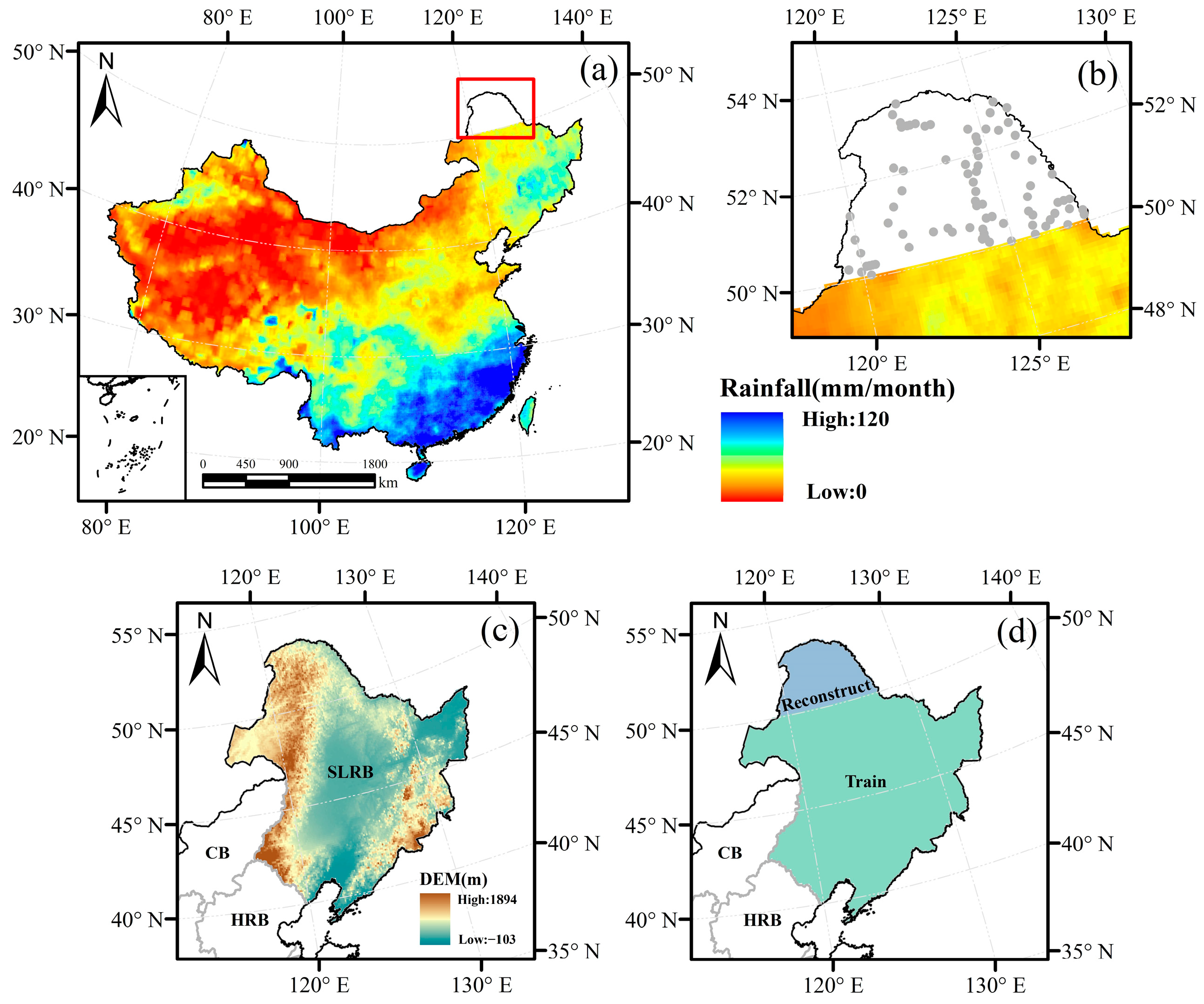
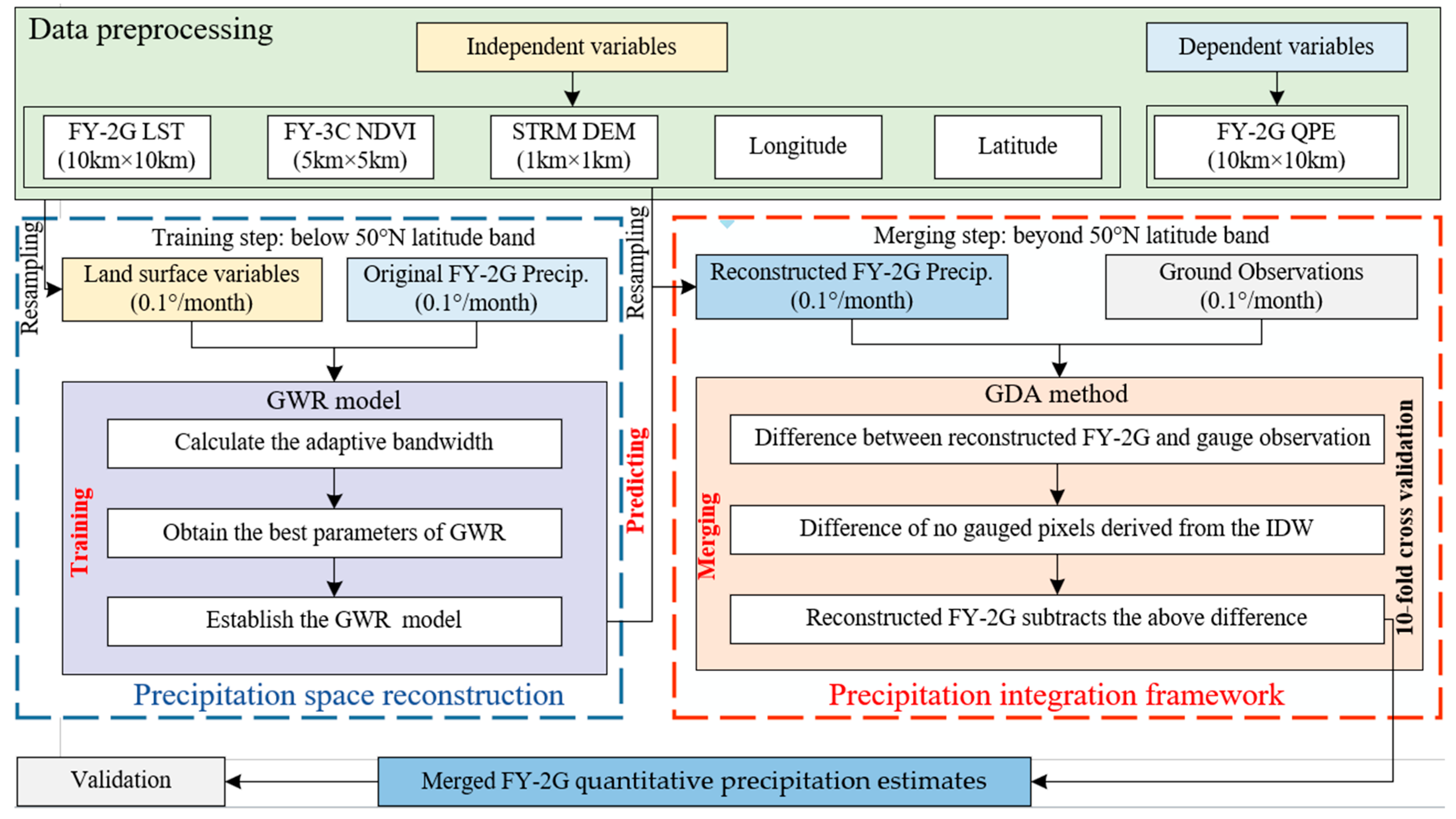
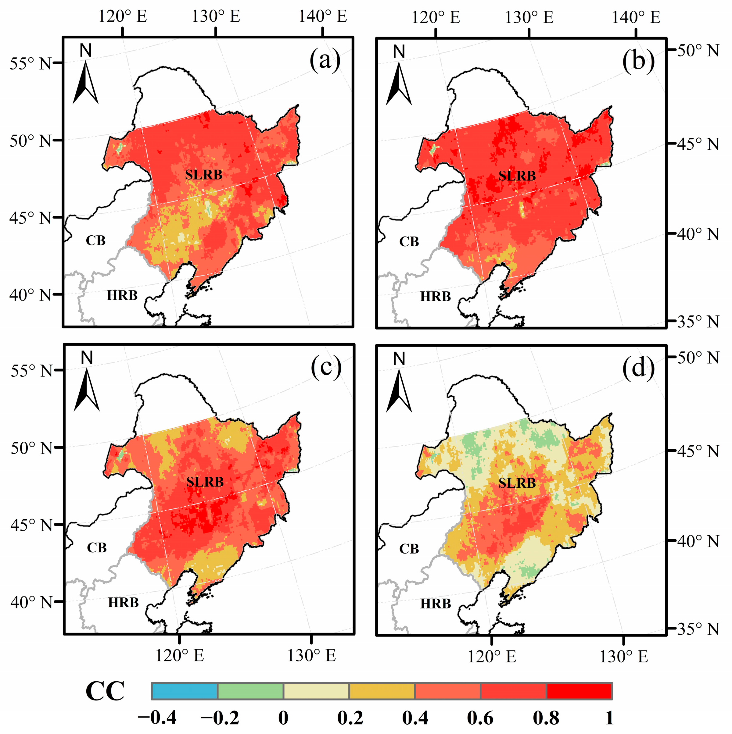
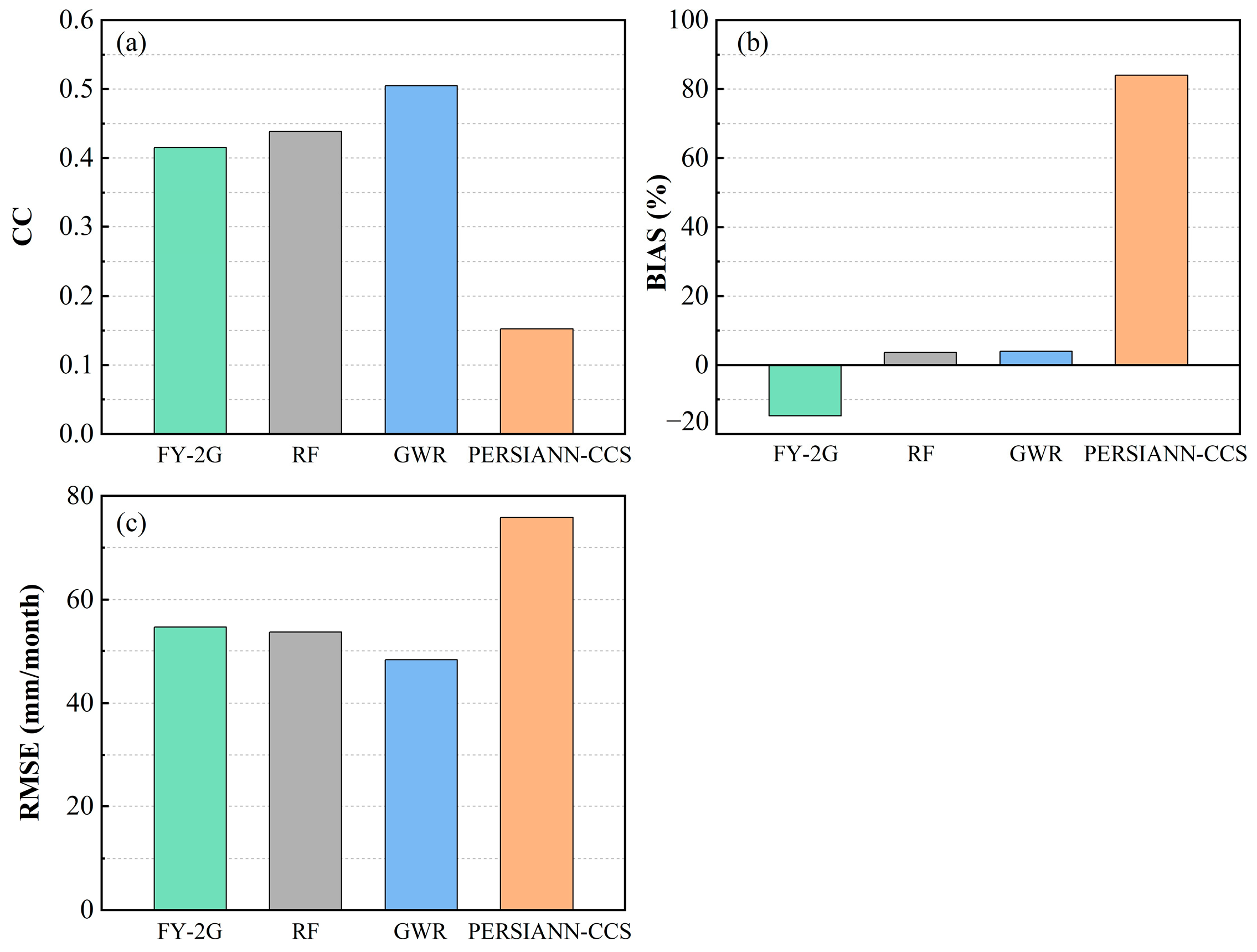
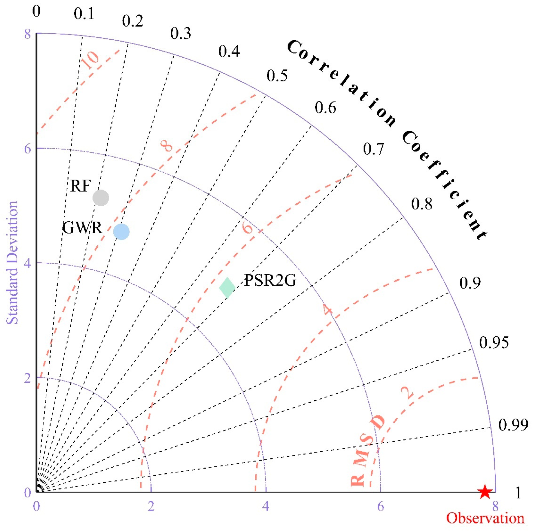
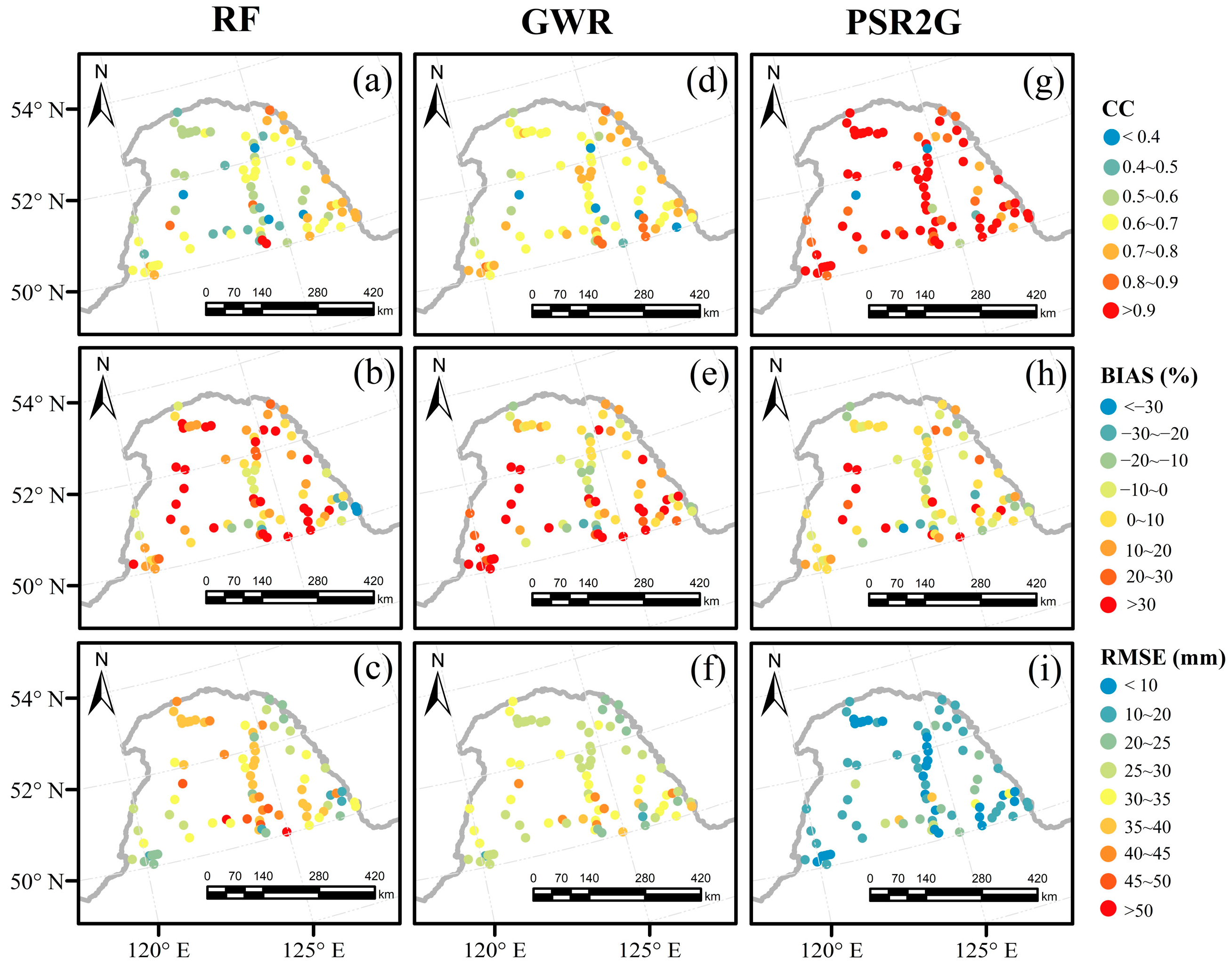
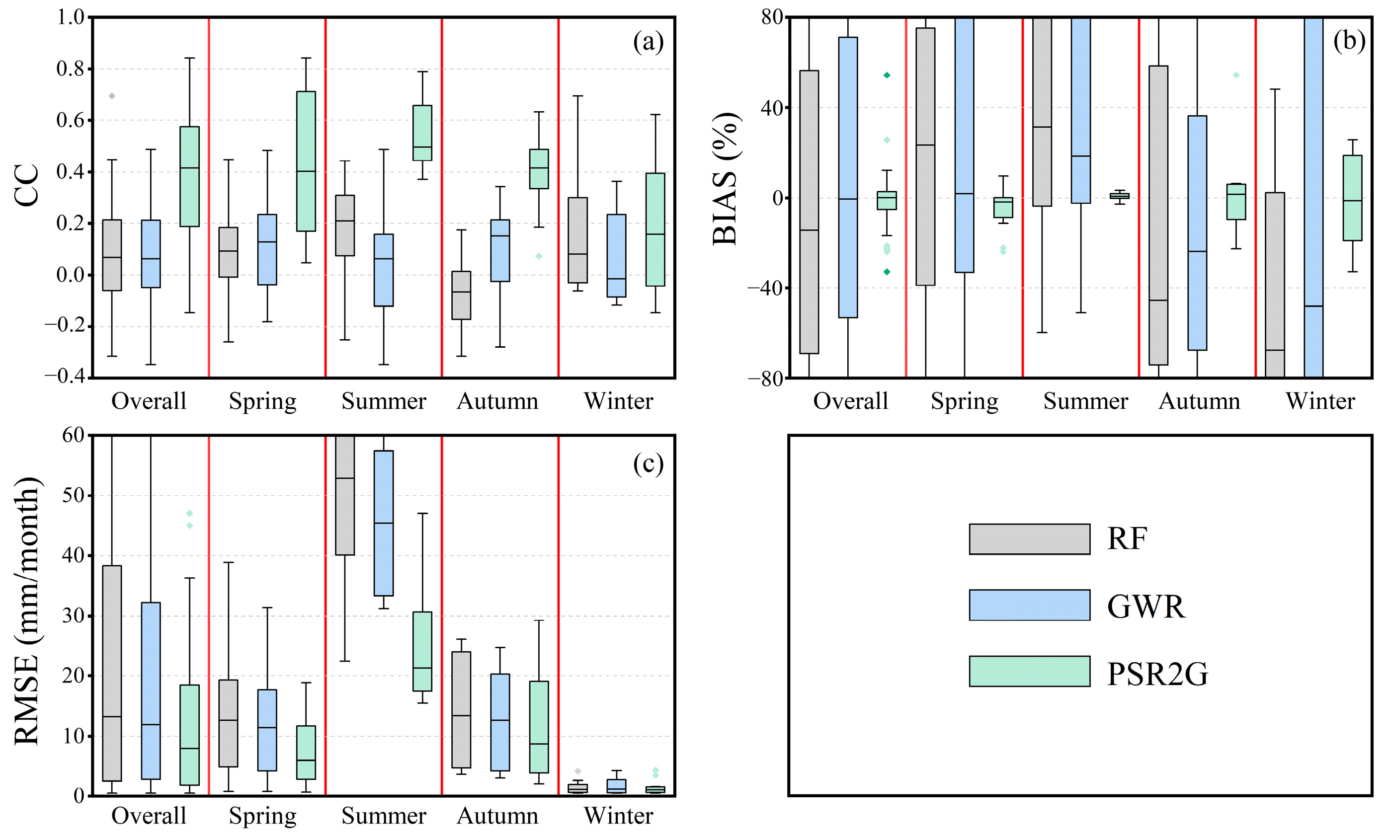
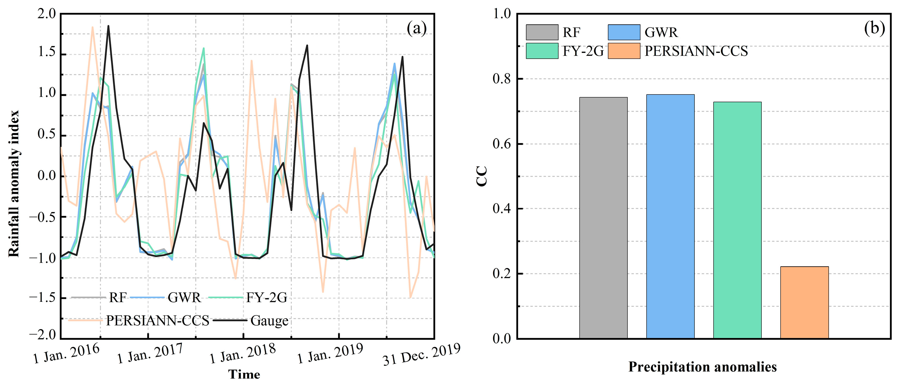
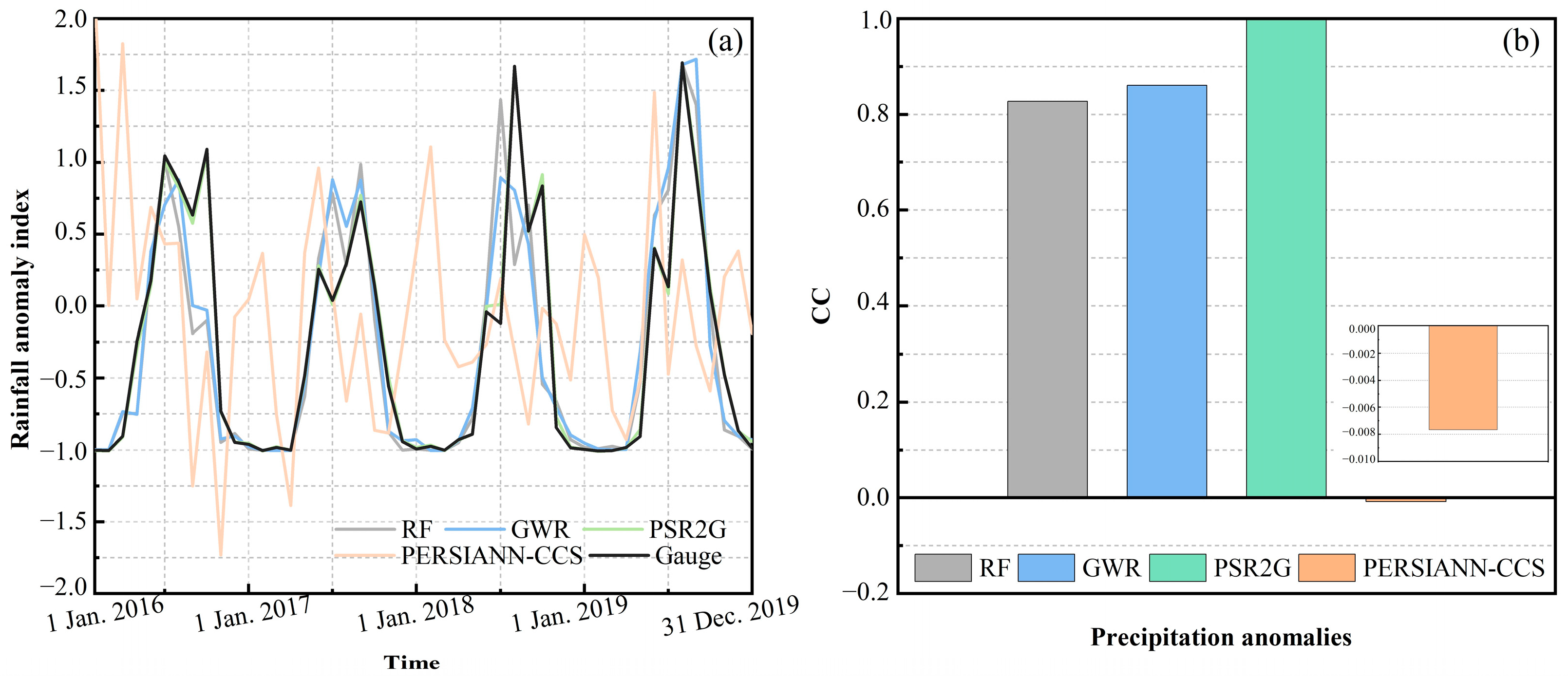

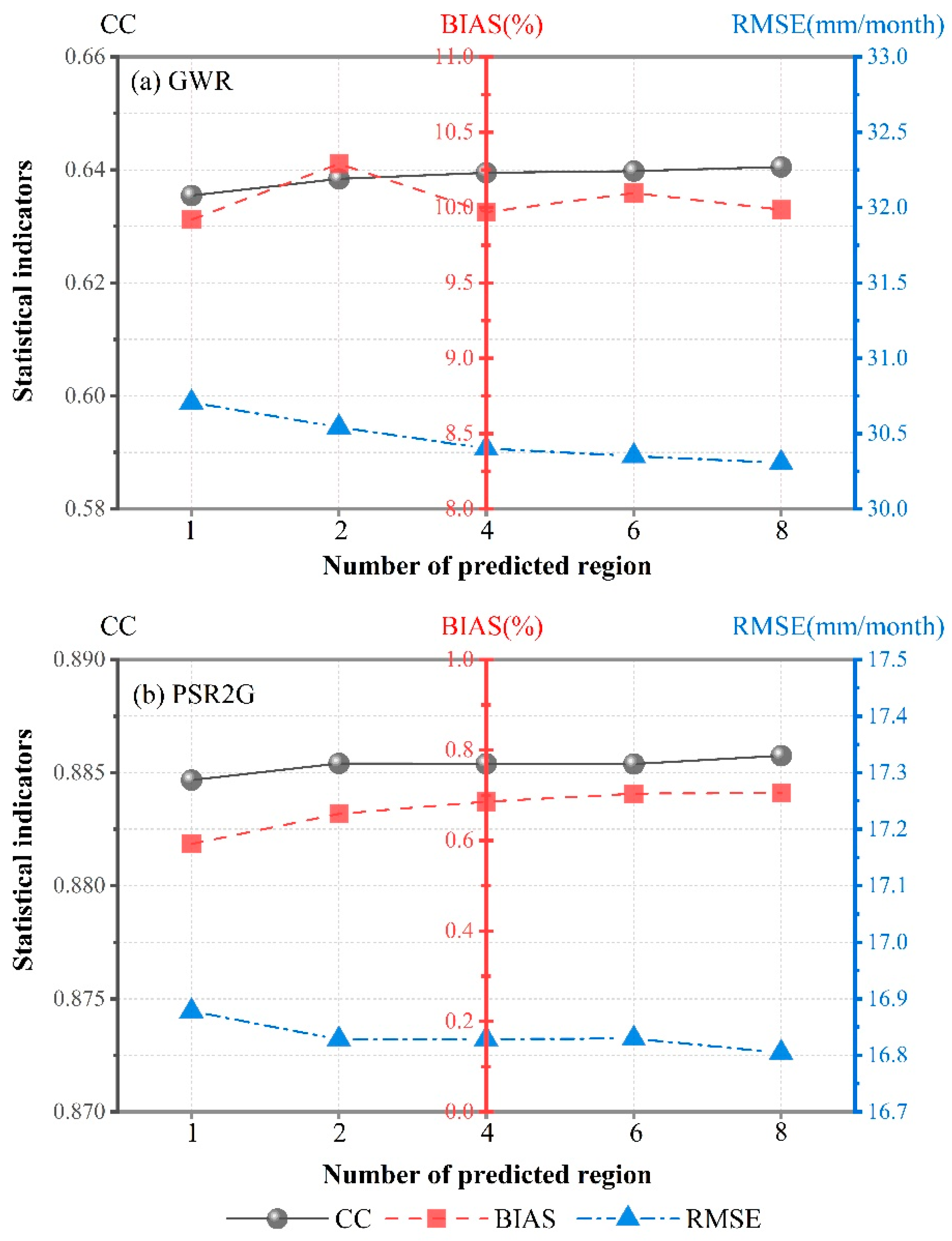
Disclaimer/Publisher’s Note: The statements, opinions and data contained in all publications are solely those of the individual author(s) and contributor(s) and not of MDPI and/or the editor(s). MDPI and/or the editor(s) disclaim responsibility for any injury to people or property resulting from any ideas, methods, instructions or products referred to in the content. |
© 2023 by the authors. Licensee MDPI, Basel, Switzerland. This article is an open access article distributed under the terms and conditions of the Creative Commons Attribution (CC BY) license (https://creativecommons.org/licenses/by/4.0/).