Article

Infrared Moving Small Target Detection Based on Space–Time Combination in Complex Scenes

1
State Key Laboratory of Laser Interaction with Matter, Changchun Institute of Optics, Fine Mechanics and Physics, Chinese Academy of Sciences, Changchun 130033, China
2
University of Chinese Academy of Sciences, Beijing 100049, China
*
Author to whom correspondence should be addressed.
Remote Sens. 2023, 15(22), 5380; https://doi.org/10.3390/rs15225380
Submission received: 27 September 2023 / Revised: 5 November 2023 / Accepted: 10 November 2023 / Published: 16 November 2023

Abstract

:
In the infrared small target images with complex backgrounds, there exist various interferences that share similar characteristics with the target (such as building edges). The accurate detection of small targets is crucial in applications involving infrared search and tracking. However, traditional detection methods based on small target feature detection in a single frame image may result in higher error rates due to insufficient features. Therefore, in this paper, we propose an infrared moving object detection method that integrates spatio-temporal information. To address the limitations of single-frame detection, we introduce a temporal sequence of images to suppress false alarms caused by single-frame detection through analyzing motion features within the sequence. Firstly, based on spatial feature detection, we propose a multi-scale layered contrast feature (MLCF) filtering for preliminary target extraction. Secondly, we utilize the spatio-temporal context (STC) as a feature to track the image sequence point by point, obtaining global motion features. Statistical characteristics are calculated to obtain motion vector data that correspond to abnormal motion, enabling the accurate localization of moving targets. Finally, by combining spatial and temporal features, we determine the precise positions of the targets. The effectiveness of our method is evaluated using a real infrared dataset. Through analysis of the experimental results, our approach demonstrates stronger background suppression capabilities and lower false alarm rates compared to other existing methods. Moreover, our detection rate is similar or even superior to these algorithms, providing further evidence of the efficacy of our algorithm.

Graphical Abstract

1. Introduction

Target detection is a crucial technology in the Infrared Search and Track (IRST) system [1]. It finds applications in various scenarios, such as guidance, early warning, and monitoring. However, practical challenges arise in target detection due to the small size of the targets or the long distance between the detector and the target. As a result, the proportion of pixels occupied by the target in the infrared image is often very small, typically less than 5 × 5 pixels. Moreover, the brightness of the target is relatively weak due to atmospheric scattering and absorption, making these targets difficult to detect directly. They are commonly referred to as infrared dim targets [2]. Infrared dim targets lack distinct shape, texture, and color information, further complicating their direct detection [3,4]. Additionally, natural environments introduce various complex backgrounds, such as clouds, trees, and buildings, which may appear within the detector’s field of view. These backgrounds often have higher brightness than the target and contain more complex edge clutter information [5]. Furthermore, device manufacturing defects and random electrical noise during system operation can introduce high-brightness point noise into the original image [6]. All these factors pose challenges to accurate target detection, particularly in complex scenes involving small objects.
The detection of dim and small targets can be broadly classified into single-frame-based detection and sequence-based detection. Early common methods for detecting targets in single-frame images include median filtering [7], max-mean/max-median filter [8], bilateral filter [9], the Two-Dimensional Least Mean Square (TDLMS) algorithm [10], frequency domain transformation [11,12], and the top-hat algorithm based on morphological transformation [13], among others. In addition, certain methods that leverage sparsity and low rank have demonstrated notable outcomes. A noteworthy algorithm in this domain is Robust Principal Component Analysis (RPCA) [14], which exhibits superior noise-resistance capabilities compared to traditional Principal Component Analysis (PCA). For instance, Fan Junliang et al. [15] initially employed Butterworth high-pass filtering to preprocess the original image, effectively eliminating background interference. Subsequently, RPCA was applied to decompose the filtered outcome, facilitating the identification of dim and small targets amidst the sparse foreground. It is important to acknowledge that in scenarios where the image background is relatively complex, certain evident background edges and corners also display varying degrees of sparsity. This circumstance can lead to inadvertent decomposition into sparse matrices, subsequently affecting the subsequent target detection process. To mitigate this challenge, Gao et al. [16] proposed the image block matrix method (IPI), wherein the reconstructed image block matrix generally manifests improved low-rank performance compared to the original image. The research community recognized and further refined this concept concerning the decomposition of background edge errors [17,18]. However, it should be noted that related models still face limitations in practical applications due to their dependency on manual parameter selection and inadequate generalization performance. To address this issue, Li et al. [19] introduced the LRR-NET model, which effectively integrates the LRR model with deep learning techniques. By transforming the regularization parameters into trainable parameters within the deep neural network architecture, the reliance on manual parameter tuning is substantially reduced.
Models based on human vision (HVS) have a significant impact on improving the accuracy of detecting small and weak infrared targets in complex scenes while reducing false alarm rates [20]. The core concept of these models is to utilize local contrast, which refers to the grayscale difference between the current location and its local neighborhood. In practical applications, scholars employ various parameter values and calculation methods for local contrast based on specific problem requirements, with some algorithms also considering the suppression of background edges and noise. In terms of local contrast types, one approach involves measuring the grayscale difference between multiple pixels within the central region and several pixels in the surrounding neighborhood. This information enables the effective suppression of high-brightness, evenly distributed background areas, making the target easier to detect. Classical filters used in this context include the LoG (Laplacian of Gaussian) filter convolutional kernel [21] and the DoG (Difference of Gaussian) filter [22]. To improve the performance of the DoG filter, Han et al. [23] replaced the circular Gaussian kernel function with an elliptical Gabor kernel function based on the directional differences between the real target and background edges. By adjusting the major axis angle of the ellipse, the filter demonstrates directional discrimination ability and better suppresses background edges. Another approach, known as ratio-type local contrast, enhances the central pixel by leveraging the grayscale ratio of multiple pixels in the central region and the surrounding circular neighborhood, thereby acting as an enhancement factor. Classic algorithms employing this approach include LCM (Local Contrast Measure) [24], ILCM (Improved LCM) [25], which introduces the average number of sub-blocks as parameters to suppress highlighting noise, and NLCM (Novel LCM) [26], which retains the noise suppression capability of ILCM and effectively addresses the smoothing of small targets. For small targets without distinctive features, the contrast gap between them and the surrounding background can be the most effective spatial characteristic. However, in complex backgrounds, non-target regions with relatively high contrast may appear due to the chaotic distribution of grayscale values. As a result, algorithms solely relying on contrast also respond to these areas, leading to the inaccurate extraction of the true target.
With the advancement of deep learning, scholars have explored the use of neural networks to extract deep features from small targets. Wu et al. [27] proposed the UIU-NET framework for multilevel and multiscale representation learning of objects. Zhou et al. [28] introduced a feature extraction module based on dual pooling, combining average pooling and maximum pooling, to mitigate sidelobe effects and the influence of blurry contours in remote sensing images, thereby enhancing target information. The ORSIm detector, proposed by Wu et al. [29], aims to incorporate both rotational-invariant channel features constructed in the frequency domain and original spatial channel features. They employ a learning-based strategy to refine the spatial-frequency channel feature (SFCF) and obtain advanced or semantically meaningful characteristics. Deep neural networks excel in extracting target features and effectively distinguishing targets from background noise. However, weak and small targets offer limited spatial features, while certain prominent structures, such as buildings, trees, and clouds in complex scenes, share similar spatial characteristics with small targets. Consequently, algorithms that primarily rely on extracting spatial features may mistakenly identify these backgrounds as targets, resulting in a higher false alarm rate. To address these challenges, the incorporation of temporal features is crucial in distinguishing whether images with target features truly represent moving targets.
Sequence-based detection is commonly used to distinguish the foreground (moving object) and the background (relatively still object) of an image by analyzing the object’s motion. There are three common motion detection methods: the interframe difference method [30], the background modeling method, and the optical flow method. Among them, the inter-frame difference method can only detect the edge contour of the moving object, leaving many holes in the interior. It becomes ineffective when background changes occur between frames. Background subtraction involves three steps, background modeling, foreground extraction, and foreground detection, with the most crucial step being background modeling. Common background modeling methods include Gaussian mixture model (GMM) [31], Codebook background modeling method [32], and Visual Background Extractor (ViBe) [33] algorithms. However, background modeling-based methods often exhibit “ghosting” phenomena due to the movement of the target. Additionally, both methods fail when there are background changes, such as camera movement or scene lighting adjustments. The optical flow method [34,35] is capable of calculating a global optical flow field. However, when applied to small infrared target images with complex backgrounds without preprocessing, pixel-based optical flow calculations are also disturbed by background changes, resulting in a disordered optical flow that hinders small target detection.
Currently, researchers predominantly utilize methods based on single-frame or sequence images for infrared small target detection. By analyzing the limited information of the target imaging properties and spatial information in a single frame image, researchers construct a model to enhance the target and suppress the background [36]. However, single-frame detection methods encounter challenges of high false alarms due to specks with similar spatial information and background interference. To address this, this paper introduces multi-frame sequence information into single frame image detection. By detecting the motion characteristics of the target in the sequence, it aims to reduce false alarms in single frame detection and enhance detectable targets. The main contributions of this paper include:
  • Proposing an image-preprocessing method that leverages the local saliency of images for object enhancement.
  • Proposing a multi-scale layered contrast feature extraction method that effectively suppresses false positives caused by local grayscale fluctuations in pixels.
  • Utilizing a spatiotemporal context to globally “track” the image, obtaining motion information for each pixel, and using statistical characteristics to separate information related to moving targets, thereby generating an abnormal motion feature map of the image.
  • Employing motion features to perform non-target suppression and target enhancement on suspicious target detection results obtained from the multi-scale layered contrast feature extraction method, ultimately determining target positions through threshold segmentation.
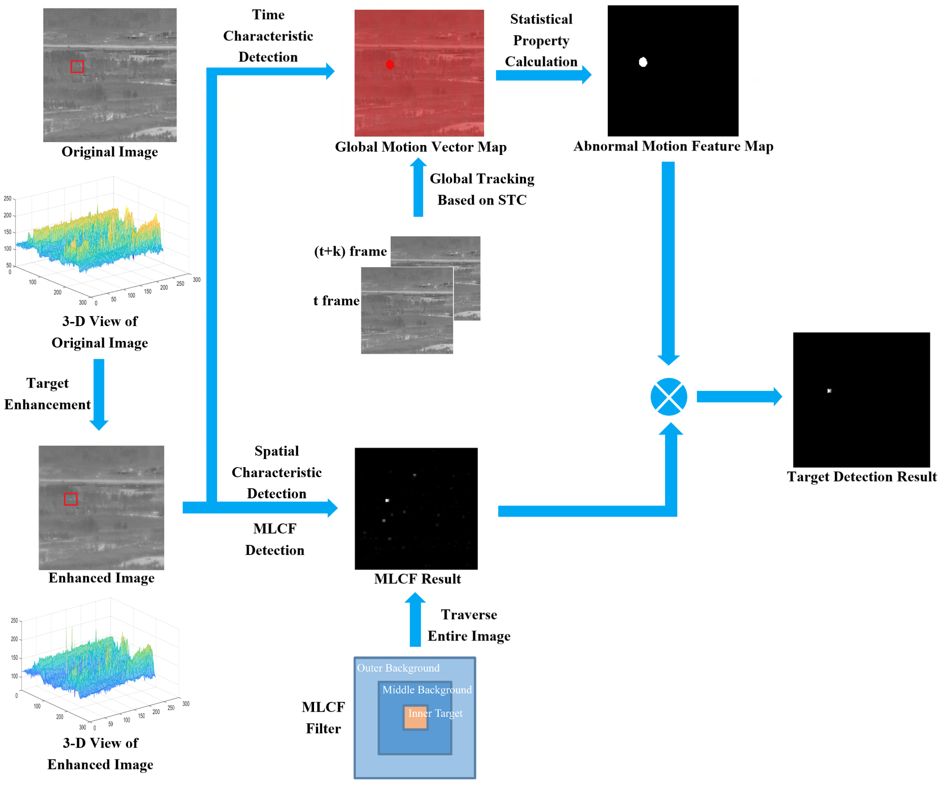
2. Proposed Method

A flowchart illustrating the proposed method is presented in Figure 1. The method mainly comprises the following components: first, the local saliency of the image is utilized for target enhancement; second, the layered contrast feature is employed to detect potential targets; subsequently, the spatio-temporal context is utilized to acquire the motion features of all image pixels, enabling the detection of actual moving targets and the suppression of false alarms; finally, the target location is determined through threshold segmentation.

2.1. Target Enhancement and Filtering

Infrared small target images often suffer from challenges such as small target size and low contrast, which poses difficulties in target detection. Hence, it is necessary to perform target enhancement preprocessing. One common approach for target enhancement is corner detection, which can be achieved through methods such as DoG filtering, LoG filtering, and others. These methods are capable of extracting image details. However, in scenarios with more complex background interference, they may not effectively enhance the target and could inadvertently suppress the background as illustrated in Figure 2. In our method, we aim to reduce false alarms and enhance target detection accuracy by calculating abnormal motion in the image sequence to determine the target’s position. Consequently, preserving the background with distinct features becomes crucial. Considering these requirements, this paper proposes a filtering method that adjusts the local variance of the image based on its local significance.
Firstly, we calculate the local significance of the image based on the region gray level difference:
S ( I ( x , y ) ) = ( x , y ) ( x , y ) W ( I ( x , y ) ) D c ( I ( x , y ) , I ( x , y ) )
where D c ( I ( x , y ) , I ( x , y ) ) is the absolute difference between the grayscale of two pixels, and W ( I ( x , y ) ) is the inverse distance weight.
The resulting local significance graph is shown in Figure 3, and we can see that it preserves the outlier and the target very well.
Next, we calculate the local standard deviation of the original image. If the significance here is relatively low, we should compress the pixel grayscale value distribution here.
Take the collection of local pixels centered on I ( x , y ) as I = { I 1 , I 2 , , I n } , then define:
I ˜ = I m e a n ( I ) = I 1 ˜ , I 2 ˜ , , I n ˜
s t d ( I ( x , y ) ) = i = 1 n I i ˜ 2 n 1
The transformed pixel gray value is defined as I′, and has:
I ˜ = I m e a n ( I ) = I 1 ˜ , I 2 ˜ , , I n ˜
I ˜ = α I ˜
s t d ( I ( x , y ) ) = i = 1 n I i ˜ 2 n 1 = S ( I ( x , y ) )
α i = 1 n I i ˜ 2 n 1 = S ( I ( x , y ) ) = α · s t d ( I ( x , y ) )
α = S ( I ( x , y ) ) s t d ( I ( x , y ) ) , s t d ( I ( x , y ) ) 0 0 , s t d ( I ( x , y ) ) = 0
I m e a n ( I ) = α · ( I m e a n ( I ) )
I = α · ( I m e a n ( I ) ) + m e a n ( I )
The transformed image is shown in Figure 4. As can be seen from the 3D view plot, we succeeded in enhancing the target without affecting the background features. The signal-to-clutter ratio (SCR) in Figure 4 is calculated to be significantly improved:
S C R i n = 0.5593 S C R o u t = 2.5374

2.2. Calculation of MLCF

Based on the Human Visual System (HVS), the grayscale value of a target in an infrared image is typically higher than the grayscale value of its surrounding background pixels [37]. However, in complex scenes, there may be a phenomenon called “gray diffusion”, where there are image blocks with high brightness in the center pixels and a gradually decreasing brightness in the surrounding pixels. Simply using the grayscale difference between the center and surrounding areas for calculation can result in false alarms after binarization, as it may also detect edge corners, background disturbances, and areas with small grayscale fluctuations that exhibit this “gray diffusion” phenomenon, such as small buildings or small gathered clouds. Figure 5 shows the result of LCM processing, where areas that are not actual targets are enhanced. To address this, we propose a layered contrast model inspired by Wu et al. [38]. This model has a three-layer structure: the target with a higher grayscale value is situated in the inner region, while the background with a lower grayscale value is located in the outer and middle regions (see Figure 6). By calculating pixel by pixel throughout the entire image using this layered model, we can obtain more comprehensive contrast information for target–background separation, complete target extraction, and background suppression. The layered model allows us to obtain more target contrast features to highlight the target and suppress the background. The original model utilized average value calculation within block areas. However, due to the lack of a specific rule in the distribution of image pixels, forced block calculation would separate parts of the background with higher gray values and average them with the low gray values in their respective subregions. This results in lower grayscale values in the sub-blocks, leading to distortion of the neighborhood gradients and detection errors as depicted in Figure 7. Additionally, small targets with very small sizes could have their gray levels reduced due to the averaged calculation within subregions, making their detection challenging. Therefore, the proposed approach in this paper eliminates the use of subregions between the layers and retains only the layered regions. After implementing target enhancement as described in Section 2.1, Gaussian filtering is applied to the target to both smooth the image and reduce the degree of reduction in target brightness.
Compared with some background interference, the target usually has strong independence, and there is a clearer and more neat gray change between the target and the background. Therefore, we add a step to calculate the gray change degree between each layer of the three-layer model:
G ( I M ) = max { max ( i n n e r ) max ( m i d d l e ) , 0 }
G ( M O ) = max { max ( m i d d l e ) max ( o u t e r ) , 0 }
L C F = max { G ( I M ) · ( G ( I M ) G ( M O ) ) , 0 }
where the function max ( · ) applies morphological operations on the image using a structural element based on the parameters specified within the parentheses. The structural element, as illustrated in Figure 6a, has a value of 1 assigned to the layers inside the parentheses, while the remaining layers have a value of 0. The function max { · } retrieves the maximum value from the results enclosed within the curly braces.
Change the size of the layered model to obtain LCF at different scales:
M L C F = max { L C F s z 1 , L C F s z 2 , L C F , }

2.3. Calculate Abnormal Motion

2.3.1. Spatio-Temporal Context

Tracking key points in an image is a common approach used to calculate the motion feature map of the image. This can be achieved through popular tracking methods, such as the interframe difference method and background modeling method. However, these methods can become less effective and fail to accurately detect real moving targets when the detector is not static or when there is background motion due to specific requirements or unforeseen interference. The optical flow rule, which is typically used to track pixel movement based on slight changes in each pixel in sequence images provided by infrared imaging, can significantly impact the accuracy of the optical flow calculation. For dim and small targets, the minuscule errors in pixel calculations can also result in detection failures.
In this paper, point-by-point tracking is accomplished using the spatio-temporal context (STC) method [39]. The premise of this method requires the movement of the target between two frames to be within the suitable distance for the algorithm. Instead of relying on the optical flow method, we utilize the spatial context as the feature for tracking the target pixel. Although the gray value of the pixel may slightly fluctuate within the sequence, its overall feature as an image block remains relatively stable. To accurately detect the target and calculate abnormal motion relative to the entire image, sufficient data are required. Therefore, instead of calculating key points, we choose to perform calculations on global pixels. The graphical model illustrating this method is depicted in Figure 8. In this model, x represents the target location within the context, and o represents the actual location of existing objects in the scene. By maximizing the confidence map M ( x ) , we can achieve the accurate tracking of the target pixels. The confidence map estimates the likelihood of the object position:
c ( x ) = P ( x | o )
In the present frame, we have the object position x * (i.e., the coordinates of the center of the object being tracked). The venter solicitation is defined as X c = { c ( z ) = ( I ( z ) , z ) | z Ω c ( x * ) } , where I ( z ) represents the image intensity at position z , Ω c ( x * ) is the neighborhood of the position. By marginalizing joint probabilities P ( x , c ( z ) | o ) , the object position likelihood function can be calculated by the following formula:
c ( x ) = P ( x | o ) = c ( z ) X c P ( x , c ( z ) | o ) = c ( z ) X c P ( x | c ( z ) , o ) P ( c ( z ) | o )
where the conditional probability function P ( x | c ( z ) , o ) defined as:
P ( x | c ( z ) , o ) = h s z ( x z )
Context prior probability P ( c ( z ) | o ) defined as:
P ( c ( z ) | o ) = I ( z ) ω σ ( z x * )
where I(·) is the image intensity that represents the appearance of the context, and ω σ ( · ) is the weighting function defined by:
ω σ ( z ) = a e | z | 2 σ 2
where a is a normalization constant that restricts P ( c ( z ) | o ) to the range from 0 to 1 that satisfies the definition of probability and σ is the scale parameter.
The confidence graph for the location of the object is modeled as:
c ( x ) = P ( x | o ) = b e | x x * α | β
where b is the normalized constant, α is the scale parameter, and β is the shape parameter. Refer to Figure 9 for different values of parameters β .

2.3.2. Filtering Motion Based on Statistical Features

With x as the center, we obtain the context regions patch1 and patch2 with size s z corresponding to x . These patches are extracted from the two frames of images in the sequence. The next step is to calculate the confidence map of patch2, which can be expressed as follows:
F ( c ( x ) ) = F ( h s z p a t c h 1 ( x ) ω σ ( x x * ) )
h s z = F 1 ( F c ( x ) F ( p a t c h 1 ( x ) ω σ ( x x * ) ) )
c m a p ( x ) = F 1 ( F ( h s z p a t c h 2 ( x ) ω σ ( x x * ) ) )
Take the coordinates where the maximum value of c m a p ( x ) is ( x r , y r ) , then obtain the displacement vector object x :
r = r ( x ) = ( x r , y r ) ( s z 2 , s z 2 )
After all the motion features are calculated for the whole image, the modal filtering is carried out to remove the noise, and the results are shown in Figure 10.
As illustrated in Figure 10, the presence of context has an impact on the motion vectors of pixels. Pixels with high significance tend to exhibit similar motion vectors in their surroundings, while different motion vectors exhibit aggregation.
In a global sports field setting, most of the background tends to have the same motion vector, which represents the global motion. However, the target object will exhibit different motion compared to the background. By leveraging the statistical characteristics of the target’s motion, we can identify pixels that belong to abnormal or distinct motion patterns.
Firstly, we need to define the global displacement vector set as:
R = r 1 , r 2 , r 3 , , r k , , r K
and the set of coordinates of each vector as:
S Z r K = ( x 1 k , y 1 k ) , ( x 2 k , y 2 k ) , , ( x n k , y n k )
In addition, the abnormal motion vectors belonging to the target should have convergence. The variance of each coordinate set is calculated as the degree of polymerization of the vectors:
D o P k = 1 λ + s t d ( X k · Y k )
where X k = x 1 k , x 2 k , , x n k , Y k = y 1 k , y 2 k , , y n k .
The DoP (Degree of Possibility) value is utilized to represent the probability that a point with a specific motion vector belongs to the target pixel and its vicinity, denoted as ω k . The value of n k corresponds to the number of points in the entire image having the same motion vector k. Based on prior knowledge, certain criteria are set for distinguishing motion errors and background regions. If the number of points with the same motion vector is less than a threshold value T l i m 1 , they are considered motion detection errors and assigned a probability of 0. Conversely, if the number is larger than a certain threshold value T l i m 2 , they are deemed part of the background and also assigned a probability of 0. In addition, individual anomalies are observed in our data where certain spots move with the camera, resulting in their movement relative to the background while retaining their coordinates in the image. When a spot holds higher significance in the image region, the calculated displacement change of the spot and its surrounding pixels in motion detection is (0, 0). In comparison, the target exhibits small displacement between frames, both relative to the background and within the image. Due to the small scale of the target, even the slight displacement of a few pixels can be detected. Thus, the ω k value of a point with a motion vector of (0, 0) is directly defined as 0. In summary, the weights ( ω k ) calculated based on the motion features can be defined as follows:
ω k = 0 , r k = ( 0 , 0 ) 0 , n k < T l i m 1 | | n k > T l i m 2 D o P k , T l i m 1 n k T l i m 2
where r k refers to the motion vector k, n k represents the number of pixels in the image associated with the motion vector r k , T l i m 1 and T l i m 2 are threshold values used for filtering the number of vectors, and D o P k represents the probability of the motion vector k belonging to the target pixel and its vicinity, which is calculated using Formula (28).
Assign ω k to all vector coordinates as weights to obtain abnormal motion feature maps (AMF) as shown in Figure 11.

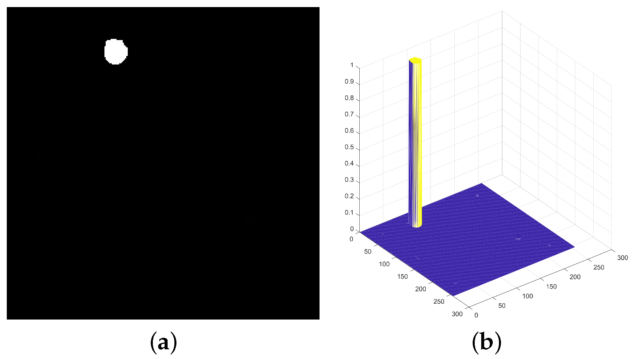
2.3.3. Calculation of Target Feature Map

By combining the grayscale contrast information of a single-frame image in the spatial domain and the motion feature information of a sequence image in the temporal domain, we can form the final target feature map T:
T = M L C F · ( A M F + λ )
where λ is the regular term.
Finally, calculate the adaptive threshold for binarization to obtain the position of the target as shown below:
m = M L C F · m + v v a r
where m is the mean of the target feature map, v a r is the variance of the target feature map, and v is an adjustable parameter used to determine the weighting of differences in threshold segmentation.

3. Experimental Results and Analysis

We prepared six infrared image sequences for conducting algorithm evaluation experiments. Each sequence consists of images with a size of 256 × 256 pixels. Figure 12 displays the six different datasets [40]. The data acquisition scenarios encompass various sky backgrounds and ground backgrounds, including complex buildings and trees. Detailed information about each of the six sequences is provided in Table 1. Simulation and demonstration are based on Intel(R) Core(TM) i5-10200H, NVIDIA GeForce GTX1650Ti.

3.1. Ablation Experiments

The algorithm consists of three modules: image preprocessing, spatial feature extraction, and motion feature extraction. The image enhancement module enhances isolated pixels while preserving background features. The spatial feature extraction module extracts initial targets based on spatial characteristics and forms the fundamental basis of the algorithm. The motion feature module filters the extracted candidate “targets” from the previous module based on their motion characteristics in the temporal sequence. During this stage, genuine targets are preserved while suppressing noise or background interference that is unrelated to the targets, thereby effectively suppressing false alarms. Ablation experiments are conducted on the complete dataset to assess the effectiveness of the preprocessing module and the motion feature extraction module. The control groups consist of four algorithm flows: the complete algorithm flow (Ours), the algorithm flow without the image preprocessing module (No ImgPre), the algorithm flow without the motion feature extraction module (No MoFeature), and the algorithm flow with only the spatial feature extraction module (MLCF).
The detection performance of the algorithm is evaluated using Receiver Operating Characteristic (ROC) curves, as shown in Figure 12, from the ablation experiments conducted on various datasets. Along the horizontal axis, the false alarm rate is depicted, while the vertical axis represents the detection rate. A larger area under the curve signifies improved detection performance of the algorithm.
Overall, the motion feature extraction module demonstrates a substantial capability to suppress false alarms as concluded from the analysis conducted above. Furthermore, the presence of the motion feature extraction module enhances the detection capability, especially in scenes with complex background interference, exemplified by datasets 3, 4, and 5 (shown in Figure 13). By enhancing the contrast of isolated pixels, the image preprocessing module directly improves the detection performance of MLCF, thereby enhancing the overall effectiveness of the algorithm. In images with minimal background interference and prominent targets, such as in datasets 1 and 6 (as depicted in Figure 13), the preprocessing module inadvertently enhances pixels with slight grayscale differences that lie beyond the designated targets. A comparison between two specific experimental groups in this dataset (MLCF and No MoFeature) indicates that the absence of the motion detection module’s false alarm suppression capability leads to a higher incidence of false alarms in the detection results. For practical applications, algorithm optimization needs to consider the specific characteristics of the dataset.

3.2. Algorithm Performance Evaluation

Compare our approach to the following six foundational algorithms, including NWTH, MPCM, FMM, SR, ViBe, and IPI. NWTH [41] is a morphological-based algorithm that utilizes a ring-shaped structuring element, distinguishing it from the conventional top-hat algorithm. The outer and inner dimensions of the structuring element are denoted as R o and R i , respectively, and should be appropriately adjusted to match the size of the target. Both MPCM [42] and FMM [5] are contrast-based object detection algorithms. The size of the sliding window is a critical parameter for these algorithms and should be adjusted to match the target’s size. SR [43] utilizes Fourier Transform to obtain the magnitude spectrum and phase spectrum of an image. The algorithm applies linear spatial filtering, such as a 3 × 3 mean filter, to the magnitude spectrum. It then subtracts the filtered magnitude spectrum from the original magnitude spectrum to generate a residual spectrum. After performing the inverse Fourier Transform on the residual spectrum, a saliency map is obtained. The size of the filtering kernel is an adjustable parameter in this process. The ViBe algorithm [44] is based on establishing a background model and identifying foreground objects by detecting pixels in the current frame that significantly deviate from the background model. The algorithm compares each pixel’s value with that of the background pixels and applies a threshold to classify each pixel as the foreground or background. Parameters are utilized to model the background and determine the threshold. The IPI [16] algorithm segments an image into smaller patches and reassembles them to generate a reconstructed image with a lower rank than the original image. The size of the patch images and the sliding step of the window directly influence the rank of the reconstructed image, thereby impacting the overall detection performance of the algorithm. The selected parameters in this paper are well suited for our dataset. All parameters of these methods are optimally set according to established references, and the specific parameter settings are shown in Table 2.
The background suppression results of different methods, including two-dimensional (2D) images and three-dimensional (3D) images, are shown in Figure 13. Then, we subjectively and objectively evaluate their performance in Section 3.2.1 and Section 3.2.2.

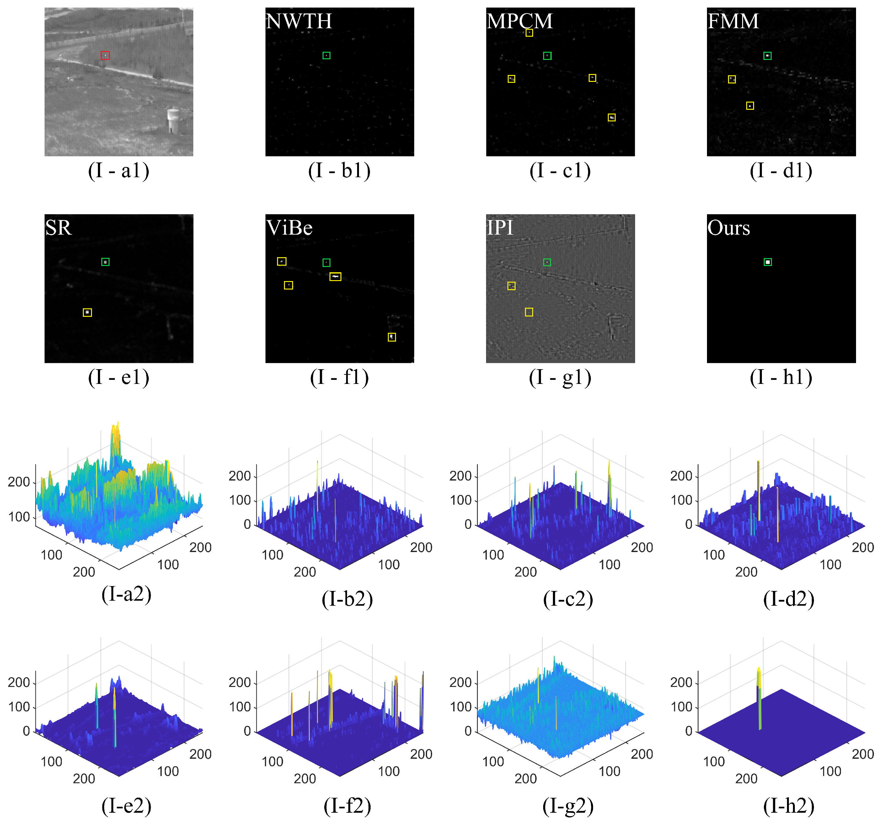
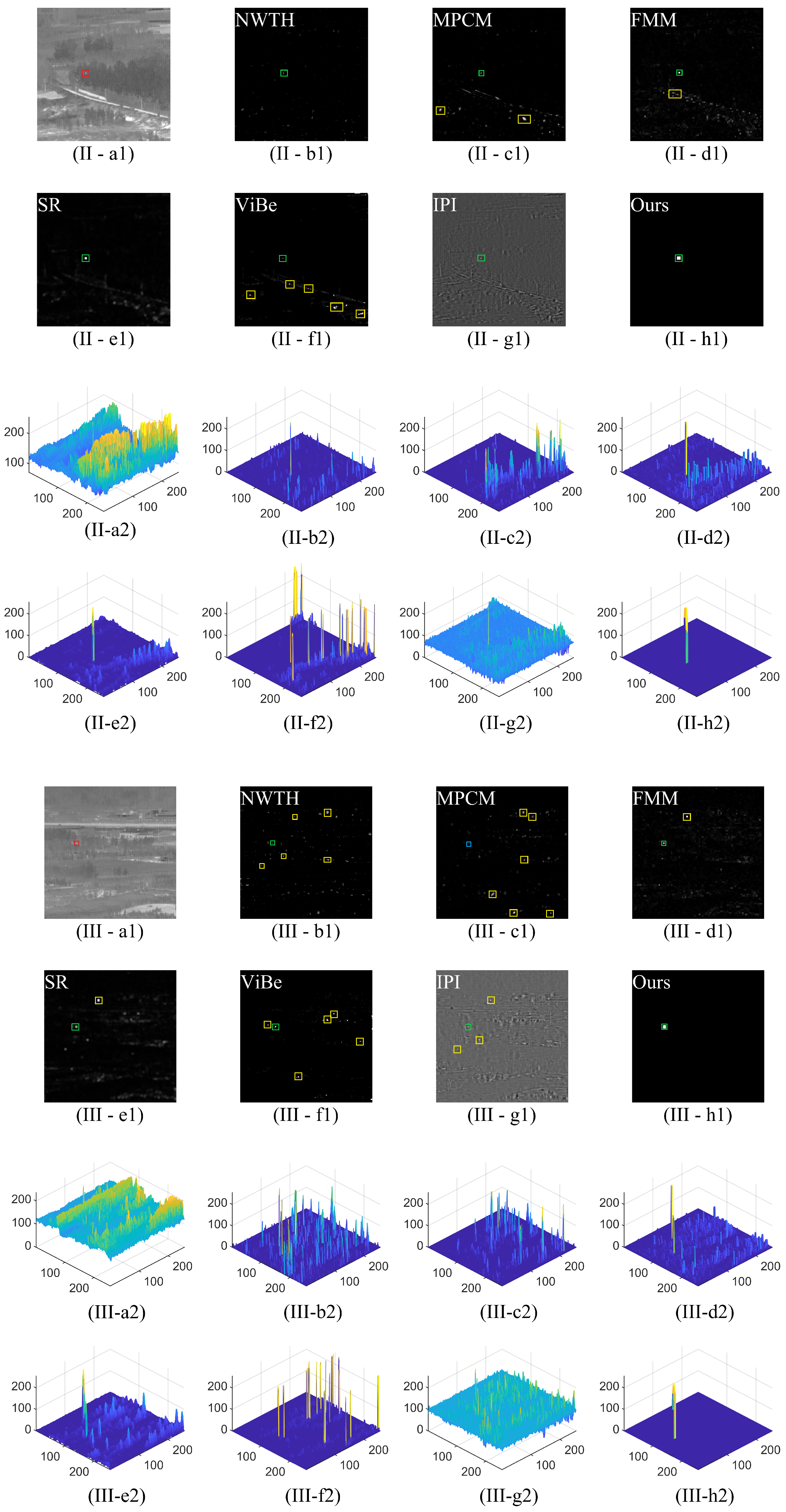
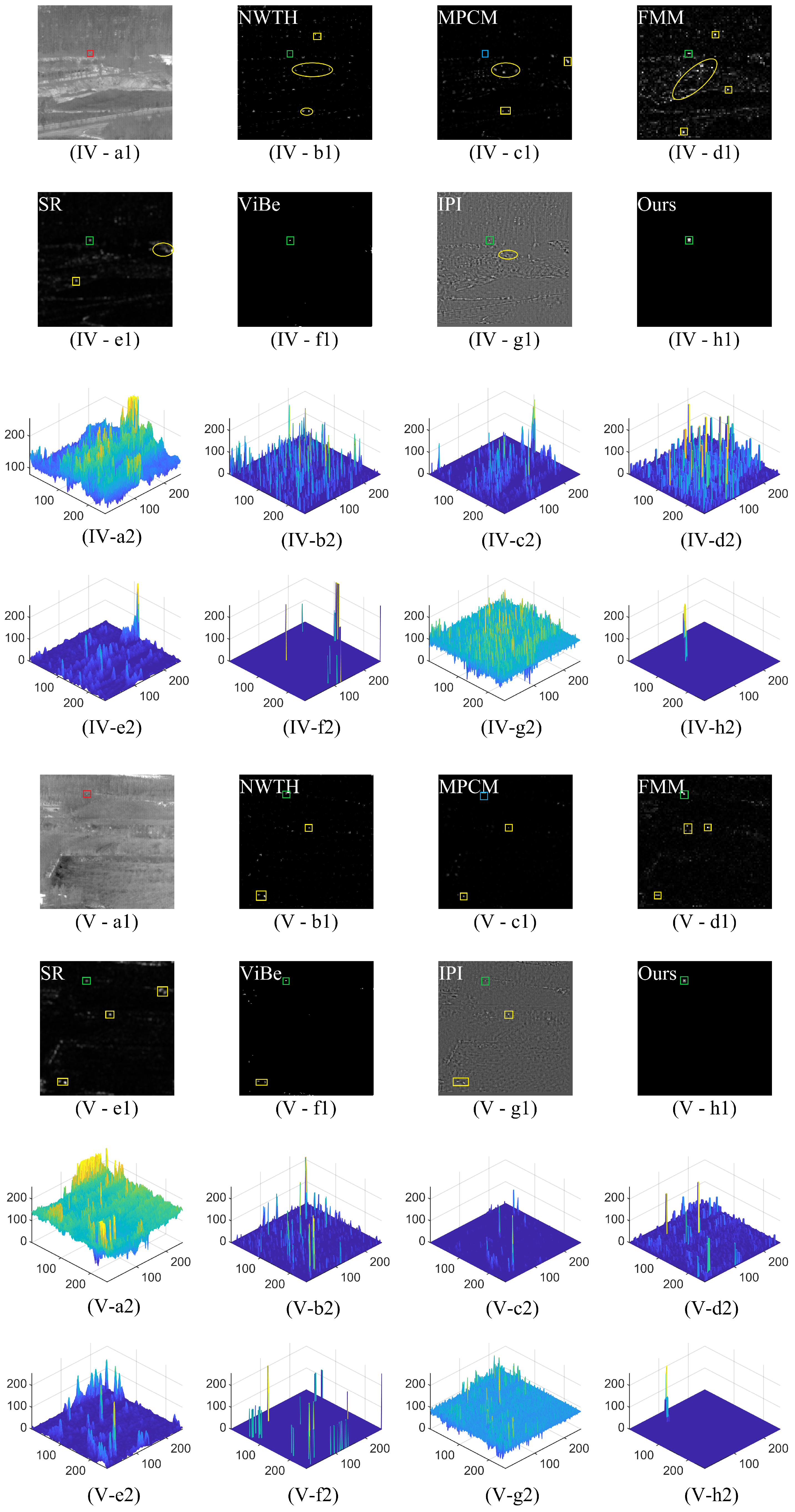
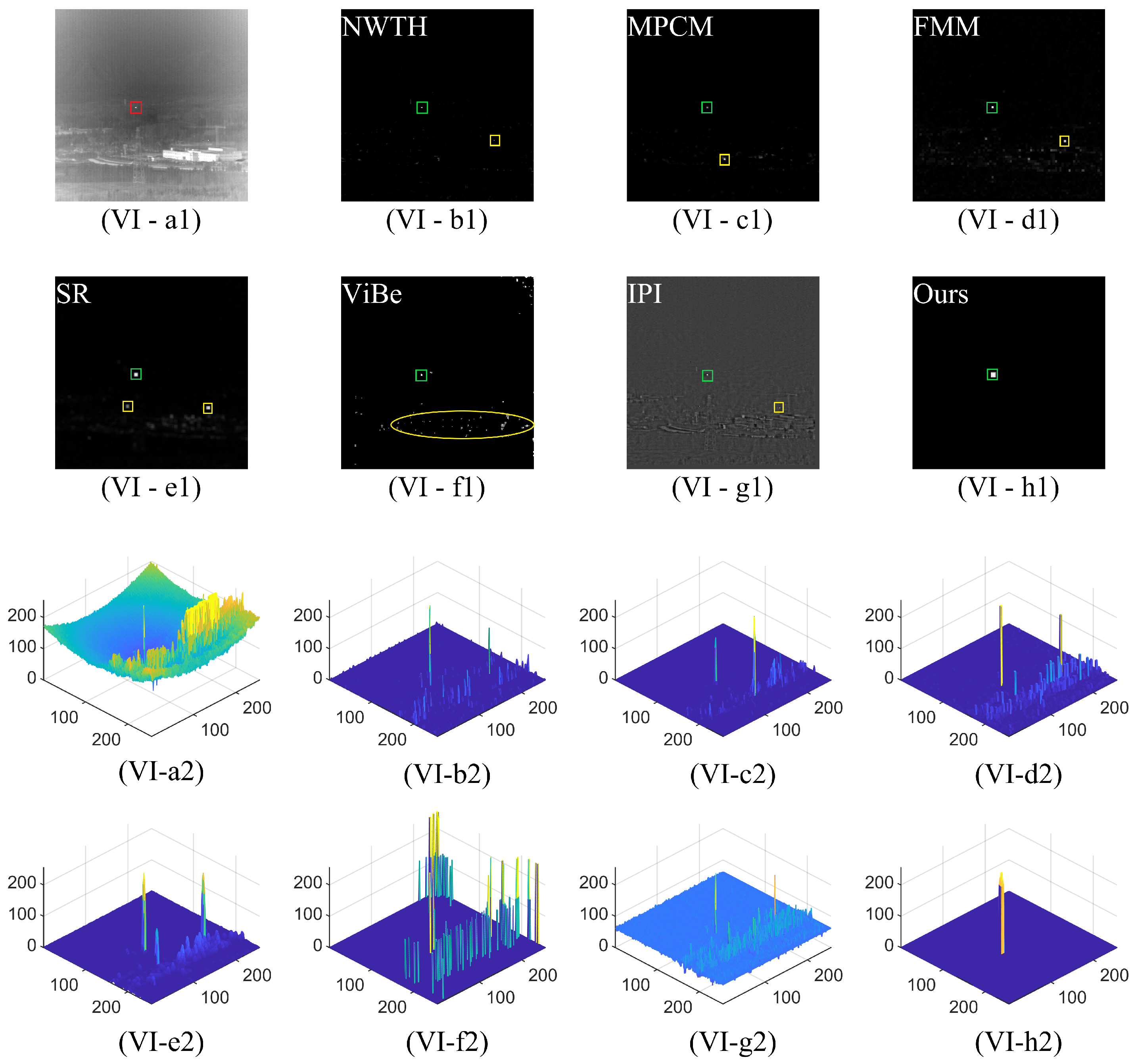
3.2.1. Subjective Evaluation

By observing the results of background suppression in the 2D and 3D views presented in Figure 13, we can obtain intuitive subjective evaluation results. The NWTH algorithm applies circular structuring elements to perform morphological operations on the image. As a result of this processing, local isolated points are enhanced, while smooth background regions are suppressed. Nevertheless, in scenarios where the background contains numerous local high-intensity points, such as noise, small buildings, clutter, and others, these points are concurrently amplified and isolated, subsequently giving rise to considerable false alarms. Both the MPCM and FMM algorithms are based on local contrast calculation, and they share the same reasons for the formation of false alarms as the NWTH algorithm. In these types of algorithms, the local contrast determines the values of the highlighted points after processing. High-intensity points with larger local grayscale differences are more easily detected, while high-intensity points with smaller grayscale differences are somewhat suppressed. The MPCM algorithm tends to suppress true targets with smaller local contrast when there are high-intensity points with larger contrast, leading to missed detections as observed in the MPCM results for III, IV, V in Figure 13. The SR algorithm and the IPI algorithm exhibit remarkable capabilities in effectively suppressing local isolated points caused by noise or fluctuations in grayscale values while avoiding the excessive suppression of faint targets. However, if spots and other background interferences possess similar levels of saliency and sparsity, these algorithms face difficulties in accurately distinguishing them from genuine targets, leading to inevitable false alarms as manifested in the SR detection results for IV and V depicted in Figure 13. Since the IPI algorithm relies on background subtraction for target enhancement, it is evident from the 3D graph of the IPI processing results in Figure 13 that its ability to suppress the background is unsatisfactory. The ViBe algorithm is employed for the detection of moving targets in sequential images. In this study, background alignment is performed as a pre-processing step. The results demonstrate the effectiveness of the algorithm in extracting moving objects. However, caution must be exercised when selecting the threshold due to the relatively lower grayscale values associated with smaller targets. Within the image, high-intensity background structures, such as buildings, may undergo certain grayscale fluctuations at the edge pixels over several frames. If the grayscale differences of these pixels exceed the threshold value in comparison to the background model, they are retained as targets, as evident in the detection results for VI in Figure 13. In contrast, our algorithm not only has the capability to detect and retain genuine targets but also exhibits superior background suppression capabilities.

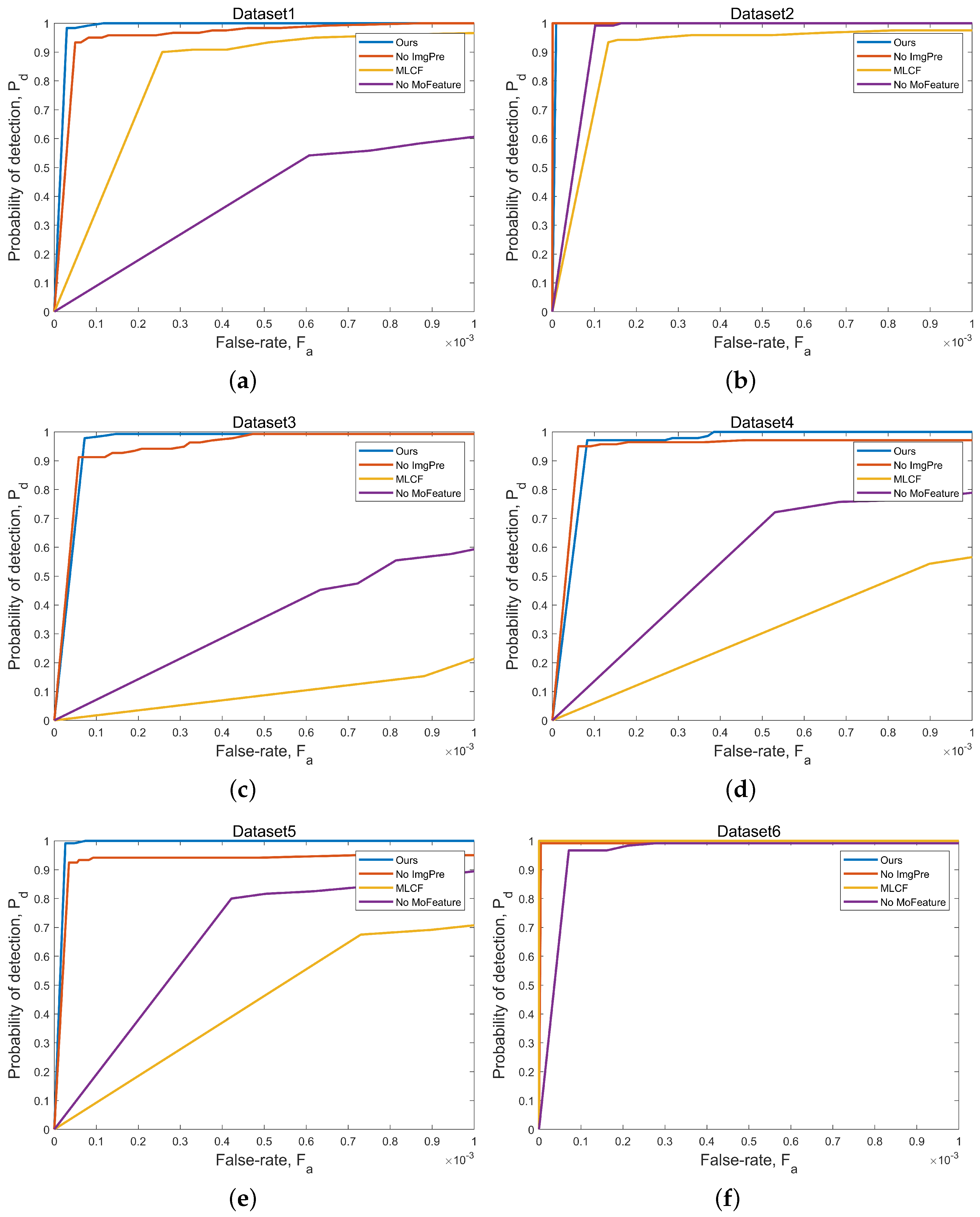
3.2.2. Objective Evaluation

(1) Background Suppression Performance Evaluation
Signal-to-clutter ratio gain (SCRG) and background suppression factor (BSF) are used to characterize the background suppression performance of the method against a complex background [36].
The SCRG is defined as:
S C R = | μ t μ b | σ b
S C R G = S C R o u t S C R i n
where μ t represents the average grayscale value within the target area. μ b and σ b represent the grayscale average and variance of the local background area around the target. S C R o u t and S C R i n represent the processed image and the input image, respectively.
The BSF is defined as:
B S F = δ i n δ o u t
where δ o u t represents the standard deviation of the entire background area of the processed image. δ o u t represents the standard deviation of the entire background area of the input image.
In general, the higher the value of SCRG and BSF, the better the background suppression performance.
The mean values of SCRG and BSF for the six test image sequences are shown in Table 3 and Table 4, respectively. In the tables, the best results for different metrics in different datasets are marked in red. From the experimental results, it can be seen that our algorithm can achieve a better background suppression effect.
As can be seen from the table, our algorithm has better performance regarding its background suppression ability.
(2) Detection Performance Evaluation
ROC curve represents the relationship between detection probability P d and false alarm rate F a , and the area under the curve (AUC) can be calculated for further evaluation of the detection performance. The larger the AUC, the better the detection performance of this method. P d and F a are defined as follows:
P d = N c N r
F a = N f N t
where N c represents the number of correct detections, N r represents the number of real targets, N f represents the number of false detections, and N t represents the total number of pixels detected.
ROC curves of various algorithms obtained on different data are shown in Figure 14. The AUC values are shown in Table 5.
Based on the results presented above, it is apparent that both the ViBe algorithm, which utilizes background modeling, and the MPCM algorithm, which relies on difference-based contrast, demonstrate suboptimal performance in motion detection. The ViBe algorithm utilizes background modeling to compare grayscale differences between the current frame and corresponding pixels in the background, which is constructed based on preceding frames in the sequence. However, in complex scenes, the target’s intensity may be unstable. If the grayscale difference between target pixels and corresponding background pixels in a specific frame fall below the predefined threshold, those pixels are directly classified as a background with a value of 0 in the resulting image. This leads to the algorithm exhibiting the lowest detection rate. Furthermore, as discussed in Section 3.2.1 and evident in Figure 13, when attempting to set a suitable threshold for detecting small and weak targets, there is a higher chance of false positives, incorrectly identifying high-intensity and prominent background elements as targets. The algorithm performs binary classification between targets and background, minimizing the impact of threshold selection on the detection rate and false alarm rate. Consequently, as illustrated in Figure 14, the algorithm’s performance in terms of detection is significantly poor. The MPCM algorithm employs difference-based contrast for background suppression and target enhancement. However, in the presence of weak targets and strong contrast interference, the algorithm tends to suppress the targets as demonstrated in Figure 13. When binary thresholding is applied to the detection results of this algorithm, a high threshold can lead to missed detections, while a low threshold results in excessive false alarms. Overall, this algorithm exhibits a higher rate of missed detections in complex scenes with dim targets. Consequently, the performance of this algorithm, as shown in Figure 14 and Table 5, is unsatisfactory in terms of detection capability. The FMM algorithm employs ratio-based contrast by analyzing the intensity ratio between the target and the surrounding background. Although more robust than MPCM, the FMM algorithm encounters similar challenges, including false positives and background interference that may result in target suppression in specific images. Moreover, the choice of the threshold can lead to problems characterized by missed detections and significant false alarms. Therefore, the performance of this algorithm, as shown by the ROC curve in Figure 14, is somewhat unsatisfactory. Other algorithms do not have significant issues with missed detections, but they are still prone to a higher rate of false alarms due to the influence of the background. However, dataset 6 represents a relatively simple background with significant target intensity and no interference surrounding the target. The NWTH, SR, and IPI algorithms exhibit excellent performance in this environment. Dataset 1 also has a relatively simple background, but it contains noticeable speckles. These algorithms tend to detect these speckles as targets because speckles have similar characteristics to targets in a single-frame image. Consequently, single-frame detection methods relying on spatial features struggle to accurately distinguish targets, leading to an increased incidence of false alarms. Conversely, our algorithm integrates the spatial features of individual frames with the temporal features of consecutive frames to address complex background detection. These two characteristics mutually enhance and mitigate detection errors, thereby achieving precise detections. Thus, our algorithm attains a high detection rate while simultaneously minimizing false alarms.

4. Conclusions

In this paper, we propose a spatio-temporal feature-based algorithm for object detection. For spatial feature-based detection, we introduce MLCF to further exploit the grayscale difference between objects and backgrounds. This enables the identification of sharp grayscale variations, effectively suppressing high-brightness edges and backgrounds with intensity fluctuations, thereby achieving more precise initial object extraction. In the context of temporal feature-based detection, we leverage the STC algorithm, which remains unaffected by pixel grayscale fluctuations and enables the accurate identification of moving targets. The combination of these two features facilitates reliable target extraction and background suppression. Our approach outperforms alternative methods by maintaining high detection accuracy while demonstrating superior background suppression capabilities and a significantly lower false alarm rate. These benefits are particularly valuable when dealing with complex backgrounds featuring prominent interference. Yet, our algorithm still has limitations. The application of a small number of frames for motion detection introduces uncertainties. For instance, consider the case of spots targets. In a small number of frames, there will inevitably be objects that exhibit relative motion to the background but appear stationary relative to the screen. Consequently, these objects may be erroneously identified as spots, leading to missed detections. In our future research, we plan to overcome this limitation by incorporating a larger sequence of frames for long-term tracking. This enhancement will contribute to improved stability in motion feature extraction. On the other hand, our algorithm incorporates temporal features in contrast to single-frame detection algorithms. The motion feature extraction module adopts a global point-by-point tracking approach, which enhances detection capabilities at the cost of real-time performance. During long-term tracking, the computational complexity of the algorithm escalates as more frames are added, exacerbating the impact on real-time performance. As a result, future research will focus on ways to reduce the computational load and enhance the real-time capabilities.

Author Contributions

Conceptualization, Y.W.; Methodology, Y.W.; Formal analysis, K.S.; Resources, N.L. and D.W.; Writing—original draft, Y.W.; Writing—review & editing, K.S. and D.D.; Supervision, L.C. All authors have read and agreed to the published version of the manuscript.

Funding

This research received no external funding.

Data Availability Statement

The data presented in this study are available on request from the corresponding author.

Conflicts of Interest

The authors declare no conflict of interest.

References

  1. Zhou, F.; Wu, Y.; Dai, Y.; Wang, P.; Kang, N. Graph-regularized Laplace approximation for detecting small infrared target against complex backgrounds. IEEE Access 2019, 7, 85354–85371. [Google Scholar] [CrossRef]
  2. Ren, X.; Wang, J.; Ma, T.; Zhu, X.; Bai, K.; Wang, J. Review on Infrared dim and small target detection technology. J. Zhengzhou Univ. (Nat. Sci. Ed.) 2019, 52, 1–21. [Google Scholar]
  3. Bai, X.; Bi, Y. Derivative Entropy-based Contrast Measure for Infrared Small-target Detection. IEEE Trans. Geosci. Remote Sens. 2018, 56, 2452–2466. [Google Scholar] [CrossRef]
  4. Li, J.; Zhang, P.; Wang, X.; Huang, S. Infrared Small-target Detection Algorithms: A Survey. J. Image Graph. 2020, 25, 1739–1753. [Google Scholar]
  5. Deng, H.; Sun, X.; Zhou, X. A Multiscale Fuzzy Metric for Detecting Small Infrared Targets Against Chaotic Cloudy/Sea-Sky Backgrounds. IEEE Trans. Cybern. 2019, 45, 1694–1707. [Google Scholar] [CrossRef] [PubMed]
  6. Kim, S. Target attribute-based false alarm rejection in small infrared target detection. Proc. SPIE 2012, 8537, 85370G. [Google Scholar]
  7. Yang, W.; Shen, Z. Preprocessing Technology for Small Target Detection in Infrared Image Sequences. Infrared Laser Eng. 1998, 27, 23–28. [Google Scholar]
  8. Suyog, D.D.; Meng, H.E.; Ronda, V.; Philip, C. Max-mean and max-median filters for detection of small targets. Proc. SPIE 1999, 3809, 74–83. [Google Scholar]
  9. Bae, T.W.; Sohng, K.I. Small Target Detection Using Bilateral Filter Based on Edge Component. J. Infrared Millim. Terahertz Waves 2010, 31, 735–743. [Google Scholar] [CrossRef]
  10. Yuan, C.; Yang, J.; Liu, R. Detecting Infrared Small Target By Using TDLMS Filter Baesd on Neighborhood Analysis. J. Infrared Millim. Waves 2009, 28, 235–240. [Google Scholar]
  11. Han, J.; Wei, Y.; Peng, Z.; Zhao, Q.; Chen, Y.; Qin, Y.; Li, N. Infrared dim and small target detection: A review. Infrared Laser Eng. 2022, 51, 20210393. [Google Scholar]
  12. Yang, L.; Yang, J.; Yang, K. Adaptive detection for infrared small target under sea-sky complex background. Electron. Lett. 2004, 40, 1083–1085. [Google Scholar] [CrossRef]
  13. Liu, Z.; Yang, D.; Li, J.; Huang, C. A review of infrared single frame dim small target detection algorithms. Laser Infrared 2022, 52, 154–162. [Google Scholar]
  14. Candès, E.J.; Li, X.; Ma, Y.; John, L. Robust principal component analysis. J. ACM 2011, 58, 1–37. [Google Scholar] [CrossRef]
  15. Fan, J.; Gao, Y.; Wu, Z.; Li, L. Detection Algorithm of Single Frame Infrared Small Target Based on RPCA. J. Ordnance Equip. Eng. 2018, 39, 147–151. [Google Scholar]
  16. Gao, C.; Meng, D.; Yang, Y.; Wang, Y.; Zhou, X.; Alexander, G.H. Infrared patch-image model for small target detection in a single image. IEEE Trans. Image Process. 2013, 22, 4996–5009. [Google Scholar] [CrossRef] [PubMed]
  17. Zhang, T.; Wu, H.; Liu, Y.; Peng, L.; Yang, C.; Peng, Z. Infrared Small Target Detection Based on Non-Convex Optimization with Lp-Norm Constraint. Remote Sens. 2019, 11, 559. [Google Scholar] [CrossRef]
  18. Zhou, F.; Wu, Y.; Dai, Y.; Wang, P. Detection of Small Target Using Schatten 1/2 Quasi-Norm Regularization with Reweighted Sparse Enhancement in Complex Infrared Scenes. Remote Sens. 2019, 11, 2058. [Google Scholar] [CrossRef]
  19. Li, C.; Zhang, B.; Hong, D.; Yao, J.; Jocelyn, C. LRR-Net: An Interpretable Deep Unfolding Network for Hyperspectral Anomaly Detection. IEEE Trans. Geosci. Remote Sens. 2023, 61, 5513412. [Google Scholar] [CrossRef]
  20. Itti, L.; Koch, C.; Niebur, E. A model of saliency-based visual attention for rapid scene analysis. IEEE Trans. Pattern Anal. Mach. Intell. 1998, 20, 1254–1259. [Google Scholar] [CrossRef]
  21. Kim, S.; Yang, Y.; Lee, J.; Park, Y. Small target detection utilizing robust methods of the human visual system for IRST. J. Infrared Millim. Terahertz Waves 2009, 30, 994–1011. [Google Scholar] [CrossRef]
  22. Wang, X.; Lv, G.; Xu, L. Infrared dim target detection based on visual attention. Infrared Phys. Technol. 2012, 55, 513–521. [Google Scholar] [CrossRef]
  23. Han, J.; Ma, Y.; Huang, J.; Mei, X.; Ma, J. An infrared small target detecting algorithm based on human visual system. IEEE Geosci. Remote Sens. Lett. 2016, 13, 452–456. [Google Scholar] [CrossRef]
  24. Chen, C.; Li, H.; Wei, Y.; Tian, X.; Yuan, Y. A local contrast method for small infrared target detection. IEEE Trans. Geosci. Remote Sens. 2014, 52, 574–581. [Google Scholar] [CrossRef]
  25. Han, J.; Ma, Y.; Zhou, B.; Fan, F.; Kun, L.; Yu, F. A robust infrared small target detection algorithm based on human visual system. IEEE Geosci. Remote Sens. Lett. 2014, 11, 2168–2172. [Google Scholar]
  26. Qin, Y.; Li, B. Effective infrared small target detection utilizing a novel local contrast method. IEEE Geosci. Remote Sens. Lett. 2016, 13, 1890–1894. [Google Scholar] [CrossRef]
  27. Wu, X.; Hong, D.; Jocelyn, C. UIU-Net: U-Net in U-Net for Infrared Small Object Detection. IEEE Trans. Image Process. 2022, 32, 364–376. [Google Scholar] [CrossRef] [PubMed]
  28. Zhou, Y.; Liu, H.; Ma, F.; Pan, Z.; Zhang, F. A Sidelobe-Aware Small Ship Detection Network for Synthetic Aperture Radar Imagery. IEEE Trans. Geosci. Remote Sens. 2023, 61, 5205516. [Google Scholar] [CrossRef]
  29. Wu, X.; Hong, D.; Tian, J.; Jocelyn, C.; Li, W.; Ran, T. ORSIm Detector: A Novel Object Detection Framework in Optical Remote Sensing Imagery Using Spatial-Frequency Channel Features. IEEE Trans. Geosci. Remote Sens. 2019, 57, 5146–5158. [Google Scholar] [CrossRef]
  30. Kim, S.; Sun, S.G.; Kim, K.T. Highly efficient supersonic small infrared target detection using temporal contrast filter. Electron. Lett. 2014, 50, 81–83. [Google Scholar] [CrossRef]
  31. Lin, H.; Chuang, J.; Liu, T. Regularized background adaptation: A novel learning rate control scheme for Gaussian mixture modeling. Image Process. IEEE Trans. 2011, 20, 822–836. [Google Scholar]
  32. Kim, K.; Thanarat, H.C.; David, H.; Larry, D. Real-time Foreground-Background Segmentation using Codebook Model. Real-Time Imaging 2005, 11, 167–256. [Google Scholar] [CrossRef]
  33. Cheng, K.; Hui, K.; Zhan, Y.; Qi, M. A novel improved ViBe algorithm to accelerate the ghost suppression. In Proceedings of the 12th International Conference on Natural Computation, Fuzzy Systems and Knowledge Discovery, Changsha, China, 13–15 August 2016; pp. 1692–1698. [Google Scholar]
  34. Berthold, K.P.H.; Brian, G.S. Determining optical flow. Artif. Intell. 1981, 1, 185–203. [Google Scholar]
  35. Bruce, D.L.; Takeo, K. An iterative image registration technique with an application to stereo vision. In Proceedings of the 7th International Joint Conference on Artificial Intelligence—Volume 2 (IJCAI’81), San Francisco, CA, USA, 24–28 August 1981; Morgan Kaufmann Publishers Inc.: San Francisco, CA, USA, 1981; pp. 674–679. [Google Scholar]
  36. Ma, Y.; Liu, Y.; Pan, Z.; Hu, Y. Method of Infrared Small Moving Target Detection Based on Coarse-to-Fine Structure in Complex Scenes. Remote Sens. 2023, 15, 1508. [Google Scholar] [CrossRef]
  37. Jiang, Y.; Dong, L.; Yang, C.; Xu, W. An infrared small target detection algorithm based on peak aggregation and Gaussian discrimination. IEEE Access 2020, 8, 106214–106225. [Google Scholar] [CrossRef]
  38. Wu, L.; Ma, Y.; Fan, F.; Wu, M.; Huang, J. A Double-Neighborhood Gradient Method for Infrared Small Target Detection. IEEE Geosci. Remote Sens. Lett. 2021, 18, 1476–1480. [Google Scholar] [CrossRef]
  39. Zhang, K.; Zhang, L.; Yang, M.; Zhang, D. Fast Tracking via Spatio-Temporal Context Learning. arXiv 2013, arXiv:1311.1939. [Google Scholar]
  40. Hui, B.; Song, Z.; Fan, H.; Zhong, P.; Hu, W.; Zhang, X.; Ling, J.; Su, H.; Jin, W.; Zhang, Y.; et al. A dataset for infrared image dim-small aircraft target detection and tracking under ground/air background. Sci. Data Bank 2019, 5, 291–302. [Google Scholar]
  41. Bai, X.; Zhou, F. Analysis of new top-hat transformation and the application for infrared dim small target detection. Pattern Recognit. 2010, 43, 2145–2156. [Google Scholar] [CrossRef]
  42. Wei, Y.; You, X.; Li, H. Multiscale patch-based contrast measure for small infrared target detection. Pattern Recognit. 2016, 58, 216–226. [Google Scholar] [CrossRef]
  43. Hou, X.; Zhang, L. Saliency Detection: A Spectral Residual Approach. In Proceedings of the 2007 IEEE Conference on Computer Vision and Pattern Recognition, Minneapolis, MN, USA, 17–22 June 2007; pp. 1–8. [Google Scholar]
  44. Olivier, B.; Marc, V.D. ViBe:A universal background subtraction algorithm for video sequences. IEEE Trans. Image Process. 2011, 20, 1709–1724. [Google Scholar]
Figure 1. The flowchart of the moving small target detection algorithm.
Remotesensing 15 05380 g001
Figure 2. The image is filtered by a LoG and DoG; (a) the original image and (b) the image smoothed by the LoG filter kernel, (c) the image smoothed by the DoG filter kernel.
Remotesensing 15 05380 g002
Figure 3. The resulting local significance graph.
Remotesensing 15 05380 g003
Figure 4. Target enhancement result diagram, (a) the original image, (b) the 3D view of the original image, (c) the enhanced image, (d) the enhanced 3D view. The X and Y axes in the 3D views of (b) and (d) depict the row and column coordinates of the image, respectively. The Z axis represents the grayscale value of the pixels associated with the image coordinates, and the range of pixel grayscale values is from 0 to 255. Their scr values can be seen in Equation (11).
Remotesensing 15 05380 g004
Figure 5. (a,c) The original image and (b,d) the LCM image.
Remotesensing 15 05380 g005
Figure 6. Three-layer window model introduction, (a) our structure, and (b) the structure of DNGM.
Remotesensing 15 05380 g006
Figure 7. (a) The original drawing, (b) the detection results through 3 × 3 LCF, and (c) the detection results through 3 × 3 DNGM.
Remotesensing 15 05380 g007
Figure 8. Model diagram of of the spatial relationship between an object and its local context. The local context region Ω c is inside the grayish blue rectangle that is included to trace the result, the area of the object around which the red rectangle is centered. Context features at position z are represented by c ( z ) = ( I ( z ) , z ) and include low-level appearance representations (i.e., image intensity I ( z ) ) and location information.
Remotesensing 15 05380 g008
Figure 9. Cross section of the confidence map of Different parameters β . The target coordinates here are x * = ( 100 , 100 ) . The horizontal axis represents the row or column coordinates of the image, while the vertical axis represents the confidence value at different coordinates centered around point x * .
Remotesensing 15 05380 g009
Figure 10. (a) The motion vector of global pixels, (b) (top) the motion vector of the target and nearby pixels, and (b) (below) the motion vector of background pixels.
Remotesensing 15 05380 g010
Figure 11. (a) The AMF, and (b) the 3D view of AMF.
Remotesensing 15 05380 g011
Figure 12. (af) The ROC curves of the detection results obtained from the ablation experiments on various datasets are presented. Images (af) correspond to dataset 1–dataset 6, respectively. The horizontal axis represents the false alarm rate, while the vertical axis represents the detection rate. Different curves within the same dataset correspond to different experimental workflows.
Remotesensing 15 05380 g012
Figure 13. Original image data, processing results and 3D view, in which (IVI) is corresponding to dataset1–dataset6, respectively, (a1) in each group is the original data, (b1h1) is the result of different processing methods, and (a2) is the 3D graph of the original data. (b2h2) correspond to the grayscale 3D maps of the results of different processing methods in turn, where the real target area is marked in red. The corresponding results of the target detection are shown in the figure. Among them, the correctly detected target areas are marked in green, and the missed target areas are marked in blue. In addition, obvious false alarm areas are marked in yellow, while less obvious false alarm areas are not marked.
Remotesensing 15 05380 g013aRemotesensing 15 05380 g013bRemotesensing 15 05380 g013cRemotesensing 15 05380 g013d
Figure 14. ROC curves calculated on each datum. Images (af) correspond to dataset 1–dataset 6, respectively. Within each group of images, the different colored curves represent different algorithms. The horizontal axis represents the false alarm rate, while the vertical axis represents the detection rate.
Remotesensing 15 05380 g014
Table 1. Details of the datasets.
DatasetsFramesSizeTarget SizeBackground
Dataset 1120256 × 2562 × 2Roads and buildings, with camera spots and obvious performance
Dataset 2100256 × 2562 × 2Woods and Roads
Dataset 3120256 × 2561 × 1–2 × 2Woods and roads, presence of background interference from suspected target
Dataset 4120256 × 2562 × 2Mountains and roads, camera spots exist
Dataset 5100256 × 2562 × 2–3 × 3Woods and buildings, the presence of background interference from suspected targets
Dataset 6120256 × 2562 × 2Sky and buildings, there are camera spots and mostly fall in the construction area
Table 2. Algorithm and its parameter settings.
MethodParameters
NWTH [37] R o = 6,    R i = 4
MPCM [38]Size = 3 × 3,   5 × 5,   7 × 7
FMM [5]Size = 3 × 3
SR [39]Filter size = 3 × 3
ViBe [40]Sample size N = 20,   threshold min = 2,   distance decision threshold R = 20
IPI [16]Window = 20 × 20,   step = 10
OursSize = 3 × 3,   5 × 5,   7 × 7,   sz = 55 × 55
Table 3. SCRG values of each data and method.
Data 1Data 2Data 3Data 4Data 5Data 6
NWTH5.59038.15472.13141.48063.43847.1288
MPCM6.344413.76792.80511.39864.191238.3163
FMM15.015123.34088.46427.701311.65826.1281
SR46.54578.300520.685818.957341.317864.6102
ViBe26.986926.30323.99636.84036.55310.9571
IPI0.3630.42140.34610.30640.23830.3972
Ours450.3183557.0121278.7068263.6374180.7475160.8375
Table 4. BSF values for each data and method.
Data 1Data 2Data 3Data 4Data 5Data 6
NWTH3.76154.782.4092.53653.780618.0906
MPCM3.27473.12132.47373.01586.675713.0021
FMM2.3571.99511.85061.61322.29145.7597
SR3.11523.86471.69851.6442.0956.8911
ViBe2.69483.24213.46883.17474.8472.9726
IPI2.09862.29841.52151.57292.06065.3225
Ours89.2149329.165329.114935.647560.3617185.2471
Table 5. AUC values of each datum and processing method.
Datum 1Datum 2Datum 3Datum 4Datum 5Datum 6
NWTH0.97640.85530.99150.96030.98471
MPCM0.55680.14110.55540.38250.81280.1125
FMM0.85260.67270.95100.90120.98750.6439
SR0.92180.97430.96470.96420.98040.9839
ViBe0.33660.47550.67230.55060.61890.3824
IPI0.98700.98590.97030.98480.99430.9944
Ours0.99840.99540.99950.99950.99990.9983
Disclaimer/Publisher’s Note: The statements, opinions and data contained in all publications are solely those of the individual author(s) and contributor(s) and not of MDPI and/or the editor(s). MDPI and/or the editor(s) disclaim responsibility for any injury to people or property resulting from any ideas, methods, instructions or products referred to in the content.

