An Automatic Deep Learning Bowhead Whale Whistle Recognizing Method Based on Adaptive SWT: Applying to the Beaufort Sea

Abstract

The bowhead whale is a vital component of the maritime environment. Using deep learning techniques to recognize bowhead whales accurately and efficiently is crucial for their protection. Marine acoustic remote sensing technology is currently an important method to recognize bowhead whales. Adaptive SWT is used to extract the acoustic features of bowhead whales. The CNN-LSTM deep learning model was constructed to recognize bowhead whale voices. Compared to STFT, the adaptive SWT used in this study raises the SCR for the stationary and nonstationary bowhead whale whistles by 88.20% and 92.05%, respectively. Ten-fold cross-validation yields an average recognition accuracy of 92.85%. The method efficiency of this work was further confirmed by the consistency found in the Beaufort Sea recognition results and the fisheries ecological study. The research results in this paper help promote the application of marine acoustic remote sensing technology and the conservation of bowhead whales.

1. Introduction

The bowhead whale is a crucial marine ecosystem component and plays a key role in the Arctic’s marine food chain, energy flow and ecological balance [1,2]. In recent years, the survival of the bowhead whale has been seriously threatened due to human activities such as the exploration of submerged resources, the expansion of shipping and the use of artificial sonar [3,4]. Recognizing, analyzing and researching the bowhead whale voice is essential for comprehending bowhead whale habitat behaviors and habits [5]. As a traditional field of remote sensing, ocean acoustic remote sensing technology has advanced significantly in recent years [6,7,8,9,10,11]. Ocean acoustic remote sensing technology can monitor whale habitats, track whale behaviors [12] and detect whale strandings [13] and other whale-related incidents. Consequently, recognizing the bowhead whale voice using remote sensing technology in the marine environment has become a top priority.

The application of ocean acoustic remote sensing technology is currently the mainstream method for recognizing bowhead whales [14]. These acoustic remote sensing data recognize bowhead whales primarily using a passive acoustic monitoring (PAM) system [15,16]. Over a lengthy period, PAM has amassed enormous data information [17] and is limited to a number of trained and experienced individuals. Moreover, the bowhead whale voice contains broadband stationary and nonstationary components [18]. Because of these, it is extremely inefficient to manually recognize bowhead whale voices [19] and difficult to ensure real-time and precise recognition. As a result, there is an immediate need for a precise method to automatically recognize bowhead whale voices so as to comprehend bowhead whale behaviors, population structures and migration patterns to protect bowhead whale species and preserve the stability and diversity of marine ecosystems.

The recognition effect of bowhead whale voices hinges on the efficient extraction of target features and the design of classifiers [20]. Currently, traditional feature extraction methods such as the short-time Fourier transform (STFT) [21,22,23,24], wavelet transform (WT) [23,25,26], Winger-Ville distribution (PWVD) [27] and Hilbert–Huang Transform (HHT) [28] are used for bowhead whale voice recognition. All of the above methods have their shortcomings in terms of time-frequency feature extraction, which are summarized below. The time-frequency resolution of STFT and WT is dependent on the choice of window and basis function. Therefore, they are ineffective at matching voices with multiple time-varying components. The WVD is not noise-resistant and includes cross-interference factors for multicomponent voices. The distribution of transform coefficients in the time-frequency plane of conventional methods is relatively discrete as a result. In other terms, the time-frequency curve’s amplitude energy is not sufficiently centralized. In order to improve time-frequency aggregation, the present research focuses on energy rearrangement based on the original time-frequency spectrum. In 2011, Daubechies et al. proposed the synchrosqueezed wavelet transform (SWT) [29], which enables high-resolution representation of complex multicomponent signals. However, SWT has not been used to recognize whale voices in previous studies. Since the selection of wavelet parameters will affect the quality of time-frequency aggregation, this paper applies adaptive SWT to extract bowhead whale voice features to make the recognition result more accurate. The advancement of artificial intelligence makes it feasible to recognize ocean acoustic signals efficiently and rapidly using deep learning techniques. Deep learning techniques have enabled the effective and quick recognition of maritime acoustic waves thanks to advancements in artificial intelligence [30,31,32,33,34]. Several automatic identification and classification methods have been used for whale sound recognition. Among them, CNN has been used by many researchers for whale voice recognition due to its power in image recognition [35,36,37]. However, most studies have only utilized the spatial feature extraction capability of CNNs, ignoring the continuity of whale voices. Shaym Madhusudhana [38,39] explored the prospect of utilizing the temporal context inherent in the songs of fin whales (Balaenoptera physalus) to improve the performance of automatic recognition and demonstrated that the incorporation of temporal information improves the automatic recognition and transcription of wildlife recordings. Considering the continuity of bowhead whale sounds in the temporal direction, a CNN-LSTM intelligent learning model was constructed to improve the accuracy of bowhead whale whistle recognition. The combination of CNN and LSTM captured the spatial and temporal features of bowhead whale sounds.

Due to the complexity of the marine environment and the diversity of bowhead whale voices, there is no fully dependable feature extraction and recognition method that can achieve accurate detection, recognition and classification of bowhead whale voices. Manual classification methods are still the primary means of recognizing and classifying bowhead whale acoustic signals at present. Research on automatic recognition and classification methods of bowhead whale acoustic signals between species with high classification accuracy, significant generalization ability and recognition of many species is still an important research content in the current field of marine acoustics. Developing a classification method that can effectively extract signal features and adaptively learn signal differences while adapting new features from new data is an essential development direction for marine mammal acoustic signal classification.

The goal of this paper is to accurately recognize bowhead whale whistles by employing an adaptive SWT feature extraction method and building CNN-LSTM deep learning models. The main contributions of this work are the following: (1) Using ocean acoustic remote sensing technology to extract the features of bowhead whale voices using adaptive SWT. To quantify and compare the performance of this paper’s method with other traditional feature extraction methods by average SCR metrics. (2) Recognizing the bowhead whale voices automatically using CNN-LSTM. Incorporation of the temporal contextual information provided by the LSTM network for recognition of bowhead whales. This model combines the CNN’s potent spatial feature extraction capability and the temporal voice processing advantage of the LSTM, which further makes full use of ocean acoustic remote sensing data and promotes the development of ocean acoustic remote sensing technology in marine ecological protection.

The main structure of this paper is as follows. Section 2 describes the relevant experimental data and its preprocessing, the experimental methodology and the construction of the model. Section 3 presents the experimental results of this paper. In Section 4, the methodology of this paper is applied to the measured data in the Beaufort Sea. Section 5 describes the limitations of this paper and future research directions and the conclusions are presented in Section 6.

2. Materials and Methods

2.1. Dataset

The dataset in this paper consists of two parts. One from the Watkins and DRYAD databases for essential feature labeling and model training and another from the Beaufort Sea PAM stations in the Arctic for validating the methodology. These datasets are explicitly introduced in the following.

• Watkins: This dataset consists of 60 recording files of the bowhead whale voices from the Bering Strait, Barrow, Alaska. The bowhead whale voice information is shown in

  Table 1. Information from Watkins database.

  Number	Sampling Freq (Hz)	Whale Frequency Band
  1	10,240	100–4000
  2	10,240	500–3000
  3	10,240	200–2000
  4	10,000	100–3000
  5	10,000	100–2500
  6	10,000	200–2000
  ……	……	……
  55	10,240	50–2000
  56	10,000	100–500
  57	10,000	50–2500
  58	10,000	100–3500
  59	10,240	500–4500
  60	10,000	450–3000

  . Column 2 describes the sampling frequency of bowhead whale voices; column 3 describes the bowhead whale voices band range.
• DRYAD: This dataset is derived from 184 sound clips recorded over three consecutive winters in the Fram Strait by Stafford et al. [40]. Of these, 38 singing segments were identified in 2010–2011; 69 segments were identified in 2012–2013 and 76 segments were identified in 2013–2014.
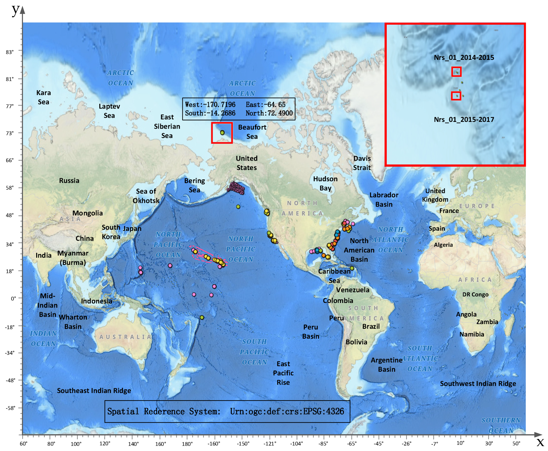
• NOAA PAM: This dataset is from the National Oceanic and Atmospheric Administration’s National Centers for Environmental Information Arctic Beaufort Sea PAM station, which was used to validate the methodology in this paper. The PAM sites in the Beaufort Sea and related information are depicted in Figure 1. The measured recording size is 23.3 M.

2.2. Data Analysis

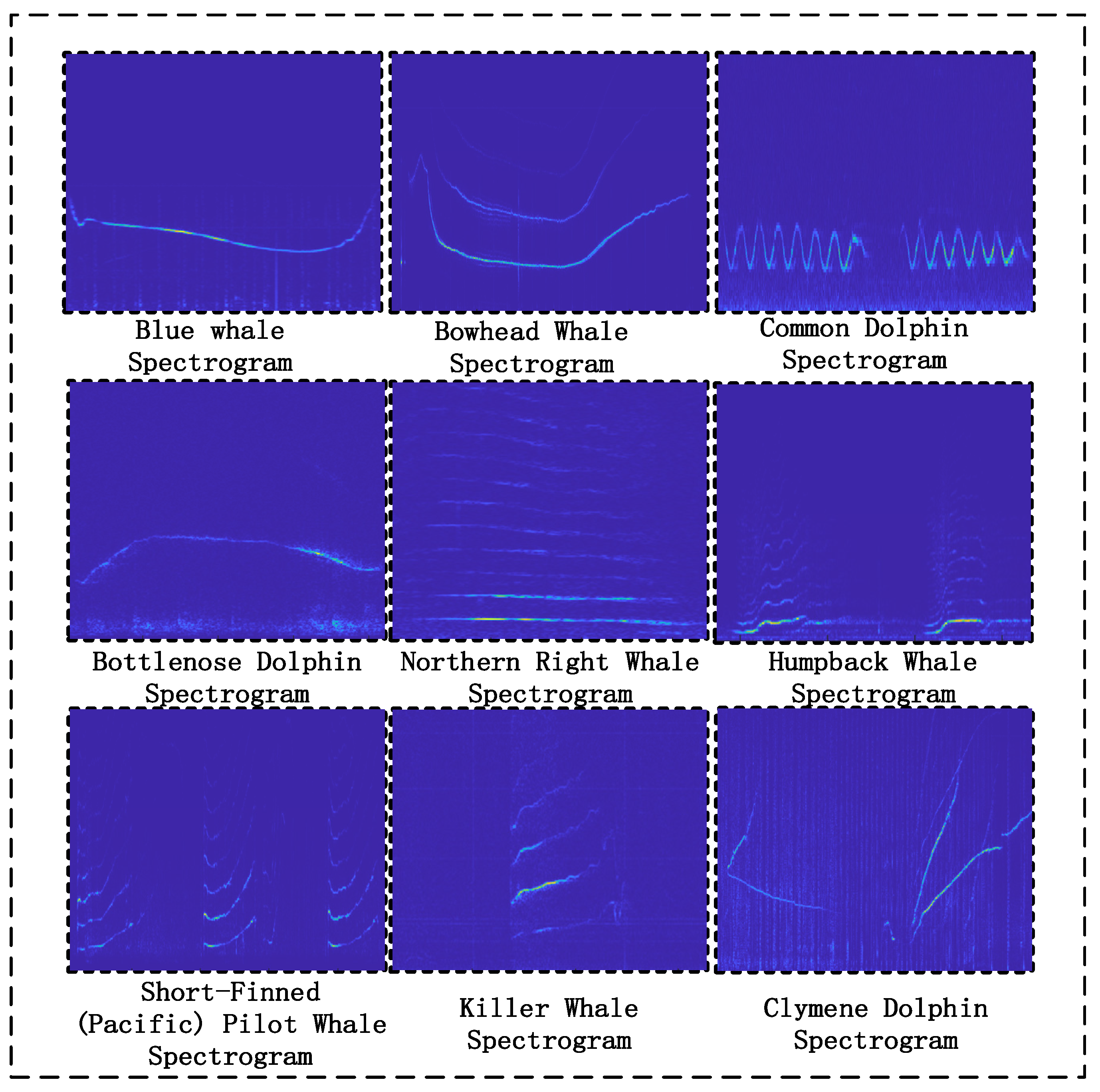
2.2.1. Bowhead Whale Voice Characteristics

Bowhead whale voices, like in the case of other whales (Figure 2), are characterized by low frequencies and complexity. Among them, bowhead whale whistles are primarily used for social interaction and communication. Multiple researchers [40,41] have provided evidence of a strong association between bowhead whale whistles and abundance through vocal and visual comparisons. It also provides theoretical support for the feature labeling of bowhead whale voice datasets. Therefore, recognizing bowhead whales by whistles is currently the most reliable way.

Table 2. The main acoustic characteristics of bowhead whales summarized by Erbs F et al.

Type	Subtype	Min f (Hz)	Max f (Hz)	Delta f (Hz)	Start f (Hz)	End f (Hz)	Med f (Hz)	Delta Time (S)
M		1055	2160	1105	1724	1142	1672	8.46
	MSG1	1077	2069	1532	2002	1122	2012	14.1
	MSG5	762	2586	1823	1817	820	1894	10.5
	MSG11	1271	1771	501	1722	1438	1512	9.09
	MSG2	1163	2246	1083	1962	1225	1923	8.84
	Mo	1046	2015	1060	1654	1125	1598	7.63
S		461	872	410	593	803	728	1.4
Vigh		973	1605	631	1461	1155	1095	1
rumble		234	319	84	278	272	279	7.3
	Short R	221	298	76	265	258	257	4.5
	Long R	266	370	104	309	306	331	14
sLFdown		83	202	119	180	110	147	0.0
sLFconst		341	412	71	383	370	376	0.3
sLFconst2		589	713	123	673	623	627	0.1
Minter		869	1153	284	1135	917	1049	0.6
	MiSG3	1137	1276	139	1254	1184	1198	1.2
	Mio	708	1079	370	1064	758	958	0.3
sup		457	537	80	481	520	504	0.0

presents the primary acoustic characteristics of the nine unit types of bowhead whales, which is quoted from Erbs et al. [41]. Each column of title from left to right in Table 2 represents minimum frequency, maximum frequency, frequency bandwidth, frequency start, frequency end, median frequency and bandwidth duration.

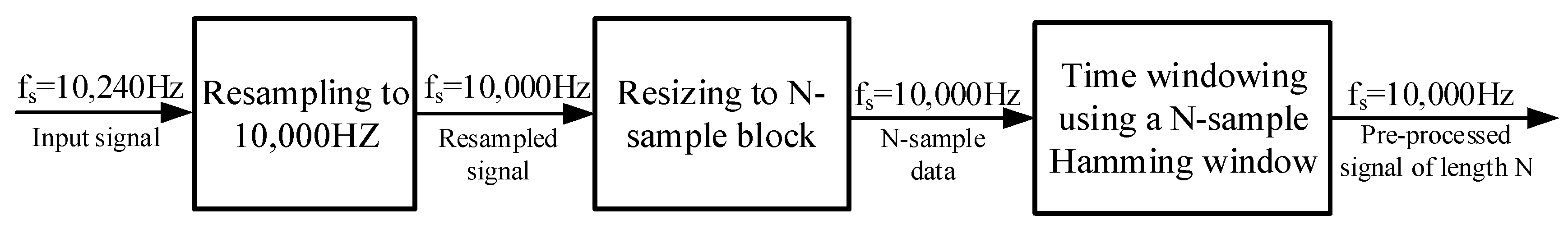
2.2.2. Data Processing

The data are preprocessed for the following algorithms to process them more effectively. Firstly, we resampled all recordings to a fixed sampling rate of 10,000 Hz. Then, according to Bu Lingran et al. [42], we frame the resampled data segments into blocks with a length of $N=\mathrm{25,000} (2.5 \mathrm{s})$ and added the Hamming window. Figure 3 depicts the data preprocessing structure. The data preprocessing in this section decreases the computational complexity of the subsequent processes and conserves computer memory.

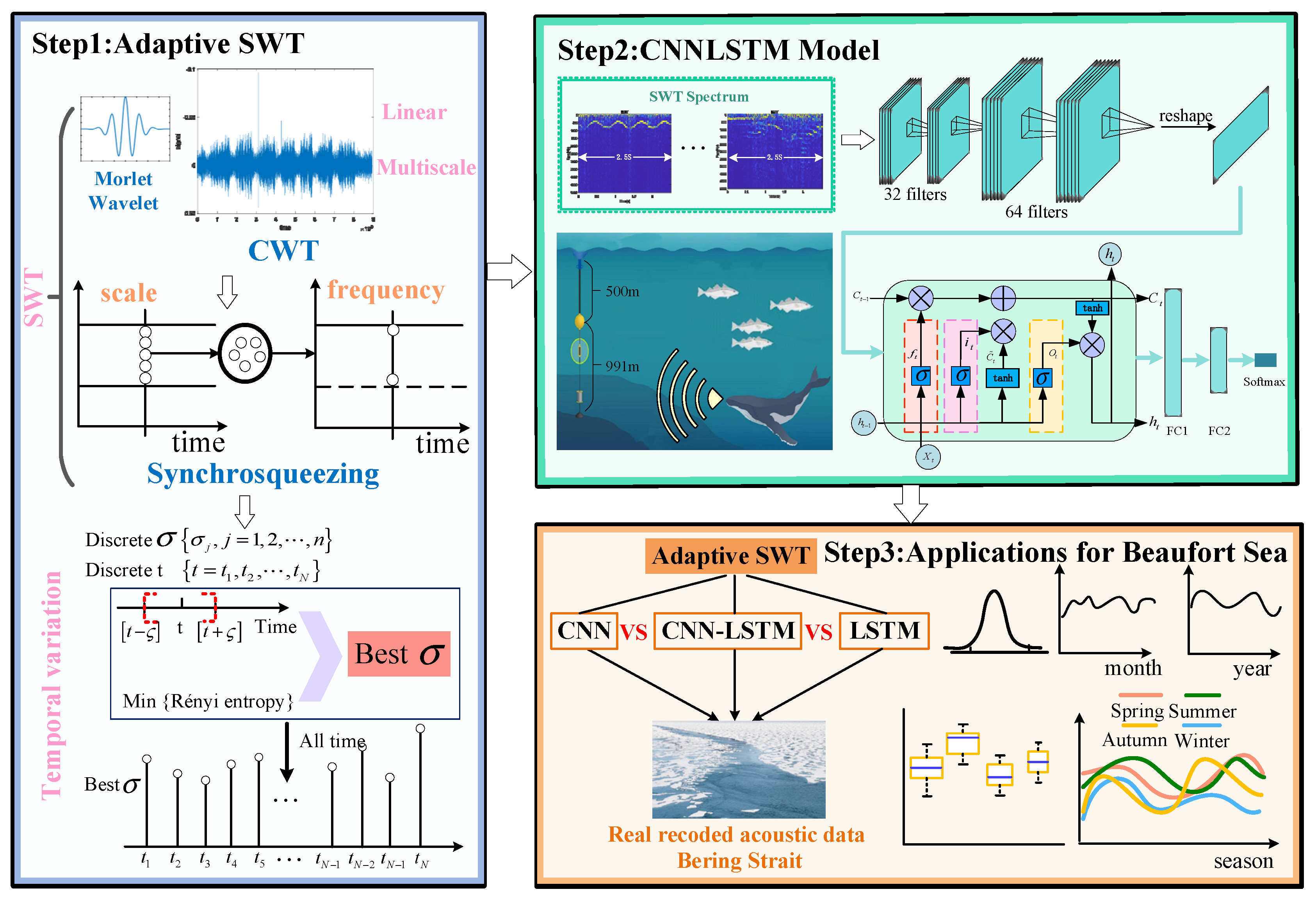
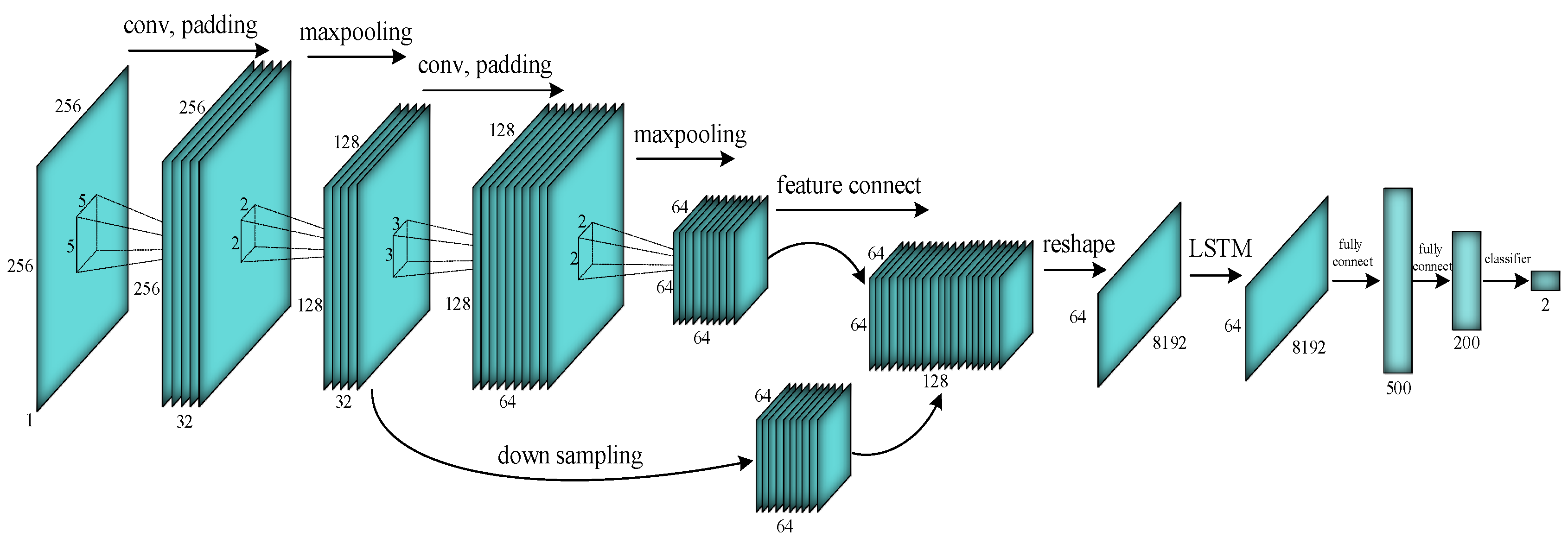
2.3. Model Architecture

This paper’s architecture of recognizing bowhead whale whistles using adaptive SWT and CNN-LSTM includes three stages, as depicted in Figure 4.

Step 1: Proposing adaptive SWT, compressing and rearranging the voice’s time-frequency coefficients, determining the optimal wavelet parameters by traversing each moment and obtaining the time-frequency diagrams based on the optimal time-varying parameters.

Step 2: Constructing the CNN-LSTM model. Connecting CNN and LSTM models through dimensional merging and transformation techniques. The model consists of two convolutional layers, maximum pooling and fully connected layers. In the convolutional layer, the SWT spectrum is used as the input to extract the spatial domain features of the signal. Through the gate mechanism, the time domain characteristics of the signal are preserved. Then, the results are compared to those of artificial specialists in the fully connected layer.

Step 3: Completing the comparison experiments, solidifying the model presented in this paper and applying it to the measured data of the Beaufort Sea. Comparing the model presented in this paper to STFT, CNN, LSTM and other models. Then, employing the model to PAM data from the Beaufort Sea, we analyzed the seasonal and interannual variation in bowhead whales from 2014 to 2017 in the Beaufort Sea. The results of this paper were compared to fishery ecology studies to validate the veracity of this paper’s methodology.

2.4. Feature Extraction

2.4.1. Bowhead Whale Whistle Feature Extraction Based on SWT

Inspired by the Empirical Mode Decomposition (EMD) adaptive decomposition method, Daubechies, one of the founders of the wavelet transform, proposed the synchrosqueezed wavelet transform (SWT) in 2011 [29]. The main idea of SWT is to redistribute the wavelet transform coefficients to the estimated instantaneous frequency and improve the time-frequency resolution and frequency of the signal energy concentration. The implementation of this technology mainly includes the following three steps [29]:

(1)

Select the appropriate wavelet basis function and perform continuous wavelet transform on the original signal.

The Morlet wavelet has a simple mathematical representation and good localization ability in both the time and frequency domains. Therefore, we choose the Morlet wavelet as the wavelet basis function. Assuming $\mathsf{\psi }\left(t\right)$ is the Morlet wavelet, in the time domain, the Morlet wavelet can be expressed as:

$$\mathsf{\psi }\left(t\right)=\frac{1}{\sigma \sqrt{2\pi }}{e}^{-{\left(\frac{1}{\sqrt{2}\sigma }\right)}^2}\left(e^{i2\pi \mu t}-e^{-2{\pi }^2{\sigma }^2{\mu }^2}\right)$$

(1)

Then, the time domain continuous wavelet transform of the signal $x\left(t\right)$ is:

$$\mathrm{W}\left(a,b\right)=\int \mathrm{x}\left(t\right)a^{-1/2}\mathsf{\psi }\left(\frac{t-b}{a}\right)dt$$

(2)

Among them, $\sigma >0$, $\mu >0$, $\sigma$ is a wavelet parameter to adjust the window width and has a certain influence on the time-frequency concentration [43]. $\mu$ is the center of frequency, $x\left(t\right)$ is the original signal, $\mathrm{W}\left(a,b\right)$ is the result of the continuous wavelet transform of $x\left(t\right)$, $t$ is the time, $a$ is the scale factor, b is the time factor, a is discretized by power series and b is discretized uniformly, covering the entire time axis. $\psi \left(t\right)$ is the complex conjugate function of the wavelet basis function. Combined with Plancherel’s theorem, we can get the frequency domain wavelet transform result as:

$${\mathrm{W}}_f\left(a,b\right)=\frac{1}{\sqrt{2\pi }}\int \widehat{x}\left(\epsilon \right)a^{1/2}\widehat{\mathsf{\psi }}\left(a\epsilon \right)e^{ib\epsilon }d\epsilon$$

(3)

where $\epsilon$ is the angular frequency, $\widehat{x}\left(\epsilon \right)$ and $\widehat{\psi }\left(\epsilon \right)$ are the Fourier transform results of $x\left(t\right)$ and $\psi \left(t\right)$, and $i=\sqrt{-1}$ represents the imaginary number.

(2)

Calculate the instantaneous frequency of the original signal.

Since the signal’s phase is stable and does not change with the scale factor change, its instantaneous frequency can be obtained by calculating the phase partial derivative of the signal.

$${\mathsf{\omega }}_f\left(a,b\right)=-i\left[\frac{\partial }{\partial b}{\mathrm{W}}_f\left(a,b\right)\right]/{\mathrm{W}}_f\left(a,b\right)dt$$

(4)

(3)

Compress and reorganize the wavelet coefficients in the frequency direction to obtain the synchronously compressed wavelet transform $\mathrm{T}\left(a,b\right)$.

Transform the wavelet transform coefficients from the time-scale domain to the time-frequency domain and compress them in the frequency domain. At this moment, the frequency variable $\omega$ and the scale factor $a$ are discretized. Compress and reorganize the value of $\left[{\mathsf{\omega }}_{\mathrm{c}}-∆\mathsf{\omega }/2,{\mathsf{\omega }}_{\mathrm{c}}+∆\mathsf{\omega }/2\right]$ near any center frequency ${\omega }_c$ of ${\mathrm{W}}_f\left[{\mathsf{\omega }}_f\left(a,b\right),b\right]$ so that the area where the wavelet coefficients diverge from the frequency direction is compressed to near the center frequency, thereby greatly improving the frequency resolution.

In the actual processing of the whale signal, all the discrete values in the time domain are obtained, so the scale needs to be discretized and the synchronous compression wavelet transform result $\mathrm{T}\left({\mathsf{\omega }}_c,b\right)$ of the whale signal can be expressed as:

$$\mathrm{T}\left({\mathsf{\omega }}_c,b\right)=\left(1/∆{\mathsf{\omega }}_c\right)\sum {\mathrm{W}}_f\left({\mathrm{a}}_k,b\right)·{{\mathrm{a}}_k}^{-\frac{3}{2}}∆{\mathrm{a}}_k$$

(5)

where ${\mathrm{a}}_k$ satisfies $\left|\mathsf{\omega }\left({\mathrm{a}}_k,b\right)-{\mathsf{\omega }}_l\right|\le ∆\omega /2$, ${\mathsf{\omega }}_c$ is the $\mathrm{c}$-th discrete frequency value and ${\mathrm{a}}_k$ is the $\mathrm{k}$-th discrete scale factor, $∆{\mathrm{a}}_k$ = ${\mathrm{a}}_k-{\mathrm{a}}_{k-1}$, $∆{\mathsf{\omega }}_c$ = ${\mathsf{\omega }}_c-{\mathsf{\omega }}_{c-1}$.

From the above analysis, it can be seen that the synchronous compression wavelet transform is based on the wavelet transform. First, select the appropriate wavelet basis function and perform the continuous wavelet transform on the whale whistle signal to obtain the wavelet transform coefficients in the time and frequency domains. Then, calculate the phase partial derivatives of the whale whistle signal to obtain the instantaneous frequency of the original whistle signal. Finally, compress and recombine the wavelet coefficients. In the process of converting the information in the time-scale domain to the time-frequency domain through the simultaneous compression operation, the wavelet coefficients are compressed from the region of frequency dispersion to the vicinity of the center frequency, thus enhancing the time-frequency aggregation of the signal.

2.4.2. Time-Varying Parameter Estimation Based on Rényi Entropy

Since the SWT is based on the continuous wavelet transform, the choice of wavelet parameters $\sigma$ has a significant impact on the quality of time-frequency aggregation. In other words, it is difficult to find an appropriate wavelet parameter to improve the signal’s performance in both the low-frequency and high-frequency bands. Therefore, we apply the time-varying parameter-based SWT (adaptive SWT) to extract signal features of bowhead whales.

Many time-frequency analysis methods have existed in the study of processing signals, and time-frequency aggregation is a crucial performance metric for measuring time-frequency methods.

Information entropy is a commonly used method to estimate the degree of dispersion of information content. Later on, researchers [44] discovered that when the spectral function under each moment of time-frequency representation is treated as a probability density function, the lager the value of information entropy, the lower the concentration of the distribution of time-frequency representation. On this basis, by effectively combining information entropy and time-frequency representation, Baraniuk [44] proposed using the Rényi entropy to evaluate the aggregation of time-frequency representation.

In a time-frequency analysis, the Rényi entropy can be used to measure the degree of time-frequency energy aggregation, which reflected in it a pseudo-probability density function of the time-frequency energy [44]. According to the value of the Rényi entropy, the time-frequency aggregation can be simply and effectively measured. The $\alpha$-order Rényi entropy is defined as [45]:

$$R_{\alpha }=\frac{1}{1-\alpha }{\log }_2\frac{{\int }_{-\infty }^{\infty }{\left|f\left(t\right)\right|}^{2\alpha }dt}{{\left({\int }_{-\infty }^{\infty }{\left|f\left(t\right)\right|}^{2\alpha }dt\right)}^{\alpha }}$$

(6)

Among them, $f\left(t\right)$ is a function not equal to 0, and the smaller the Rényi entropy value, the higher the aggregation degree of the function. Applying (6) to the evaluation of the time-frequency representation, the $\alpha$-order Rényi entropy [38] in the time-frequency distribution can be defined as

$$R_{\alpha }=\frac{1}{1-\alpha }{\log }_2\frac{{\int }_{-\infty }^{\infty }{\int }_{-\infty }^{\infty }{\left|TFR\left(t,{\omega }_c\right)\right|}^{2\alpha }dtd{\omega }_c}{{\left({\int }_{-\infty }^{\infty }{\int }_{-\infty }^{\infty }{\left|TFR\left(t,{\omega }_c\right)\right|}^{2}dtd{\omega }_c\right)}^{\alpha }}$$

(7)

where $\mathrm{T}\mathrm{F}\mathrm{R}\left(\mathrm{t},{\mathsf{\omega }}_{\mathrm{c}}\right)$ represents the time-frequency distribution of the signal, $\mathsf{\alpha }$ is a constant and satisfies $\mathsf{\alpha }>2.$ In the same way as (5), the smaller the Rényi entropy value, the better the time-frequency aggregation of the signal.

However, Equation (7) represents the global Rényi entropy of the time-frequency distribution of the entire signal and this average value cannot really reflect the quality of the local aggregation of the signal. Therefore, this paper uses a time-varying parameter estimation algorithm based on the local Rényi entropy so that the energy aggregation of the signal at a local moment can be reflected by the local Rényi entropy. By calculating the parameter $\sigma$ corresponding to the minimum local Rényi entropy value at each moment and traversing the entire time, the time-varying parameter $\sigma \left(t\right)$ suitable for the local variation characteristics of the signal can be obtained.

According to the analysis above and Equation (5), assuming that the SWT transformation result of the whale signal is $\mathrm{T}\left({\mathsf{\omega }}_c,b\right)$, on the basis of Equation (7), the local Rényi entropy can be defined as:

$$R_{\iota ,\varsigma }\left(t\right)=\frac{1}{1-\iota }{\log }_2\frac{{\int }_{t-\varsigma }^{t+\varsigma }{\int }_{-\infty }^{\infty }{\left|T\left({\omega }_c,b\right)\right|}^{2\iota }d{\omega }_{c}db}{{\left({\int }_{t-\varsigma }^{t+\varsigma }{\int }_{-\infty }^{\infty }{\left|T\left({\omega }_c,b\right)\right|}^{2}d{\omega }_{c}db\right)}^{\iota }}$$

(8)

where $\iota$ is a constant and $\iota >2$, $\varsigma$ is also a constant, and $\left[t-\varsigma ,t+\varsigma \right]$ is a local scope with respect to $t$. In this paper, the parameters $\iota =2.5$, $\varsigma =0.1$ in all experiments are set. For a fixed time $t$, Equation (7) can be used to find $\mathsf{\sigma }$ that produces the best time-frequency aggregation of $\mathrm{T}\left({\mathsf{\omega }}_c,b\right)$, and then repeat the above operations at all times, so as to find the optimal time-varying parameters. The specific operation process is as follows:

Taking a series of uniformly discretized $\left\{{\sigma }_j,j=\mathrm{1,2},\cdots n\right\}$, where ${\sigma }_1>{\sigma }_2>\cdots {\sigma }_n$, sampling interval ${∆\sigma =\sigma }_{j-1}-{\sigma }_j$, and then discretize the signal to be analyzed, that is, $t=t_1,t_2,\cdots ,t_N$.

(1)

Fix a time $t$, calculate the Rényi entropy value in the local area $\left[t-\varsigma ,t+\varsigma \right]$ for all $\left\{{\sigma }_j,j=\mathrm{1,2},\cdots n\right\}$ through Formula (7) and obtain the set of Rényi entropy values $\left\{R_{{\sigma }_j}\left(t\right),j=\mathrm{1,2},\cdots n\right\}$.

(2)

In the case of a fixed time $t$, the parameter $\sigma$ corresponding to the minimum Rényi entropy value is found from the set of Rényi entropy values as the optimal parameter ${\sigma }_t=argmin\left\{R_{{\sigma }_t}\left(t\right)\right\}$ at this moment.

(3)

Perform steps 1 and 2 for all moments to find the optimal parameter $\sigma$ at all moments and finally get the time-varying parameter ${\sigma }_u\left(t\right)={\sigma }_t\left(t=t_1,t_2,\cdots ,t_N\right)$.

(4)

Smooth $B\left(t\right)$ through a low-pass filter ${\sigma }_u\left(t\right)$, then the time-varying parameter to be estimated ${\sigma }_{est}\left(t\right)=\left({\sigma }_u\ast B\right)\left(t\right)$.

From the above analysis, it can be seen that the adaptive SWT in this paper is based on adaptive wavelet transform, where adaptive means that the wavelet parameters are time-varying. The time-varying parameters are obtained by finding the minimum Rényi entropy value of the discretized wavelet parameters at each moment. The main idea of SWT is to redistribute the coefficients of the wavelet transform to the estimated instantaneous frequency, rearrange the time-frequency coefficients through the synchronous compression operator and move the time-frequency distribution of the signal at any point of the time-frequency plane to the center of gravity of the energy. Applying time-varying wavelet parameters to SWT is the feature extraction method of this paper. The above operation not only enhances the energy aggregation of instantaneous frequency but also better solves the time-frequency ambiguity problem existing in the traditional time-frequency analysis method, which is also the reason why this method is adopted in this paper instead of other methods for the sound feature extraction of bowhead whales.

2.5. Neural Network Architecture

We employ a 2D convolutional long-short term memory neural network to complete the feature recognition to concurrently obtain the “spatial” and “temporal” elements of the bowhead whale voice [46]. Figure 5 depicts the architecture of the CNN-LSTM neural network model created in this paper.

The model structure of CNN-LSTM is shown in Figure 5. The spectrogram obtained through adaptive SWT is taken as input. After two layers of convolution and pooling operations, respectively, the feature vectors (64, 64, 128) of the feature linking layer are changed into the feature vectors of (8192, 64) to fit into the dimensional form of the LSTM layer using the method of dimensionality merging and conversion. Then, the feature vector with dimensions (8192, 500) is obtained after connecting the output of the LSTM layer to the first fully connected layer with 500 hidden neurons. The feature vector with dimensions (8192, 200) is obtained after connecting the output of the first fully connected layer to the first fully connected layer with 200 hidden neurons and, finally, it is classified into two classes by the classifier.

In this paper, the CNN-LSTM neural network uses 2 convolutional layers with 32 and 64 filters, respectively, and is linked to fully connected layers with 500 and 200 hidden neurons, respectively. The optimizer, Adam, trained the neural network with a learning rate of 0.001, having as a loss function the categorical cross-entropy. In addition, a dropout operation was added to the model to mitigate the effects of overfitting. The parameters of the CNN-LSTM structure and network model are shown in

Table 3. Summary of the architecture of the proposed CNN-LSTM neural network.

Layer	Parameters	Output Shape
Input	256 × 256	(256, 256, 1)
Conv1	5*5 conv, filter = 32, padding = 2, strides = 1	(256, 256, 32)
Maxpooling1	2*2 maxpool, strides = 2	(128, 128, 32)
Conv2	3*3 conv, filter = 64, padding = 1, strides = 1	(128, 128, 64)
Maxpooling2	2*2 maxpool, strides = 2	(64, 64, 64)
Feature Connect	Maxpooling2 + Maxpooling1	(64, 64, 128)
LSTM	Activation = “tanh” Recurrent_activation = “hard_sigmoid” Return_sequences = True	(8192, 64)
Fully Connect1	500 hidden neurons	(8192, 500)
Fully Connect2	200 hidden neurons	(8192, 200)
Classifier	softmax	(2, 1)

and

Table 4. Parameters of the neural network.

Parameters	Value
Activation	ReLU
Loss	Categorical cross-entropy
Optimizer	Adam
Learning rate	0.001
Dropout	0.5

, respectively.

3. Results

3.1. Experiment Preparation

The following comparative experiments were performed on a Dell Precision 7865 computer. The specific parameters of the experimental platform in this paper are presented in

Table 5. Specifications of the experimental platform.

Category	Value
CPU	Intel Core i9
GPU	NVIDIA GeForce RTX3070
RAM	32 GB
Software	Tensorflow2.1
	Cuda11.1 + Cdnn8.0
	Python3.8
	Ubuntu18.0.4

. A random 60% of the experimental dataset is used as the training set, 20% as the validation set and the remaining 20% as the test set. The weight parameters of each neural network layer in the model are initialized with normal distribution random numbers with a mean of 0 and a standard deviation of 0.1 and the batch size of a single input model is 50.

In this paper, the cross-entropy $L_t$ is chosen as the loss function and the Adam algorithm is used to complete the optimization of the weights. Multiple matrices, including accuracy, precision and recall, are used to evaluate and compare recognition performance.

Table 6. Recognition of the result confusion matrix.

Actual Sample	Predicted Sample
	Positive	Negative
Positive	True Positive (TP)	False Negative (FN)
Negative	False Positive (FP)	True Negative (TN)

displays the confusion matrix.

Accuracy ($\mathrm{A}\mathrm{C}\mathrm{C}$): the proportion of the number of samples correctly recognized by the model to all test samples, that is

$$\mathrm{A}\mathrm{C}\mathrm{C}=\frac{\mathrm{T}\mathrm{P}+\mathrm{T}\mathrm{N}}{\mathrm{T}\mathrm{P}+\mathrm{F}\mathrm{P}+\mathrm{T}\mathrm{N}+\mathrm{F}\mathrm{N}}$$

(9)

Precision ($\mathrm{P}$): The proportion of the number of correctly recognized positive samples to all predicted positive samples, that is

$$\mathrm{P}=\frac{\mathrm{T}\mathrm{P}}{\mathrm{T}\mathrm{P}+\mathrm{F}\mathrm{P}}$$

(10)

Recall ($\mathrm{R}$): the proportion of the number of correctly recognized positive samples to the actual number of positive samples, that is

$$\mathrm{R}=\frac{\mathrm{T}\mathrm{P}}{\mathrm{T}\mathrm{P}+\mathrm{F}\mathrm{N}}$$

(11)

3.2. Results of Comparative Experiments

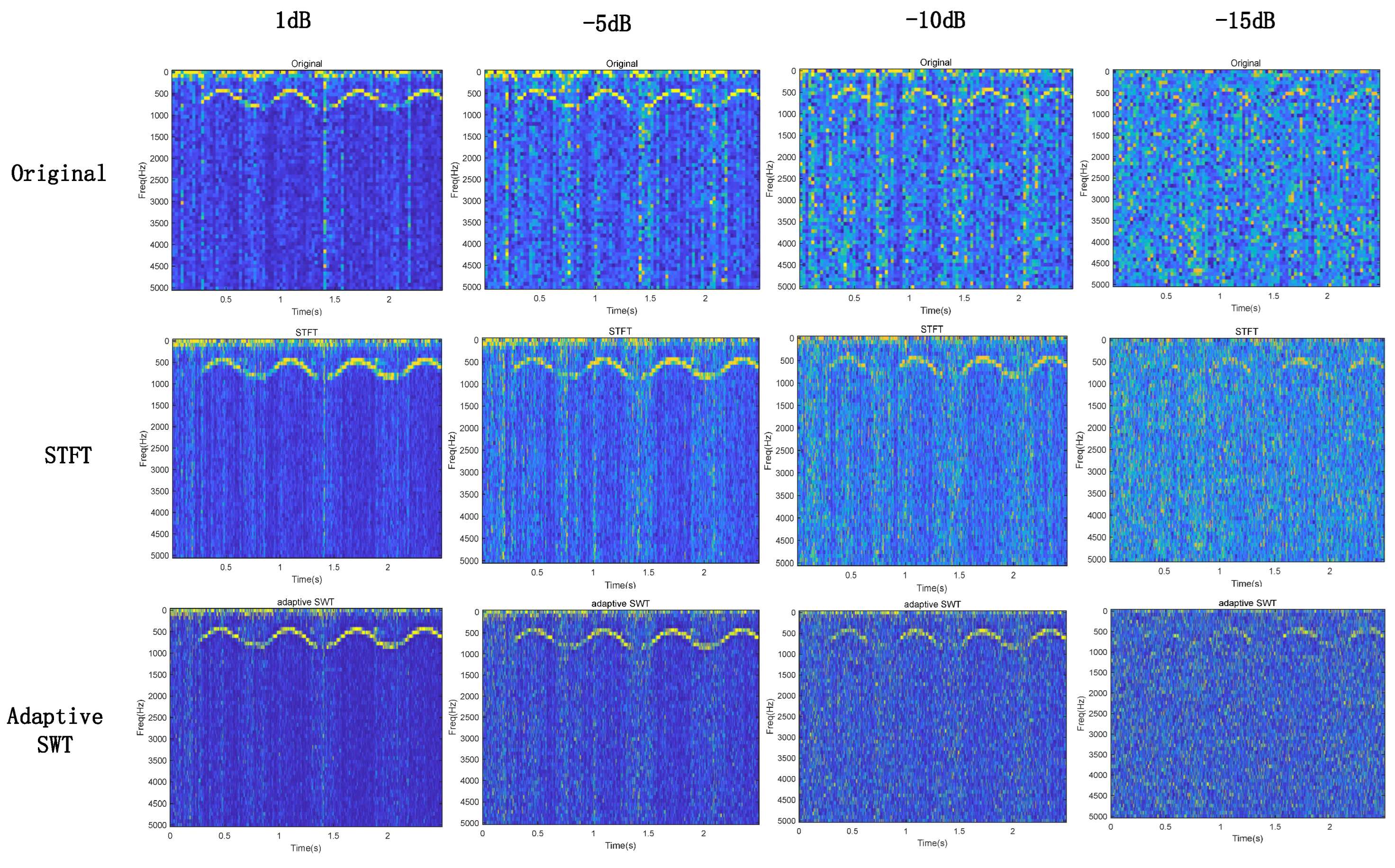
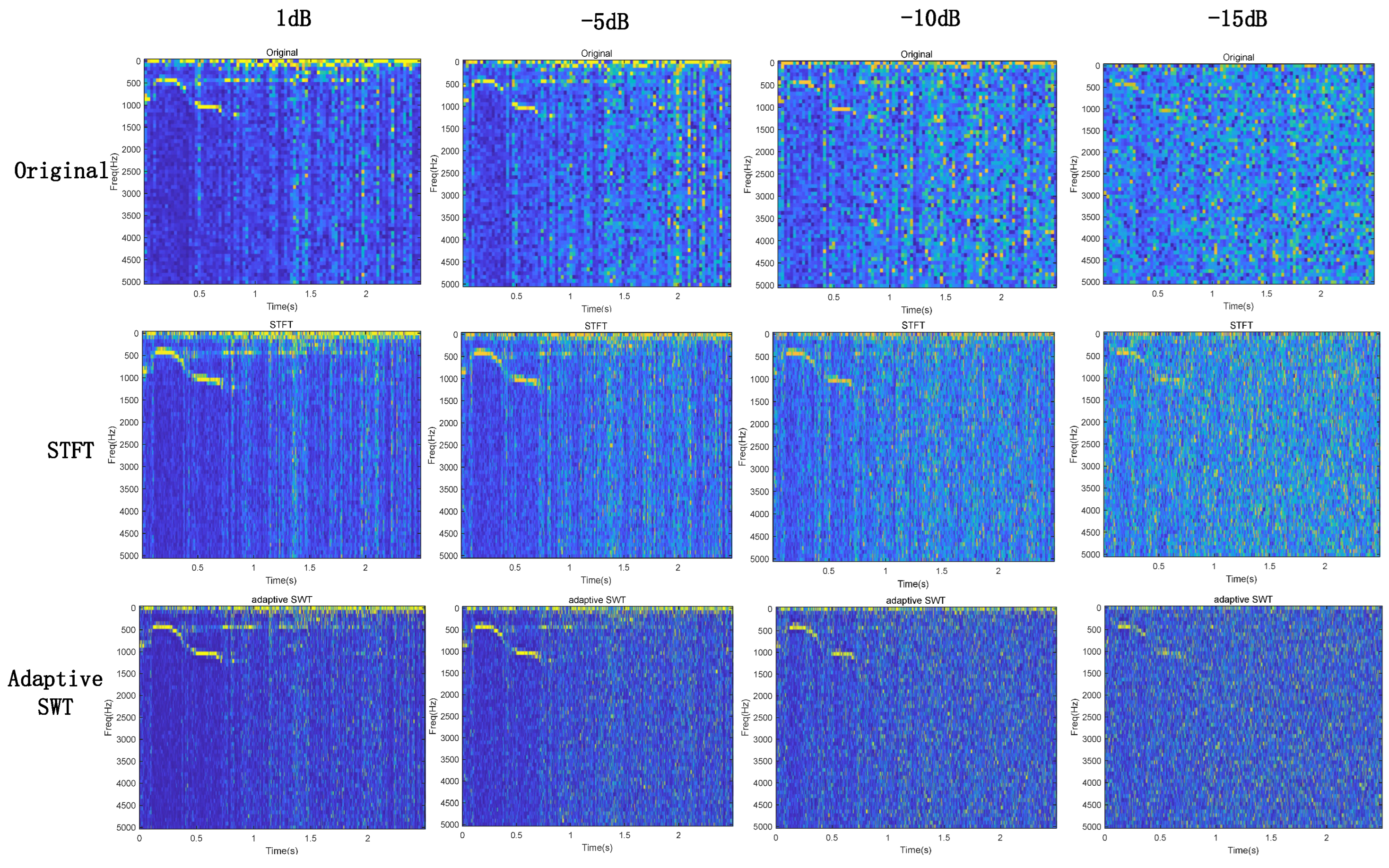
3.2.1. Comparative Experiment Based on the STFT, Fixed Parameter SWT and Adaptive SWT

In this part, we compared the performance of STFT with fixed parameter SWT and adaptive SWT. The Morlet wavelet parameter $\mu =1$, scale factor $a$ is discretized as $a_j=2^{j/n_v}\mathsf{\Delta }\mathrm{t}$, so, $n_v=32, j=\mathrm{1,2},\cdots n_v{\log }_{2}N.$ The time sliding window width of STFT is set to 1/10 of the signal length; fixed parameter $\sigma =6$ and ${\sigma }_{est}\left(t\right)$ is obtained according to the time-varying parameter estimation method based on the local Rényi entropy above. For the stationary and nonstationary parts of the bowhead whale whistle signal, the time-frequency diagram obtained by using the SWT with the time-varying parameter ${\sigma }_{est}\left(t\right),$ fixed parameter SWT and the standard STFT are shown in Figure 6.

Figure 6 makes it evident that the time-frequency aggregation of SWT is better than STFT, in which the adaptive SWT under the time-varying parameter ${\sigma }_{est}\left(t\right)$ is superior to fixed parameter SWT, regardless of whether it is the stationary or the nonstationary part of the whistle signal. Furthermore, the adaptive SWT time-frequency diagram’s background noise is reduced, which shows that the SWT transform under the time-varying parameter ${\sigma }_{est}\left(t\right)$ possesses a certain level of noise suppression capability. The calculated statistics of SCR for 10 segments of bowhead whale whistle and nonwhistle signals are as follows. For the bowhead whale stationary whistle, the SCRs obtained using the STFT were 189.423, 193.371, 184.242, 202.374, 194.923, 199.813, 191.432, 188.847, 194.455 and 183.470, respectively, and the SCRs obtained using the fixed parameter SWT were 272.846, 285.426, 286.357, 269.436, 278.476, 289.426, 263.356, 264.484, 273.462 and 265.051; the SCRs obtained using the adaptive SWT were 357.653, 368.354, 365.101, 363.467, 364.127, 366.203, 355.116, 361.674, 352.327 and 363.918. For the nonstationary whistle of bowhead whales, the SCRs obtained using the STFT were 183.948, 191.753, 186.203, 196.217, 2.03632, 191.756, 192.842, 189.523, 187.523 and 190.243, respectively. The SCRs obtained using the fixed-parameter SWT were 258.425, 263.272, 268.253, 267.246, 274.193, 262.226, 275.211, 268.165, 254.246 and 265.253; the SCRs obtained by adaptive SWT are 348.363, 352.625, 356.853, 347.260, 354.288, 355.232, 356.736, 356.462, 355.385 and 351.678, respectively. We calculated the average increase in SCR and the average percentage increase in SCR for 10 randomly selected stationary and nonstationary whistles described above to quantify the improvement in feature extraction.

Table 7. Comparison of improvement results of STFT, SWT and adaptive SWT on SCR.

	SCR of STFT	SCR of SWT	SCR of Adaptive SWT	Increasement (STFT-Adaptive SWT)	Percentage Increase (STFT-Adaptive SWT)
Stationary	192.235	274.832	361.794	169.559	88.20%
Nonstationary	191.364	265.649	353.508	162.144	84.37%

shows the bowhead whale SCR obtained by STFT, SWT and adaptive SWT. It is shows that the SCR achieved using the adaptive SWT was superior to that obtained using the fixed parameter SWT and STFT, regardless of whether it is the stationary or nonstationary section of the bowhead whale whistle. Among them, the SCR of the stationary and nonstationary part of the bowhead whale whistle based on the adaptive SWT was improved by 88.20% and 92.05%, respectively, compared to the STFT.

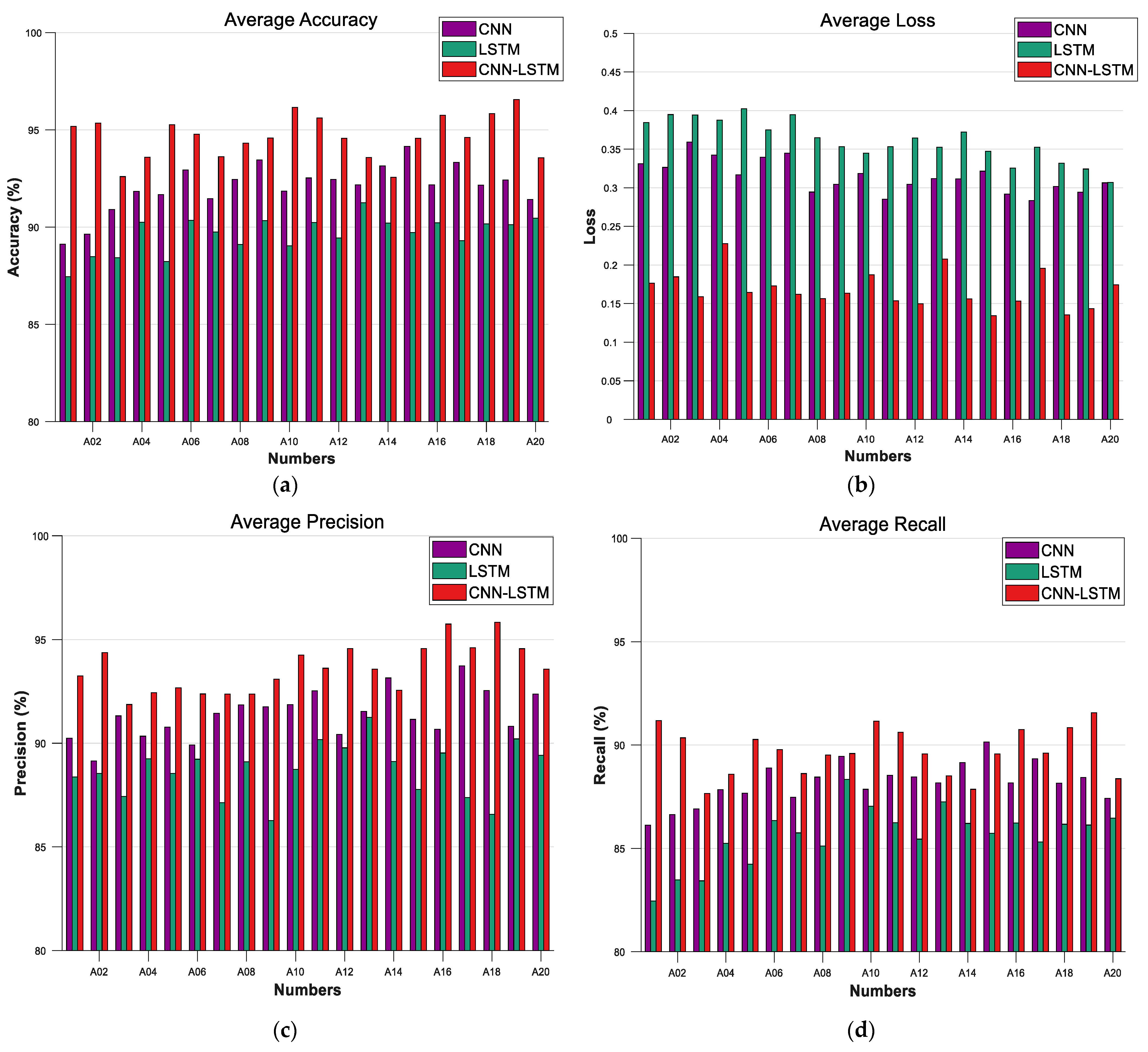
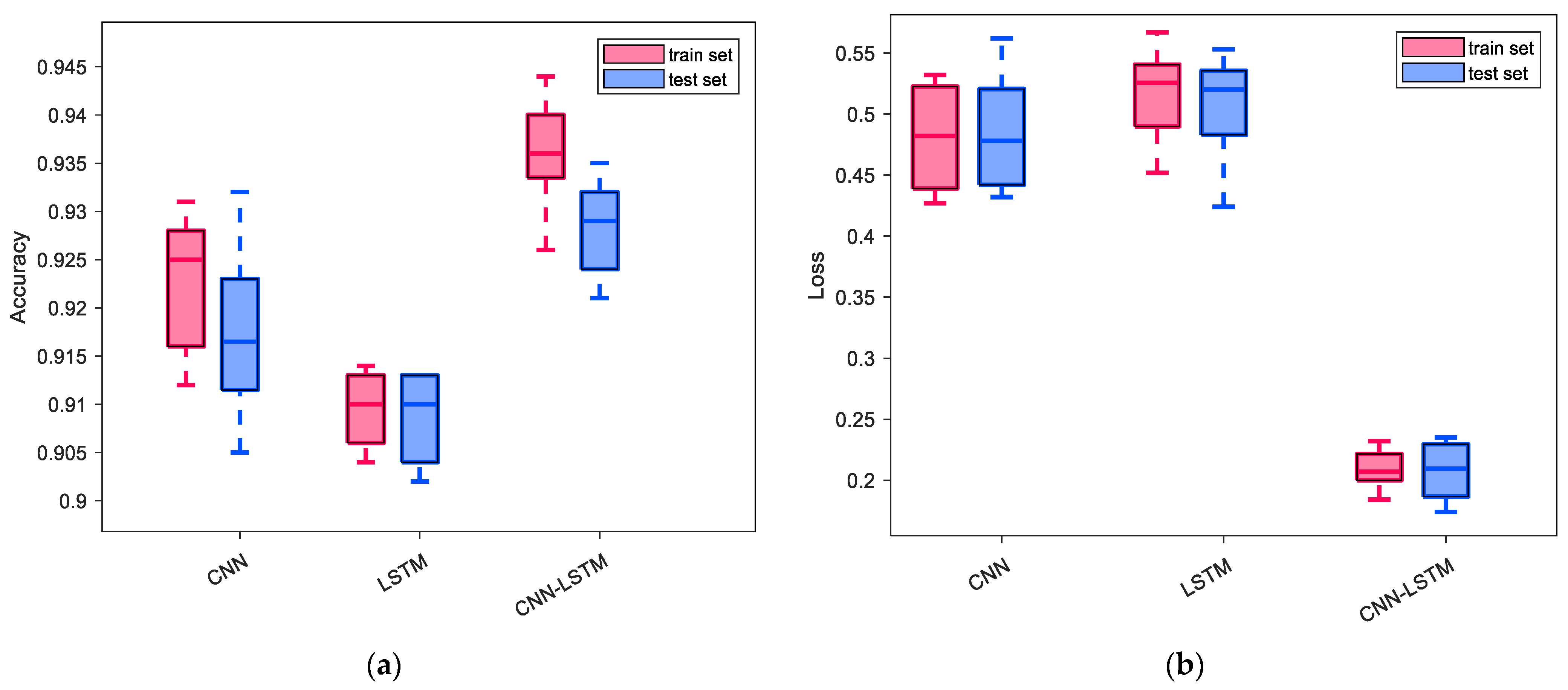
3.2.2. Comparative Experiment Based on the CNN, LSTM and CNN-LSTM

The SWT time-frequency diagram based on the Rényi entropy mentioned above is used as the feature input for the three models of CNN, LSTM and CNN-LSTM. Each model is trained 20 times to produce 20 networks and the test data are fed into the three models’ trained networks. Figure 7 shows the distribution of recognition accuracies and loss values for the train and test sets.

During the training phase, the accuracies of the three models on the test set gradually increased and stabilized, while the loss values gradually decreased and stabilized. Figure 8 demonstrates that the CNN-LSTM model outperforms the CNN and LSTM models in terms of accuracy and loss in the train and test set. Among them, the CNN-LSTM model’s average accuracy in the test set reached 92.82% and the average loss value in the test set was 0.22. These results suggest that the CNN-LSTM model presented in this study exhibits notable recognition and generalization capabilities.

3.2.3. Sensitivity Analysis

Figure 8 and Figure 9 show a comparison of the adaptive SWT, STFT and raw time-frequency plots of the stationary and nonstationary whistle signal of bowhead whales with noise at signal-to-noise ratios of 1 dB, −5 dB, −10 dB and −15 dB added, respectively.

Figure 8 and Figure 9 demonstrate that at a signal-to-noise ratio of −10 dB, the aggregation of adaptive SWT outperforms that of STFT. However, when the signal-to-noise ratio is −15 dB, the time-frequency aggregation benefit of adaptive SWT is diminished. The results in

Table 8. Rényi entropy results for stationary whistling in bowhead whales.

	1 dB	−5 dB	−10 dB	−15 dB
Original	4.123	6.779	7.548	8.413
STFT	3.521	5.345	6.533	7.817
Adaptive SWT	2.557	4.581	5.954	7.234

and

Table 9. Rényi entropy results for nonstationary whistling in bowhead whales.

	1 dB	−5 dB	−10 dB	−15 dB
Original	4.314	6.865	8.212	9.023
STFT	3.568	5.421	7.124	8.224
Adaptive SWT	2.685	4.612	6.296	7.752

explain this. As shown in Table 8 and Table 9, as the signal-to-noise ratio increases, the Rényi entropy value of STFT drops over the Rényi entropy value multiple of adaptive SWT.

Overall, adaptive SWT gives better time-frequency aggregation at various signal-to-noise ratios; however, when the signal-to-noise ratio is too high, the advantage of the method in this paper is decreased, which also presents new ideas for our future research.

3.2.4. Cross Validation

The data used for cross-validation of this paper came from the 60 sound recording files of bowhead whales from the Bering Strait of Barrow, Alaska, in the Watkins library mentioned above and 184 sound clips recorded over three consecutive winters in the Fram Strait in the DRYAD database. In total, approximately 24 min of recorded data were acquired. Through the framing operation, a total of 576 pieces of data were obtained. The data set is randomly divided into 10 sample sets with similar sample numbers, of which 4 sample sets have one less data. Nine sample sets are selected for training at a time, and the one remaining sample set is used as the validation set. The recognition results of each time are counted.

Figure 10 shows the line graph of the ten-fold cross-validation used in this paper. Horizontal coordinates represent the number of experiments and vertical coordinates represent the recognition accuracy of the corresponding experiments. The blue folds in the graph represent the changes in the recognition accuracy of the ten classifications under the ten experiments and the values of their corresponding classification recognition accuracies are 92.85%, 92.89%, 92.87%, 92.84%, 92.80%, 92.82%, 92.88%, 92.85%, 92.84% and 92.87%. The red horizontal line indicates the average change in the recognition accuracy of the ten experiments with an average accuracy of 92.85%. Therefore, the CNN-LSTM model in this paper obtains high recognition accuracy and has some stability.

4. Application

4.1. Comparative Experiments Based on Measured Data

We apply the frozen models and methods of this paper to the measured data in the Beaufort Sea. The measured data are derived from PAM, using a fixed autonomous recording device (AUSOMS ver. 3.5; Aqua-Sound Inc., Kobe, Japan). The location of the test site is approximately 72°29′24″N, 64°29′W (Nrs_01_2014-2015) and 72°29′26″N, 64°29′W (Nrs_01_2015-2017). In this phase, the test selects the two pieces of data of 131214_000000_AU_BS04 and 140311_060000_AU_BS04. Each piece of data is 20 min long, corresponding to 14 December 2014 and 9 June 2016.

We input the datasets 131214_000000_AU_BS04 and 140311_060000_AU_BS04 into 20 networks of 3 training models, respectively, then average the recognition results of the four measured records to achieve the final recognition result, as shown in Figure 11.

Analyzing the results in Figure 12, we can see that the LSTM model has the worst effect, the lowest overall recognition accuracy, the largest average loss and weak generalization ability. Its average recognition accuracy, recognition recall and recognition accuracy are all below 90%. Due to the powerful spatial feature extraction capability of the CNN model, it has a certain enhancement in accuracy compared to the LSTM model but the loss value after the model converges is still large. The CNN-LSTM model integrates the powerful spatial feature extraction capability of CNN and the advantages of LSTM in processing temporal information. The overall recognition accuracy rate reached 94.63%, the precision rate reached 93.61%, the recall rate reached 89.70% and the loss value was lower than that of CNN and LSTM.

In general, the CNN-LSTM model developed by linking CNN and LSTM may combine the advantages of CNN and LSTM, significantly increase model performance and improve whale call recognition accuracy. Moreover, the measured recording recognition results confirmed the anti-interference capability of this paper’s CNN-LSTM model.

4.2. Comparative Experiments with Published Articles

The linear discriminant analysis (LDA) and K Nearest Neighbors (KNN) model algorithms in Yang Wei et al.’s paper has a classification recognition accuracy of 100% [47]. In order to compare the KNN model and the CNN-LSTM model in this paper, we will replace the CNN-LSTM model under the algorithm of this paper with LDA and KNN models. Following the experiments, the classification recognition accuracies of LDA and KNN are 85.39% and 87.64%, respectively. In other words, the classification recognition accuracies of LDA and KNN are 7.46% and 5.21% lower than that of the CNN-LSTM model (92.85%) under the same measured data of this paper, respectively. This indicates that the CNN-LSTM model in this paper is better than LDA and KNN. To prove the effectiveness of the model algorithm in this paper, under the same data, we compare the recognition results of the algorithm in this paper with the LDA algorithm and KNN algorithm, respectively, and the results of the comparison are shown in Figure 12. This further illustrates the robustness of the methodology in this paper.

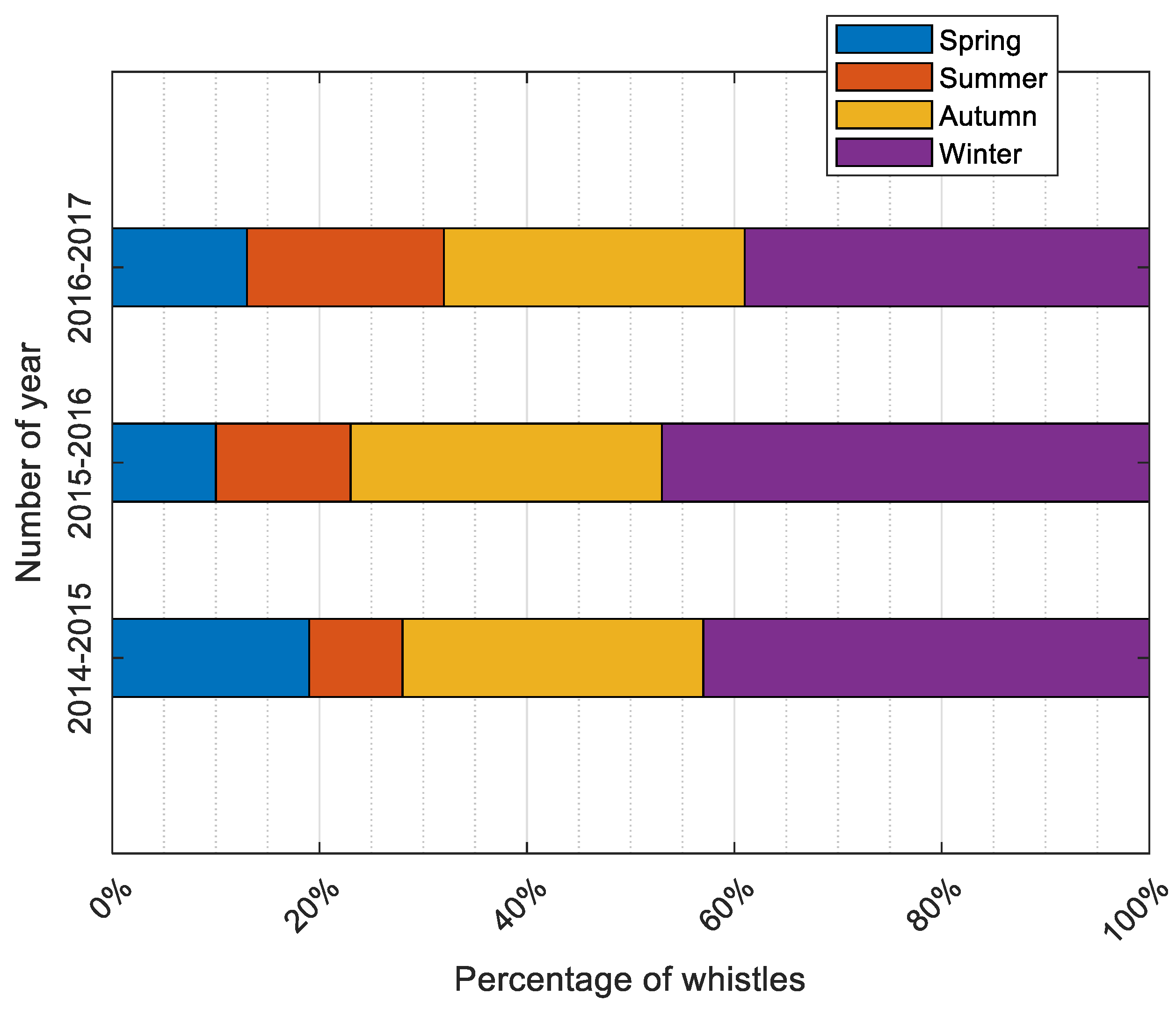
4.3. Comparative Experiments Based on Fisheries Ecology Studies

We use the method of this paper to recognize the bowhead whale whistles in the Beaufort Sea from 2014 to 2017. Our fundamental assumption is that the bigger the number of recognized voices, the greater the number of vocalizing bowhead whales. The seasonality of detected voices by the site is based on the Northern Hemisphere seasons. The seasons definity is according to Forney, KA et al. [48]. Specifically, spring (May, June), summer (July, August, September, October, November), autumn (December, January) and winter (February, March, April).

At the above sites, most of the bowhead whale whistles were detected during winter (Nrs_01_2014-2015: 64%, Nrs_01_2015-2017: 51%) or during autumn (Nrs_01_2014-2015: 33%, Nrs_01_2015-2017: 35%). We can obtain bowhead whales’ main seasonal movement characteristics and activity patterns in the Beaufort Sea by analyzing the recognition results, as shown in Figure 13.

Autumn and winter are peak seasons for bowhead whale voices in the Beaufort Sea, as shown in Figure 13. According to S.J. Insley et al. [48], they detected bowhead whales in 46 of the 4929 documents recorded in the northwestern Arctic, 12 of which were in the October–December period and 34 in the January 1–April 15 period. This result suggests that in Arctic waters, bowhead whales vocalize more frequently during the fall and winter months, which is generally consistent with the experimental results in this paper. Of course, we are only making broad trend-consistent comparisons. Bowhead whale vocalizations in the northwestern Arctic are concentrated in the autumn and winter because the endemic bowhead whale population in Arctic waters migrates southward to the Bering Strait for the winter in the autumn of each year and they migrate between the Bering and Beaufort Seas each year [49]. As a result, bowhead whales whistle more frequently from December to late February, including autumn (southbound) and spring (northbound) migrations. This migration is associated with changes in sea ice [50] and bowhead whales are adapted to marine environments dominated by sea ice. Moreover, Hannay et al. have shown that the timing of the autumn migration of bowhead whales is related to sea surface temperature and sea ice concentration [51]. Bowhead whales encounter a variety of ambient noises each year when they migrate from the Beaufort Sea to the Chukchi Sea into the Bering Strait and back. The majority of this ambient noise is caused by storms and ship traffic. The method used in this paper achieved better results even in this noise-inclusive situation, which further illustrates the effectiveness of this paper’s method.

5. Discussion

Based on a detailed introduction to the theory of synchronous compression continuous wavelet transform (SWT), this paper introduces a time-varying parameter based on the Rayleigh entropy to solve the problem that the continuous wavelet transform with a fixed wavelet parameter cannot optimize time-frequency aggregation in both the low-frequency and high-frequency bands at the same time. The experimental results suggest that the adaptive SWT presented in this work has significant advantages and stability. However, it should be emphasized that the frequency of bowhead whale whistles does not change much and low-order SWT can be used to obtain better results; we find it is limited to signals with slower instantaneous frequency changes. This is consistent with the research conclusions of J. Shi [52] and Xiang-Li Wang et al. [53]. For fast time-varying signals, the first-order frequency rate of change cannot be ignored; otherwise, there is a gradual increase in the frequency estimation error and the time-frequency aggregation will be reduced when dealing with signals with fast frequency changes. In this situation, an expanded high order synchrosqueezing transform and second order synchronous compression based on more precise instantaneous frequency estimation are needed. Higher resolution and more concentrated time-frequency energy aggregation are features of high order synchrosqueezing. Therefore, in future research, we will extend the synchrosqueezing transform to a higher order and make further theoretical analysis and derivation of the adaptive high order synchrosqueezing transform to meet the needs of signals with rapidly changing frequencies in practical work.

In terms of deep learning, in this paper, CNN and LSTM are connected to construct a deep learning model, i.e., the features extracted by the CNN model are then extracted by the LSTM model to obtain the final features. We should note that this method disrupts part of the time series characteristics of the data and loses part of the timing information of the original data, and then the use of LSTM to extract the features of the data will result in the LSTM not being able to utilize better all the information of the original data and the complete timing characteristics. Therefore, in future research, we will consider the concatenation of CNN and LSTM, that is, the weighted fusion of the features extracted by CNN and LSTM as the final features, to improve the recognition accuracy of the model.

In future research on bowhead whale sound recognition, these methods can be drawn upon to solve the problems of insufficient time-frequency features and poor contextualization in traditional whale sound recognition methods. This will provide technical support for future investigations of the distribution of bowhead whale populations and conservation of bowhead whales. Furthermore, the methods of this article could be combined with bottom exploration sonar technology to further advance the field of marine research’s remote sensing of oceanic rises.

6. Conclusions

This paper employs acoustic remote sensing technology to recognize bowhead whales, extracting bowhead whale voice features using adaptive SWT and recognizing bowhead whales using CNN-LSTM. The features of the bowhead whale whistle extracted using adaptive SWT were improved and their time-frequency aggregation was enhanced. The performance of STFT, SWT and adaptive SWT was compared by calculating the average SCR. When comparing the adaptive SWT to the STFT, the SCR of the stationary and nonstationary parts of the bowhead whale whistle improved by 88.20% and 92.05%, respectively. The average recognition performance of the CNN, LSTM and CNN-LSTM neural network models was evaluated using the same test set of measured recordings. The experimental results showed that the CNN-LSTM model recognition effect based on adaptive SWT is superior. The ten-fold cross-validation achieved an average recognition accuracy of 92.85%. The SCR of the stationary and the nonstationary parts of the bowhead whale whistle based on the adaptive SWT increased by 87.34% and 79.58%, respectively, compared to the STFT. This paper’s model’s average recognition accuracy rate of the measured recordings in the Beaufort Sea reached 94.63%, the precision rate reached 93.61% and the recall rate reached 89.70%. In the case of the same measured recording, the recognition model in this paper improves the accuracy by 7.46% and 5.21% compared to the methods LDA and KNN in the published articles, respectively. The experimental results also demonstrated the inter-annual pattern of change in the migratory characteristics of bowhead whales in the Beaufort Sea, with them vocalizing more in the autumn and winter, consistent with fisheries ecology research This further supports the model’s anti-interference and generalization abilities demonstrated in this work.

References

1. Moore, S.E. Marine mammals as ecosystem sentinels. J. Mammal. 2008, 89, 534–540. [Google Scholar] [CrossRef]
2. Laidre, K.L.; Peter Heide-Jørgensen, M.; Gissel Nielsen, T. Role of the bowhead whale as a predator in West Greenland. Mar. Ecol. Prog. Ser. 2007, 346, 285–297. [Google Scholar] [CrossRef]
3. Reeves, R.; Rosa, C.; George, J.C.; Sheffield, G.; Moore, M. Implications of Arctic industrial growth and strategies to mitigate future vessel and fishing gear impacts on bowhead whales. Mar. Policy 2012, 36, 454–462. [Google Scholar] [CrossRef]
4. George, J.C.; Zeh, J.; Suydam, R.; Clark, C. Abundance and Population Trend (1978–2001) of Western Arctic Bowhead Whales Surveyed Near Barrow, Alaska. Mar. Mammal. Sci. 2004, 20, 755–773. [Google Scholar] [CrossRef]
5. Jones, N. The Quest for Quieter Seas. Nature 2019, 568, 158–161. [Google Scholar] [CrossRef] [PubMed]
6. Kaklamanis, E.; Purnima, R.C.N.M. Optimal Automatic Wide-Area Discrimination of Fish Shoals from Seafloor Geology with Multi-Spectral Ocean Acoustic Waveguide Remote Sensing in the Gulf of Maine. Remote Sens. 2023, 15, 437. [Google Scholar]
7. Duane, D.; Godø, O.R.; Makris, N.C. Quantification of Wide-Area Norwegian Spring-Spawning Herring Population Density with Ocean Acoustic Waveguide Remote Sensing (OAWRS). Remote Sens. 2021, 13, 4546. [Google Scholar] [CrossRef]
8. Godin, O.A.; Katsnelson, B.G.; Qin, J.; Brown, M.G.; Zabotin, N.A. Application of time reversal to passive acoustic remote sensing of the ocean. Acoust. Phys. 2017, 63, 309–320. [Google Scholar] [CrossRef]
9. Zhu, C.; Garcia, H.; Kaplan, A.; Schinault, M.; Handegard, N.; Godø, O.; Ratilal, P. Detection, Localization and Classification of Multiple Mechanized Ocean Vessels over Continental-Shelf Scale Regions with Passive Ocean Acoustic Waveguide Remote Sensing. Remote Sens. 2018, 10, 1699. [Google Scholar] [CrossRef]
10. Churnside, J.H.; Naugolnykh, K.; Marchbanks, R.D. Optical remote sensing of sound in the ocean. In Proceedings of the SPIE 9111, Ocean Sensing and Monitoring VI, 91110T; SPIE: New York, NY, USA, 2014. [Google Scholar] [CrossRef]
11. Akulichev, V.A.; Bezotvetnykh, V.V.; Burenin, A.V.; Voytenko, E.A.; Kamenev, S.I.; Morgunov, Y.N.; Polovinka, Y.A.; Strobykin, D.S. Remote acoustic sensing methods for studies in oceanology. Ocean Sci. J. 2006, 41, 105–111. [Google Scholar] [CrossRef]
12. Burtenshaw, J.C.; Oleson, E.M.; Hildebrand, J.A.; McDonald, M.A.; Andrew, R.K.; Howe, B.M.; Mercer, J.A. Acoustic and satellite remote sensing of blue whale seasonality and habitat in the Northeast Pacific. Deep Sea Res. Part II Top. Stud. Oceanogr. 2004, 51, 967–986. [Google Scholar] [CrossRef]
13. Fretwell, P.T.; Jackson, J.A.; Ulloa Encina, M.J.; Häussermann, V.; Perez Alvarez, M.J.; Olavarría, C.; Gutstein, C.S. Using remote sensing to detect whale strandings in remote areas: The case of sei whales mass mortality in Chilean Patagonia. PLoS ONE 2019, 14, e0222498. [Google Scholar] [CrossRef]
14. Garcia, H.A.; Couture, T.; Galor, A.; Topple, J.M.; Huang, W.; Tiwari, D.; Ratilal, P. Comparing Performances of Five Distinct Automatic Classifiers for Fin Whale Vocalizations in Beamformed Spectrograms of Coherent Hydrophone Array. Remote Sens. 2020, 12, 326. [Google Scholar] [CrossRef]
15. Balcazar, N.E.; Tripovich, J.S.; Klinck, H.; Nieukirk, S.L.; Mellinger, D.K.; Dziak, R.P.; Rogers, T.L. Calls reveal population structure of blue whales across the southeast Indian Ocean and the southwest Pacific Ocean. J. Mammal. 2015, 96, 1184–1193. [Google Scholar] [CrossRef]
16. Chapman, R. A Review of “Passive Acoustic Monitoring of Cetaceans. Trans. Am. Fish. Soc. 2013, 142, 578–579. [Google Scholar] [CrossRef]
17. Campos-Cerqueira, M.; Aide, T.M. Improving distribution data of threatened species by combining acoustic monitoring and occupancy modelling. Methods Ecol. Evol. 2016, 7, 1340–1348. [Google Scholar] [CrossRef]
18. Tervo, O.M.; Christoffersen, M.F.; Parks, S.E.; Møbjerg Kristensen, R.; Teglberg Madsen, P. Evidence for simultaneous sound production in the bowhead whale (Balaena mysticetus). J. Acoust. Soc. Am. 2011, 130, 2257–2262. [Google Scholar] [CrossRef] [PubMed]
19. Ou, H.; Au, W.W.L.; Oswald, J.N. A non-spectrogram-correlation method of automatically detecting minke whale boings. J. Acoust. Soc. Am. 2012, 132, EL317–EL322. [Google Scholar] [CrossRef]
20. Gómez Blas, N.; de Mingo López, L.F.; Arteta Albert, A.; Martínez Llamas, J. Image Classification with Convolutional Neural Networks Using Gulf of Maine Humpback Whale Catalog. Electronics 2020, 9, 731. [Google Scholar] [CrossRef]
21. Xie, Z.; Zhou, Y. The Study on Classification for Marine Mammal Based on Time-Frequency Perception. In Proceedings of the 4th International Conference on Bioinformatics and Biomedical Engineering, Chengdu, China, 18–20 June 2010. [Google Scholar] [CrossRef]
22. Yuanfeng, M.; Chen, K. A time-frequency perceptual feature for classification of marine mammal sounds. In Proceedings of the 9th International Conference on Signal Processing, Beijing, China, 26–29 October 2008. [Google Scholar] [CrossRef]
23. Bahoura, M.; Simard, Y. Blue whale calls classification using short-time Fourier and wavelet packet transforms and artificial neural network. Digit. Signal Process. 2010, 20, 1256–1263. [Google Scholar] [CrossRef]
24. Jiang, B.L.; Duan, F.; Wang, X.; Liu, W.; Sun, Z.; Li, C. Whistle detection and classification for whales based on convolutional neural networks. Appl. Acoust. 2019, 150, 169–178. [Google Scholar] [CrossRef]
25. Ibrahim, A.K.; Zhuang, H.; Erdol, N.; Ali, A.M. A New Approach for North Atlantic Right Whale Upcall Detection. In Proceedings of the 2016 International Symposium on Computer, Consumer and Control (IS3C), Xi’an, China, 4–6 July 2016. [Google Scholar] [CrossRef]
26. Wang, Q.; Zhou, B.; Yu, W. Passive CFAR detection based on continuous wavelet transform of sound signals of marine animal. In Proceedings of the 2017 IEEE International Conference on Signal Processing, Communications and Computing (ICSPCC), Xiamen, China, 22–25 October 2017. [Google Scholar] [CrossRef]
27. Ou, H.; Au, W.W.L.; Van Parijs, S.; Oleson, E.M.; Rankin, S. Discrimination of frequency-modulated Baleen whale downsweep calls with overlapping frequencies. J. Acoust. Soc. Am. 2015, 137, 3024–3032. [Google Scholar] [CrossRef] [PubMed]
28. Adam, O. The use of the Hilbert-Huang transform to analyze transient signals emitted by sperm whales. Appl. Acoust. 2006, 67, 1134–1143. [Google Scholar] [CrossRef]
29. Daubechies, I.; Lu, J.; Wu, H.T. Synchrosqueezed wavelet transforms: An empirical mode decomposition-like tool. Appl. Comput. Harmon. Anal. 2011, 30, 243–261. [Google Scholar] [CrossRef]
30. Luo, X.; Chen, L.; Zhou, H.; Cao, H. A Survey of Underwater Acoustic Target Recognition Methods Based on Machine Learning. J. Mar. Sci. Eng. 2023, 11, 384. [Google Scholar] [CrossRef]
31. Hachicha Belghith, E.; Rioult, F.; Bouzidi, M. Acoustic Diversity Classification Using Machine Learning Techniques: Towards Automated Marine Big Data Analysis. Int. J. Artif. Intell. Tools 2020, 29, 2060011. [Google Scholar] [CrossRef]
32. Yang, H.; Lee, K.; Choo, Y.; Kim, K. Underwater Acoustic Research Trends with Machine Learning: General Background. J. Ocean. Eng. Technol. 2020, 34, 147–154. [Google Scholar] [CrossRef]
33. Mishachandar, B.; Vairamuthu, S. Diverse ocean noise classification using deep learning. Appl. Acoust. 2021, 181, 108141. [Google Scholar] [CrossRef]
34. Yang, H.; Li, J.; Shen, S.; Xu, G. A Deep Convolutional Neural Network Inspired by Auditory Perception for Underwater Acoustic Target Recognition. Sensors 2019, 19, 1104. [Google Scholar] [CrossRef]
35. Li, S.; Jin, X.; Yao, S.; Yang, S. Underwater Small Target Recognition Based on Convolutional Neural Network. In Proceedings of the Global Oceans 2020: Singapore–US Gulf Coast, Biloxi, MS, USA, 5–30 October 2020. [Google Scholar]
36. Miller, B.S.; Madhusudhana, S.; Aulich, M.G.; Kelly, N. Deep learning algorithm outperforms experienced human observer at detection of blue whale D-calls: A double-observer analysis. Remote Sens. 2022, 9, 104–116. [Google Scholar] [CrossRef]
37. Zhang, L.; Wang, D.; Bao, C.; Wang, Y.; Xu, K. Large-Scale Whale-Call Classification by Transfer Learning on Multi-Scale Waveforms and Time-Frequency Features. Appl. Sci. 2019, 9, 1020. [Google Scholar] [CrossRef]
38. Madhusudhana, S.; Shiu, Y.; Klinck, H.; Fleishman, E.; Liu, X.; Nosal, E.M.; Helble, T.; Cholewiak, D.; Gillespie, D.; Roch, M.A. Improve automatic detection of animal call sequences with temporal context. J. R. Soc. Interface 2021, 18, 20210297. [Google Scholar] [CrossRef]
39. Madhusudhana, S.; Shiu, Y.; Klinck, H.; Fleishman, E.; Liu, X.; Nosal, E.M.; Helble, T.; Cholewiak, D.; Gillespie, D.; Roch, M.A. Temporal context improves automatic recognition of call sequences in soundscape data. J. Acoust. Soc. Am. 2020, 148, 2442. [Google Scholar] [CrossRef]
40. Stafford, K.M.; Lydersen, C.; Wiig, Ø.; Kovacs, K.M. Data from: Extreme diversity in the songs of Spitsbergen’s bowhead whales. Biol. Lett. 2018, 14, 20180056. [Google Scholar] [CrossRef] [PubMed]
41. Erbs, F.; van der Schaar, M.; Weissenberger, J.; Zaugg, S.; André, M. Contribution to unravel variability in bowhead whale songs and better understand its ecological significance. Sci. Rep. 2021, 11, 168. [Google Scholar] [CrossRef] [PubMed]
42. Bu, L.R. Study on Identification and Classification Methods of Whale Acoustic Signals between Whale Species; Tianjin University: Tianjin, China, 2018. [Google Scholar] [CrossRef]
43. Daubechies, I. Ten Lectures on Wavelets; Society for Industrial and Applied Mathematics: Philadelphia, PA, USA, 1992. [Google Scholar]
44. Baraniuk, R.G.; Flandrin, P.; Janssen, A.J.E.M.; Michel, O.J.J. Measuring time-frequency information content using the Renyi entropies. IEEE Trans. Inf. Theory 2001, 47, 1391–1409. [Google Scholar] [CrossRef]
45. Stanković, L. A measure of some time–frequency distributions concentration. Signal Process. 2001, 81, 621–631. [Google Scholar] [CrossRef]
46. Zhao, J.; Mao, X.; Chen, L. Speech emotion recognition using deep 1D & 2D CNN LSTM networks. Biomed. Signal Process. Control 2019, 47, 312–323. [Google Scholar] [CrossRef]
47. Wei, Y. Research on Detection and Recognition Technology of Cetacean Call; Harbin Engineering University: Harbin, China, 2022. [Google Scholar] [CrossRef]
48. Forney, K.A.; Barlow, J. Seasonal Patterns in the Abundance and Distribution of California Cetaceans, 1991–1992. Mar. Mammal Sci. 1998, 14, 460–489. [Google Scholar] [CrossRef]
49. Insley, S.J.; Halliday, W.D.; Mouy, X.; Diogou, N. Bowhead whales overwinter in the Amundsen Gulf and Eastern Beaufort Sea. R. Soc. Open Sci. 2021, 8, 202268. [Google Scholar] [CrossRef] [PubMed]
50. Szesciorka, A.R.; Stafford, K.M. Sea ice directs changes in bowhead whale phenology through the Bering Strait. Mov. Ecol. 2023, 11, 8. [Google Scholar] [CrossRef] [PubMed]
51. Chambault, P.; Albertsen, C.M.; Patterson, T.A.; Hansen, R.G.; Tervo, O.; Laidre, K.L.; Heide-Jørgensen, M.P. Sea surface temperature predicts the movements of an Arctic cetacean: The bowhead whale. Sci. Rep. 2018, 8, 9658. [Google Scholar] [CrossRef]
52. Shi, J.; Chen, G.; Zhao, Y.; Tao, R. Synchrosqueezed Fractional Wavelet Transform: A New High-Resolution Time-Frequency Representation. IEEE Trans. Signal Process. 2023, 71, 264–278. [Google Scholar] [CrossRef]
53. Wang, X.-L.; Li, C.-L.; Yan, X. Nonstationary harmonic signal extraction from strong chaotic interference based on synchrosqueezed wavelet transform. Signal Image Video Process. 2018, 13, 397–403. [Google Scholar] [CrossRef]
Figure 1. Distribution ofPAM sites in the Beaufort Sea. Sites selected for this paper include Nrs_01_2014-2015 and Nrs_01_2015-2017.
Remotesensing 15 05346 g001
Figure 2. Diagrams of whale whistles from several species.
Remotesensing 15 05346 g002
Figure 3. The structure of the data preprocessing.
Remotesensing 15 05346 g003
Figure 4. Schematic diagram of the three steps.
Remotesensing 15 05346 g004
Figure 5. The structure of the CNN-LSTM neural network.
Remotesensing 15 05346 g005
Figure 6. Comparison of time-frequency diagrams of the whistle based on STFT, fixed parameter SWT and adaptive SWT. Yellow indicates bowhead whale whistles and blue indicates background voices. The red box shows an enlargement of one of the signals. (a1) Time-frequency diagram of bowhead whale’s stationary whistle based on STFT; (a2) time-frequency diagram of bowhead whale’s stationary whistle based on fixed parameter SWT; (a3) time-frequency diagram of bowhead whale’s stationary whistle based on adaptive SWT; (b1) time-frequency diagram of bowhead whale’s nonstationary whistle based on STFT; (b2) time-frequency diagram of bowhead whale’s nonstationary whistle based on fixed parameter SWT; (b3) time-frequency diagram of bowhead whale’s nonstationary whistle based on adaptive SWT.
Remotesensing 15 05346 g006
Figure 7. Boxplot distribution of the train and test set’s recognition accuracy and loss value. (a) Boxplot distribution of the train and test set’s recognition accuracy; (b) boxplot distribution of the train and test set’s loss.
Remotesensing 15 05346 g007
Figure 8. Comparison of bowhead whale stationary whistle signals added to various signal-to-noise ratios.
Remotesensing 15 05346 g008
Figure 9. Comparison of bowhead whale nonstationary whistle signals added to various signal-to-noise ratios.
Remotesensing 15 05346 g009
Figure 10. Ten-fold cross-validation diagram.
Remotesensing 15 05346 g010
Figure 11. Recognition results of measured recordings. (a) Statistical chart of the average accuracy of the measured recording recognition; (b) statistical chart of the average loss value of the measured recording recognition; (c) statistical chart of the average precision of the measured recording recognition; (d) statistical chart of the average recall of the measured recording recognition.
Remotesensing 15 05346 g011
Figure 12. Recognition accuracy of LDA, KNN and CNN-LSTM.
Remotesensing 15 05346 g012
Figure 13. Percentage of hours containing bowhead whale whistles each season.
Remotesensing 15 05346 g013