Study on the Impact of Offshore Wind Farms on Surrounding Water Environment in the Yangtze Estuary Based on Remote Sensing

Abstract

Offshore wind farms (OWFs), built extensively in recent years, induce changes in the surrounding water environment. The changes in the suspended sediment concentration (SSC) and chlorophyll-a concentration (Chl-aC) induced by an OWF in the Yangtze River Estuary were analyzed based on Chinese Gaofen (GF) satellite data. The results show the following: (1) The flow near the wind turbines makes the bottom water surge, driving the sediment to “re-suspend” and be lost, deepening the scour pit around the bottom of the wind turbines, which is known as “self-digging”. The interaction between the pillar of a wind turbine and tidal currents makes hydrodynamic factors more complicated. Blocking by wind turbines promoting the scour of the bottom seabed of the OWF results in speeding up the circulation rate of sediment loss and “re-suspension”, which contributes to the change in the SSC and Chl-aC. This kind of change in sediment transport in estuarine areas due to human construction affects the balance of the ecological environment. Long-term sediment loss around wind turbines also influences the safety of wind turbines. (2) The SSC and Chl-aC are mainly in the range of 200–600 mg/L and 3–7 μg/L, respectively, in the OWF area, higher than the values obtained in surrounding waters. The SSC and Chl-aC downstream of the OWF are higher than those upstream, with differences of 100–300 mg/L and 0.5–2 μg/L. High SSC and Chl-aC “tails” appear downstream of wind turbines, consistent with the direction of local tidal currents, with lengths in the range of 2–4 km. In addition, the water environment in the vicinity of a wind turbine array, with a roughly 2–5 km scope (within 4 km during flooding and around 2.5 km during ebbing approximately) downstream of the wind turbine array, is impacted by the OWF. (3) In order to solve the problem of “self-digging” induced by OWFs, it is suggested that the distance between two wind turbines should be controlled within 2–3.5 km in the main flow direction, promising that the second row of wind turbines will be placed on the suspended sediment deposition belt induced by the first row. In this way, the problems of ecosystem imbalance and tidal current structure change caused by sediment loss because of local scouring can be reduced. Furthermore, mutual compensation between wind turbines can solve the “self-digging” problem to a certain extent and ensure the safety of OWFs.

1. Introduction

Numerous human initiatives, including reclamation projects [1], sea-crossing bridges [2], port construction [3], offshore wind projects [4], and more, have been built in the coastal waters of various countries in recent years. The influence of these projects on the surrounding sea environment is complicated. On the one hand, it meets the needs of human development and takes full advantage of resources. On the other hand, the original environmental balance is inevitably disrupted, reflected in the following aspects: (1) changes in local marine ecosystems, as marine infrastructure can have substantial cumulative and negative impacts on water pollution, biodiversity decrease, and habitat loss [5,6,7,8,9]; (2) changes in the physical environment, as marine engineering can change some natural conditions such as coastlines, coastal topography, and the distribution of suspended sediment [10] in coastal waters, further affecting the offshore flow field [11,12,13]. Taking the Yangtze Estuary as an example, although it is a famous fishing field, the marine ecological environment of the Yangtze Estuary is generally in an unhealthy state due to the impact of human engineering [14,15,16].

Many methods have been applied to analyze the impacts of nearshore constructions on ocean environmental factors. Based on non-remote-sensing methods (tidal current, numerical simulation, etc.) and remote sensing methods, many researchers have studied the impact of human engineering on the offshore water environment. For instance, FVCOM [17] was used to simulate the changes in the hydrodynamic environment and suspended sediment (SS) transport in Meizhou Bay after reclamation engineering, further analyzing the reasons for the weakening of the water exchange capacity and the decrease in the bay self-purification capacity. Using the MIKE21 model, Chen [18] studied the changes in the characteristics of the flow field and SS diffusion around the Dafeng River Bridge and suggested that measures should be taken to reduce SS diffusion during construction. By simulating the scour and deposition of sediments before and after the construction of the Jiaozhou Bay cross-sea bridge, Zhang [19] found that the siltation increased on the north and south sides of the bridge pier, and the scour intensity increased on the east and west sides of the pier.

In addition, the sea surface temperature (SST) decreased and the SSC increased downstream of the bridge, as observed by HY-1C and Landsat-8 satellites [20]. Furthermore, based on GF-4 and HY-1C satellite data, the temporal and spatial changes in Chl-a and suspended matter in China’s coastal waters were analyzed [21], and it was indicated that both Chl-aC (Chl-a concentration) and SSC were higher downstream of Donghai Bridge as well as downstream of islands near the Yangtze River Estuary in comparison to the Chl-aC and SSC upstream. It was also revealed that the influence range of Chl-aC downstream of the bridge pier can reach 0.3–1.5 km away from the bridge. Some researchers have also applied remote sensing data to monitor oil spills on drilling platforms [22,23].

The influence of OWFs on the water environment has been studied by many researchers. Very long wakes induced by wind farms can be observed easily through SAR data [24]. Additionally, Lu [25] proposed that Chl-aC in the region of OWFs has obvious aggregation and enhanced spatial autocorrelation. Zhang [26] and Wang [27] held the same view on tidal current structure and emphasized that OWFs have little effect on the whole structure of tidal currents in the sea area, but that they rather mostly affect the surrounding area of wind turbines, based on a two-dimensional numerical model. Near the root of wind turbines, the current velocity increases, while the tidal current velocity surrounding the turbines decreases both at the facing waterside and the backwater side of the wind turbines.

Meanwhile, an increase in the temperature of the OWF area and a decrease in humidity were indicated by Siedersleben [28] based on the WRF model. In addition to the influence of OWFs on surrounding SSC, Chl-aC, temperature, and tidal current, many researchers have also analyzed the change in the living environment of the organisms around OWFs. Zhan [29], Song [30], and Wilber [31] revealed the effects of OWFs on benthic organisms from the aspects of community structure, habitat change, and spatial–temporal patterns. Furthermore, by studying benthic organisms in the OWF region of the North Sea, Coates [32] and Pollock [33] discovered that the OWF area could provide a foraging habitat and refuge, potentially boosting biodiversity. Studies [34] have shown that the structure of the fish community in the OWF area and adjacent waters of the Yangtze River Estuary is impacted by factors such as dissolved oxygen, temperature, depth, and salinity. However, the primary disturbance factors are associated with seasonal and environmental factors, and the wind farm exerts a limited influence on them. Due to the numerous studies demonstrating the potential of OWFs in increasing biodiversity and providing habitats for surrounding organisms, further research is being conducted to establish a theoretical framework for integrating offshore wind farms with marine ranching [35,36,37,38].

The small diameter and spacing of the individual wind turbines present a challenge for conventional low-resolution remote sensing satellite data, as they cannot provide the necessary spatial resolution to accurately monitor the impact of wind turbines on the water environment. Therefore, it is imperative to analyze SSC and Chl-aC based on high-resolution satellite data like GF-6 (PMS) to reveal the specific changes caused by both OWFs and individual wind turbines. The launch of the Chinese Gaofen (GF) satellite has brought about high-resolution satellite data with exceptional characteristics, including high resolution, wide coverage, high quality, and efficient imaging. Among satellites capable of achieving a spatial resolution scale of two meters, the Gaofen-6 satellite (GF-6) with its PMS sensor offers an impressive coverage scope of up to 95 km, allowing for detailed analysis of water environment changes around individual wind turbines.

High-spatial-resolution satellite images from the Chinese GF were applied to investigate the change in SSC and Chl-aC induced by an OWF in the surrounding sea area in the Yangtze Estuary. Specifically, this study focuses on the changes in water environmental factors in the OWF area and around individual wind turbines.

The novelty of this paper includes the following: (1) evaluating the impact of an existing OWF on the surrounding water environment; (2) proposing suggestions for the reasonable layout of wind turbines for future OWFs based on the analysis of the changes in ocean environmental factors induced by an existing OWF.

This paper takes the background of the Yangtze River Estuary, which is characterized by complicated tidal currents, freshwater injection, shallow water depth (gradually increasing from west to east), irregular semi-diurnal tide, high SS, and muddy bottom. This study holds a certain reference value for the assessment of environmental impacts caused by OWFs and the development and protection of the marine environment. Further research is needed to understand the changes in SSC and Chl-aC induced by OWFs under other environmental backgrounds.

2. Materials and Methods

2.1. Study Area

The Yangtze Estuary, originating from the Qinghai–Tibet Plateau [39] and connecting the Yangtze River basin and the East China Sea, is the largest estuary in China. Characterized by three bifurcation systems in the channel and four outlets into the sea, the estuary features a gradually broadening channel from west to east, presenting a trumpet shape. In the east, the Kuroshio Warm Current passes by; in the north, the central Jiangsu coastal water and the Yellow River Cold Water Mass flow southward; the Taiwan Warm Current moves north. Along the coast, rich nutrients and salts are found in the Zhoushan Islands (Figure 1a) [40]. The Yangtze River Estuary is a moderately strong tidal estuary and an irregular semi-diurnal tide estuary, carrying a large amount of SS into the sea [40]. Influenced by maritime and continental climate, the region experiences warm and humid conditions [41], with southerly winds in summer and northerly winds in winter. Generally, the sea surface temperature ranges between 5 and 30 °C [42], and the surface salinity increases from west to east, exhibiting seasonal characteristics [43].

The Lingang OWF consists of 53 wind turbines, arranged roughly parallel from northeast to southwest, forming an irregular polygon (Figure 1e). Taking the northwest to southeast direction as the base direction (oblique direction), the distance between adjacent wind turbines is about 1.5–1.8 km, while the spacing of each row ranges from 2 to 2.5 km. The spacing in the middle of the OWF is wider compared to the surrounding area. Additionally, the shortest distance of the OWF from the shore is approximately 10 km, with a water depth of about 5~8 m (Figure 1b) [44]. According to completion time, the site can be divided into two parts: the north and south sections. By the end of 2016, Phase II of the north side project had completed 25 wind turbines, while Phase I of the south side project had constructed 28 wind turbines by the end of 2018 (Figure 1e).

Located in the junction of the Yangtze Estuary and Hangzhou Bay, the Lingang OWF is primarily affected by the interaction effects of tidal currents (Figure 1b) [44]. The key features of the tidal current in this area include a longer duration of the ebb tide compared to the flood tide and a flow velocity that is larger during the flood tide and smaller during the ebb tide [44,45]. In addition, the OWF is positioned in the maximum turbidity zone of the estuary, where there is an abundance of suspended material and nutrients [45].

2.2. Satellite Data

The GF-1 satellite (launched on 26 April 2013) and GF-6 satellite (launched on 2 June 2018) were both launched using the Long March-2-D carrier rocket. The operational network of these two satellites has reduced the 4-day revisiting observation cycle of China’s land area to 2 days, significantly enhancing the scope and timeliness of remote sensing data acquisition. Particularly, the monitoring capacity for agriculture, forestry, and grassland resources has seen significant improvement. As a low-orbit optical remote sensing satellite, the GF-6 satellite is equipped with a 2 m panchromatic/8 m multispectral high-resolution camera (PMS) and a 16 m multispectral medium-resolution wide-format camera (WFV). Its PMS sensor boasts the largest width of up to 95 km among satellites with a two-meter resolution. Additionally, the GF-6 WFV camera has incorporated the “red edge” band and ultraviolet band based on the GF-1 WFV camera, which effectively reflects the specific spectral characteristics of crops. Furthermore, GF-6 is not only the first GF satellite to achieve precise agricultural observation in China [46] but also plays an important role in resource estimation [47] and fractional vegetation cover extraction [48].

In this study, GF-1 WFV, GF-6 WFV, and GF-6 PMS satellite images (2021–2022) were acquired from the China Centre for Resources Satellite Data and Application (https://data.cresda.cn/, accessed on 27 October 2022) to analyze the detail changes in SSC and Chl-aC near the OWF in the Yangtze River Estuary area. Further detailed information about the GF-1 and GF-6 WFV and PMS sensors is provided in

Table 1. Introduction of GF-6 WFV and PMS sensor parameters.

Orbital	Sensor	Band No.	Spectral Coverage (μm)	Spatial Resolution (m)	Imagery Width (km)
Sun-synchronous orbit	GF-6 WFV	Band 1	0.45–0.52	≤16.0	≥800
		Band 2	0.52–0.59
		Band 3	0.63–0.69
		Band 4	0.77–0.89
		Band 5	0.69–0.73
		Band 6	0.73–0.77
		Band 7	0.40–0.45
		Band 8	0.59–0.63
Sun-synchronous orbit	GF-6 PMS	Band 1	0.45–0.52	8	≥90
		Band 2	0.52–0.60
		Band 3	0.63–0.69	2
		Band 4	0.76–0.90
		Band 5	0.45–0.90

and

Table 2. Introduction of GF-1 WFV and PMS sensor parameters.

Orbital	Sensor	Band No.	Spectral Coverage (μm)	Spatial Resolution (m)	Imagery Width (km)
Sun-synchronous orbit	GF-1 WFV	Band 1	0.45–0.52	16	800
		Band 2	0.52–0.59
		Band 3	0.63–0.69
		Band 4	0.77–0.89
Sun-synchronous orbit	GF-1 PMS	Band 1	0.45–0.52	8	60
		Band 2	0.52–0.59
		Band 3	0.63–0.69	2
		Band 4	0.77–0.89
		Band 5 (PAN)	0.45–0.90

.

2.3. Wind Field, SST, SSS, Tidal Current, and Topography Data

Wind field data, SST (°C) data, sea surface salinity (SSS) (‰) data, tidal current data, and topography data were used to provide the background information of the OWF, encompassing topography, hydrodynamic conditions, and hydrological elements, in order to uncover the mechanism of the change in SSC and Chl-aC induced by the OWF. Detailed data resources and relevant information can be found in Table 3.

The wind field data were derived from the ERA-Interim (ECMWF Re-Analysis-Interim) dataset, which is one of several datasets generated by the ECMWF through a series of projects. ERA5 [49] is the fifth-generation ECMWF reanalysis covering the past 40 to 70 years of global climate and weather, providing hourly estimation data including wind, temperature, rainfall, snow and sea ice, waves, and land surface. Additionally, the finite volume coastal ocean model (FVCOM) [50] was utilized to simulate the tidal current information for eight time periods within a day in 2020. This model is designed to accurately represent complex coastline changes [51]. SST data were obtained from APDRC, which also offers wind speed, sea surface height, sea surface salinity, and other related data. SSS (‰) data were derived from global ocean physical analysis and prediction products. Furthermore, the National Marine Science Data Center provided a dataset of topographic information, collected from data published by various foreign organizations, encompassing global ocean and land grid elevation topographic data with resolutions ranging of 5′, 2′, 1′, 30′′, and 15″.

Table 3. Data sources and relevant information.

Field (Units)	Data Source	Spatiotemporal Scale	Reference
MODIS-SST (°C)	MODIS Aqua monthly 4 km	4 km/day	http://apdrc.soest.hawaii.edu/data/data.php/, accessed on 27 November 2022
SSS (‰)	GLOBAL_ANALYSIS_FORECAST_PHY_001_024	0.083°/1 month	https://data.marine.copernicus.eu/product/GLOBAL_ANALYSISFORECAST_PHY_001_024/description, accessed on 20 November 2022
10 m wind	ERA5 monthly averaged data	0.25°/1 month	https://www.ecmwf.int/, accessed on 27 November 2022
Ocean current (m/s)	FVCOM	1 km/1 h	[50]
Topography	Submarine Topography Dataset	5′/1	http://mds.nmdis.org.cn/, accessed on 20 November 2022

Table 3. Data sources and relevant information.

Field (Units)	Data Source	Spatiotemporal Scale	Reference
MODIS-SST (°C)	MODIS Aqua monthly 4 km	4 km/day	http://apdrc.soest.hawaii.edu/data/data.php/, accessed on 27 November 2022
SSS (‰)	GLOBAL_ANALYSIS_FORECAST_PHY_001_024	0.083°/1 month	https://data.marine.copernicus.eu/product/GLOBAL_ANALYSISFORECAST_PHY_001_024/description, accessed on 20 November 2022
10 m wind	ERA5 monthly averaged data	0.25°/1 month	https://www.ecmwf.int/, accessed on 27 November 2022
Ocean current (m/s)	FVCOM	1 km/1 h	[50]
Topography	Submarine Topography Dataset	5′/1	http://mds.nmdis.org.cn/, accessed on 20 November 2022

2.4. Data Processing

2.4.1. Data Preprocessing

The preprocessing of the GF-1 (WFV) and GF-6 (WFV and PMS) images comprised radiometric calibration, atmospheric correction, orthophoto correction, and image fusion [52]. Initially, the radiation calibration transformed the digital number (DN) value of the raw image into a radiance value using the following equation [53]:

$$L_{\lambda }=\mathrm{G}\mathrm{a}\mathrm{i}\mathrm{n}\ast \mathrm{D}\mathrm{N}+\mathrm{O}\mathrm{f}\mathrm{f}\mathrm{s}\mathrm{e}\mathrm{t}$$

(1)

where $L_{\lambda }$ is the spectral radiation, and Gain and Offset are the calibration coefficients. The unit is $\mathrm{W}\times {\mathrm{m}}^{-2}\times {\mathrm{s}\mathrm{r}}^{-1}\times {\mathrm{\mu }\mathrm{m}}^{-1}$. The Gain and Offset values for the GF-1 (WFV) and GF-6 (WFV and PMS) were obtained from the China Resources Satellite Application Center (http://www.cresda.com/, accessed on 9 October 2023), as shown in

Table 4. Radiometric calibration parameters of the GF satellite in 2021.

Sensor	Calibration Coefficients	PAN	Band 1	Band 2	Band 3	Band 4	Band 5	Band 6	Band 7	Band 8
GF-1 WFV1	Gain	-	0.1722	0.1496	0.1227	0.1308	-	-	-	-
	Offset	-	0	0	0	0	-	-	-	-
GF-6 WFV	Gain	-	0.0633	0.0532	0.0508	0.0325	0.0523	0.0463	0.0670	0.0591
	Offset	-	0	0	0	0	0	0	0	0
GF-6 PMS	Gain	0.0577	0.0821	0.0671	0.0518	0.0310	-	-	-	-
	Offset	0	0	0	0	0	-	-	-	-

.

Additionally, in order to eliminate atmospheric errors, the Fast Line-of-Sight Atmospheric Analysis of Spectral Hypercubes (FLAASH) method was employed to perform atmospheric correction on GF satellite data. This model converted the radiance to the land surface reflectance [54]. Furthermore, orthographical correction was carried out using the rational polynomial coefficient (RPC) information of the GF satellite. The corrections accounted for terrain effects and distortions caused by camera orientation, with GMTED2010 (The Global Multi-resolution Terrain Elevation Data 2010) data serving as a reference [55].

Regarding image fusion [52], we utilized the nearest-neighbor diffusion-based pan sharpening (NNDiffuse pan-sharpening) method developed by the Rochester Institute of Technology [56]. This involved merging panchromatic (2 m resolution) and multispectral (8 m resolution) images. The resulting image exhibited enhanced richness and accuracy, combining the advantages of multiple spectra and high spatial resolution (2 m). This facilitated subsequent analysis and research of GF-6 PMS images.

The software tools Envi 5.3 and Python 3.8 were employed to process all images.

2.4.2. SSC Inversion

The study area, situated at the Yangtze River Estuary, is known for its high turbidity. As a result, the chosen inversion model for this area should be suitable for regions with high SS. In this study, we employed Cai’s double-band linear model, as previously proposed [57] for SSC inversion using GF satellite data. This model is adept at detecting SSC in a high-SS environment:

$$SSC=314.435\ast R\_Red+3805.982\ast R\_NIR+28.54$$

(2)

Here, $R\_Red$ and $R\_NIR$ are the values in the red and near-infrared bands after atmospheric correction, respectively. SSC is in mg/L.

2.4.3. Inversion of Chlorophyll-a Concentration

In this study, we utilize the PMS-Chla-named model (Formula (3)) built by Tang in a previous study [58]. This model combines the green and red bands to estimate Chl-aC. It was specifically designed for the adjacent area of the Yangtze River Estuary, located on the south side of the estuary and the outer edge of Hangzhou Bay in the East China Sea. The water quality of this area is similar to that of the study area. Therefore, the PMS-Chla-named model (Formula (3)) is suitable for performing Chl-aC inversion in this study.

$$\begin{gathered} \mathrm{X}=\mathrm{R}\mathrm{r}\mathrm{s}\left(\mathrm{B}3\right)/\mathrm{R}\mathrm{r}\mathrm{s}\left(\mathrm{B}2\right) \\ \rho =\exp \left(1.401{\mathrm{X}}^{2.423}\right) \end{gathered}$$

(3)

Here, ρ represents the concentration of Chl-a in mg/L, and Rrs (B2) and Rrs (B3) are the remote sensing reflectance in the green and red bands of the PMS image data, respectively.

3. Results

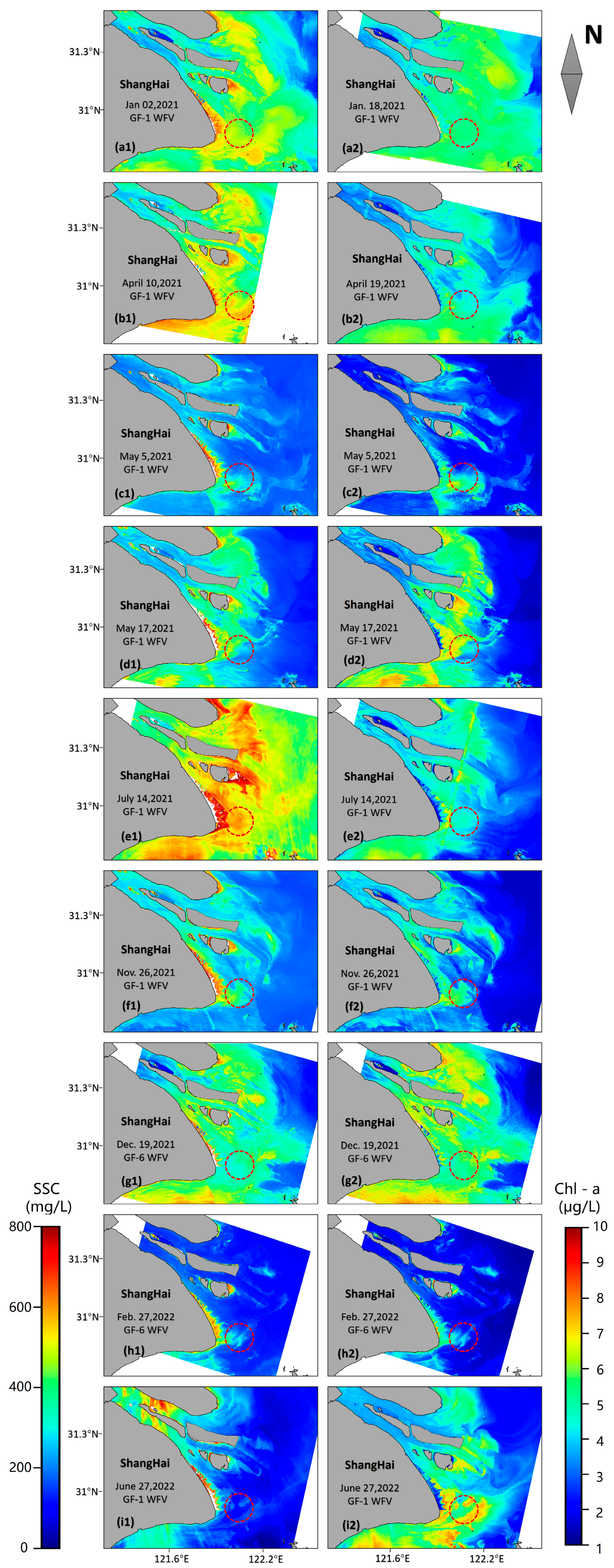
3.1. SSC and Chl-aC in the Yangtze River Estuary

Figure 2 illustrates the distribution of SSC and Chl-aC in the Yangtze Estuary for the period from January 2021 to June 2022. Generally, SSC and Chl-aC levels in the estuary are relatively high, in the ranges of 200–800 mg/L and 2–8 μg/L, respectively. Moreover, their distribution patterns are similar, with high values predominantly located near the coastline. Spatially, SSC and Chl-aC show a fan-shaped distribution, gradually increasing and then decreasing from the inner to the outer estuary, reaching approximately 200 mg/L and 2 μg/L, respectively.

The seasonal variation in SSC and Chl-aC is evident. In winter (Figure 2(a1,g1)), SSC levels are generally higher compared to those in summer (Figure 2(i1)). Conversely, Chl-aC exhibits higher levels in spring (Figure 2(b2,d2)) and summer (Figure 2(e2,i2)) than in autumn (Figure 2(f2)) and winter (Figure 2(h2)). However, it is worth noting that elevated SSC levels are also observed notably in July and August (Figure 2(e1)), ranging between 300 and 800 mg/L. In some areas near the coastline, the highest recorded SSC value exceeds 800 mg/L.

The concentration distribution characteristics of SS and Chl-aC are closely linked to ebb and flood tides in the estuary. During the ebb tide (tidal current flows from west to east), SSC (Figure 2(c1,h1)) and Chl-aC (Figure 2(b2,c2,h2)) remain relatively low in the channel in the inner estuary of the Yangtze River Estuary. However, during the flood tide, SSC (Figure 2(a1,b1,d1,e1,f1,g1,i1)) and Chl-aC (Figure 2(a2,d2,e2,f2,g2,i2)) levels rise. The area of maximum turbidity occurs in the outer estuary of the Yangtze Estuary, with SSC and Chl-aC gradually diminishing from west to east. There is also a noticeable high SSC aggregation area (Figure 2(b1,g1,i1)) during flood tide, as well as Chl-aC (Figure 2(d2,e2,g2)) in the southwest region of the Yangtze River Estuary near Hangzhou Bay. Additionally, SSC and Chl-aC downstream of the bridge, OWF, and islands are significantly higher than those upstream (Figure 2(c1,d1,c2,d2,f2)), regardless of whether it is a flooding or ebbing period.

3.2. SSC and Chl-aC near the OWF

Figure 3 provides a detailed view of the distribution of SSC and Chl-aC near the OWF. Generally, the SSC and Chl-aC in the waters around the OWF are in the ranges of 200–600 mg/L and 3–7 μg/L, respectively, which are significantly higher than those in the surrounding water, with differences of 100–300 mg/L and 1–3 μg/L, respectively. The “aggregation area” of high SSC (Figure 3c,g) and Chl-aC (Figure 3l,o) is predominantly located downstream of the OWF. During both flooding and ebbing tides, long high-concentration “tails” are observed downstream of the wind turbines (Figure 3c,e,f,h,l–n). Additionally, the settling distance of the suspended sediment increases with the tidal current velocity, regardless of flood tide or ebb tide. The parallel and consistent comb-shaped “tails” align with the direction of the local tidal current.

However, when the concentrations upstream are relatively high, the downstream “aggregation area” of the OWF is not obvious (Figure 3a,b,d–f,j,k,m,n). Additionally, it is evident that the front ends of the long “tails” of SSC are nearly parallel to each other. However, as the distance from the wind turbines increases, the ends of the long “tails” become staggered (Figure 3c,e–g). This pattern is also observed for Chl-aC (Figure 3l–n).

The local tidal pattern follows an irregular semi-diurnal tide (Figure 4), primarily governed by the tidal current system of the Yangtze River Estuary and Hangzhou Bay. Using the in situ tidal current data from 30 August 2020 as an example (Figure 4), the velocity and direction change over time. During the flooding period, the tidal current flows from east to west in Hangzhou Bay, whereas during ebb tide, it flows from west to east. The maximum surface flow velocity recorded was 3.32 m/s, with the minimum flow velocity reaching 0.03 m/s. The tidal current interacts with the wind turbines, forming the distribution characteristics of SSC and Chl-aC both upstream and downstream of the OWF.

As shown in Figure 5, the analysis focused on the detailed variation in SSC and Chl-aC in the waters around the OWF, retrieved from the high-spatial-resolution (2 m) GF-6/PMS satellite image. It is evident that downstream of the OWF, there is a synchronous increase in both SSC and Chl-aC (Figure 5).

The analysis focused on the profiles of SSC and Chl-aC sampled upstream and downstream. Downstream of the wind turbines, the distribution curve of SSC and Chl-aC (red line in Figure 5(b1,b2,d1,d2)) takes on a sawtooth shape, with the spacing of the sawtooth ranging from 2 to 2.5 km, consistent with the distance between wind turbines. Although the SSC and Chl-aC upstream of the wind turbines are higher than those downstream (blue line in Figure 5(b1,d1)), the majority of peaks of SSC and Chl-aC induced by the wind turbines are notably higher than those upstream (Figure 5(b1,b2,d1,d2)), with differences of 100 to 300 mg/L and 0.5 to 2 μg/L.

Along the track of the “tails” (Figure 5(b3,b4,d3,d4)), it is noticeable that both concentrations upstream of the wind turbines are lower than those downstream, and the high-concentration “tails” gradually decrease with increasing distance from the wind turbines. During ebbing tide, the length of the high-concentration “tails” reaches 2 to 3 km, but it can extend for 2.5 to 4 km during flooding tide. When compared with the track of the high-Chl-aC “tails” (Figure 5(d3)), it becomes apparent that the further the distance from the wind turbines, the more pronounced the decrease in SSC (Figure 5(b3)). SSC decreases over distances of 0.02 to 0.03 km downstream and then increases within 0.03 to 0.2 km (Figure 5(d3)), whereas Chl-aC gradually decreases with increasing distance from the wind turbines (Figure 5(d3)).

3.3. Wind Farm Array

Numerous high-resolution satellite images have revealed a predominant distribution of high SSC and Chl-aC approximately 2–5 km downstream of wind turbines, with the “aggregation area” showing reduced clarity at a greater distance downstream. During flood tide (flow from east to west), the water depth gradually decreases, intensifying the influence of wave scouring on the seabed and resulting in a greater settling distance for SS downstream, impacting an area of about 4 km (green area in Figure 6). Conversely, during ebb tide, when the water flows from shallow to deep, the scouring effect of waves on the seabed gradually weakens, leading to a shorter settling distance for high SS compared to flood tide and affecting an area only about 2.5 km wide. Whether during flooding tide or ebbing tide within the wind turbine array zone (red dots area), the water environment factors are consistently influenced by the wind turbines.

4. Discussion

4.1. Wind Turbines Induce Change in Local Tidal Current

The flow structure surrounding the wind turbine pillar is complex and arises from the interaction between the pillar, water flow, and sediment factors. This flow structure can be categorized into four main components: the downward flow in front of the pillar, the horseshoe vortex around the pillar, the separation layer at the pillar’s edge, and the trailing vortex behind the pillar [59,60]. Initially, the interaction between the incoming flow and the adverse pressure gradient at the pillar causes the flow on the upstream surface of the pillar to separate as it reaches the side (i.e., forming a horseshoe vortex). Meanwhile, upwelling upstream of the pillar transports sediment from the bottom. Subsequently, the current continues to flow forward, resulting in the formation of a local scour hole and the re-suspension of sediment around the pillar (a process referred to as self-digging) [61]. The scour hole first occurs upstream and on the side of the pillar, gradually extending downstream [59]. Furthermore, variations in the particle size distribution of the sediment on the bed can significantly influence the depth of local scour. Within a certain range, a decrease in the median particle size of bed sediment causes an increase in scour depth, consequently leading to higher SSC [62]. Additionally, shallower water depths within the scour area result in higher velocities and easier sediment scouring.

Nevertheless, there are discrepancies in the depth of the scour hole and the associated turbulence when comparing multiple pillars to a single pillar. The upstream pillar influences the scouring of the downstream pillar through two mechanisms: firstly, by modifying the flow patterns of vortex areas that serve as the incoming flows for scouring the downstream pillar; the second mechanism involves sediment scoured by the upstream pillar being transported to the scour hole of the downstream pillar, leading to the scour depth of downstream pillar generally being less than that of the upstream pillar [63,64]. Additionally, at different spacings between adjacent pillars, the scour depth at the upstream pillar remains almost the same as that of a single pillar, while the scour depth at the downstream pillar increases with the diameter and spacing of the pillars [65,66]. Furthermore, when the water flow approaches the downstream pillar, a recirculation zone forms between adjacent pillars near the bed, causing flow reversal and drawing more bed sediment that is subsequently carried downstream [64].

4.2. Wind Turbines Induce Change in SSC and Chl-aC

The flow structure around the pillar mentioned above has a significant impact on the distribution of SSC and Chl-aC in the OWF area [67,68]. The upwelling flow from the upstream pillar and the downstream vortex street promote significant water exchange around wind turbines, resulting in the “re-suspension” of SS and Chl-a [69], which further affects the transportation and distribution of SS and Chl-a, leading to high-concentration “tails” (Figure 3 and Figure 5). Furthermore, the water depth in the OWF area is in the range of approximately 5–8 m, with ebbing and flooding tides both exceeding 1 m/s (Figure 7). According to the data [70], the bed sediment mainly consists of uniformly silty silt particles, with an average size of 0.010–0.015 mm. This means that the incoming flow easily carries more SS downstream and causes a deeper scour hole. As the sediment transport distance increases, the sediment-carrying capacity of water flow decreases, leading to sediment accumulation downstream of the wind turbines (Figure 2 and Figure 3) [71,72]. Consequently, SSC and Chl-aC are higher downstream of wind turbines, leading to the formation of a high-concentration “aggregation area” downstream of the OWF (Figure 3b,c,e,g,l,m,o). Moreover, the Nanhuizui beach is gradually accumulating sediments due to offshore engineering activities and various hydrodynamic influences [45,73]. Horizontally, it experiences siltation in winter and summer and erosion in spring and autumn [70], which significantly impacts SSC and Chl-aC upstream of the OWF. When the SSC and Chl-aC upstream are higher, the SSC and Chl-aC downstream are lower than that upstream (Figure 5(b1,b2,d1,d2)) [57]. Furthermore, some studies indicate that the downstream of OWFs attracts numerous benthic organisms [32,33], transforming the area into their habitat and refuge. This, in turn, leads to local changes in phytoplankton (such as algae) in seawater [74,75] and changes the spatial distribution of Chl-aC in the region, resulting in higher Chl-aC downstream than upstream (Figure 3k–m,o).

4.3. Natural Factors Influencing the Distribution of SSC and Chl-aC

Natural factors, including tidal current, wind, SST, SSS, and topography, collectively influence the distribution of SSC and Chl-aC in the study area.

Tidal currents are the main hydrodynamic factor impacting the distribution of SSC and Chl-aC [67,68]. The OWF is located at the intersection of the Yangtze River Estuary and Hangzhou Bay, and the local tidal pattern is characterized by irregular semi-diurnal tides [40]. According to the simulated tidal current on 30 November 2020, the tidal features of flood and ebb tide in the OWF area are illustrated over time. During flood tide, the tidal current flows from southeast to northwest (Figure 7a,b,f). Conversely, during ebb tide, influenced by the winter monsoon, the current primarily flows southeastward (Figure 7c,d,g,h). Therefore, high SSC and Chl-aC accumulation areas are mainly located on the northwest side of the OWF during flood tide (Figure 3b,c,e,i,m) and on the east side during ebb tide (Figure 3e,f,h,n). Additionally, the speed of tidal currents varies constantly, within the range of 0.3–2 m/s (Figure 7). Tidal currents enhance sufficient water exchange and “re-suspension” vertically, while also promoting the downstream deposition of SS horizontally.

The flood season on the Yangtze River typically spans from May to mid-October [76]. July–August is the peak flood season when the Yangtze River runoff carries a large amount of freshwater and nutrients into the sea. Consequently, Chl-aC levels are generally higher in spring and summer (Figure 2(b2,d2,e2)) compared to autumn and winter (Figure 2(f2,h2)). Additionally, wind and tidal currents are usually stronger during the dry season (winter) than during the flood season (summer). As a result, SSC in the Yangtze River Estuary is higher in the dry season (Figure 2(a1,g1)) than in the flood season (Figure 2(i1)). However, due to the deep water depth of the southern branch in the Yangtze Estuary, wave and tidal current energy are weak, sometimes leading to higher SSC in the flood season (Figure 2(e1)) compared to the dry season (Figure 2(h1)) [77,78]. Additionally, SSC and Chl-aC exhibit not only tidal periodic variation characteristics [78] but show distinct seasonal periodicity [79].

Wind is an important factor in altering sediment transportation and deposition, thereby impacting the distribution of SSC and Chl-aC [79,80,81]. The injection of freshwater upstream affects the water density in the Yangtze River Estuary, causing it to be lower than that of seawater. Therefore, the freshwater floats above seawater, making it susceptible to wind and causing changes in the distribution of SSC and Chl-aC under wind forces [82]. Moreover, the Yangtze River Delta is located in a monsoon climatic zone, where tropical cyclones in the summer and cold northern airflow in the winter are major climate influences (Figure 8a–d). Consequently, seasonal variations in wind direction are prominent in the study area, with north winds prevailing in winter and south winds prevailing in summer. The annual prevailing wind directions are NNE and NE, and the annual strong wind direction is northward [44,83]. These wind patterns contribute to the seasonal distribution of SSC and Chl-aC (Figure 2 and Figure 3).

SSC and Chl-aC are significantly influenced by SST and SSS. During spring and summer, abundant sunshine and higher water temperatures provide favorable conditions for the growth of phytoplankton [84]. The warmer water from the runoff in the Yangtze River Estuary mixes with the colder seawater, resulting in vertical exchange and upwelling of colder, more saline, and nutrient-rich seawater. At the same time, the Taiwan Warm Current strengthens northward in spring, transporting high-temperature and high-salinity water to the Yangtze Estuary (Figure 8e–l). These factors enhance the rate of nutrient cycling, leading to increased plankton levels and higher Chl-aC in spring and summer (Figure 2(b2,d2,e2)) compared to autumn and winter (Figure 2(f2,h2)) [85,86]. In autumn and winter, influenced by the northerly monsoon, the water temperature decreases (Figure 8i–l), resulting in decreased biomass and Chl-aC due to colder temperatures and reduced sunlight [84,85]. As a result, Chl-aC levels are higher in late spring and summer but decrease in fall and winter.

Topography is another important factor that affects the distribution of SSC and Chl-aC [87], primarily through the “re-suspension” of seabed sediment caused by the increasing flow velocity. The stronger wave power in shallower water depths near the OWF leads to greater scouring and re-suspension of SS, resulting in increased SSC and Chl-aC levels [69,77]. In the Yangtze Estuary area, it is evident that water depth gradually increases from west to east (Figure 1b and Figure 7i), leading to a corresponding decrease in SSC and Chl-aC levels from west to east (Figure 2).

During flood tide, as the water flows from east to west, the water depth gradually decreases, amplifying the scouring effect of waves on the seabed and resulting in a longer downstream settling distance for SS. Conversely, during the ebb tide, as the water flows from shallow to deep, the scouring effect of waves on the seabed gradually weakens, leading to a generally shorter settling distance for high SS compared to flood tide. Consequently, there is a greater impact on SSC and Chl-aC during flood tide (green area in Figure 6) and a narrower scope of influence during ebb tide (Yellow area in Figure 6).

Considerable GF satellite images have shown obvious changes in SS and Chl-a in the local sea area following the completion of the OWF. These changes are a result of the interaction between the pillars and tidal currents, leading to the “re-suspension” of SS near the pillars. The tidal currents then transport SS downstream, where it is eventually deposited at a certain distance. Therefore, we have observed that each pillar exhibits a phenomenon known as “self-digging”, while the presence of multiple pillars inevitably disrupts the surrounding seabed ecological environment. Therefore, considering the rational layout regarding distance and direction between wind turbines can, to a certain extent, facilitate the transportation and deposition of upstream-induced SS, thus mitigating the sediment loss caused by downstream pillars. This information can provide valuable insights and reasonable suggestions for the construction of future OWFs.

4.4. Suggestions for the Self-Compensatory Effect of Wind Turbines to Reduce Sediment Loss

The flow reversal generated by the adjacent wind turbines causes a bottom water surge, leading to the re-suspension and loss of sediment, thereby deepening the scour hole around the base of the wind turbines, a phenomenon named “self-digging”. This long-term change in sediment transport in the estuary due to human construction will affect the ecological balance. Additionally, the long-term sediment loss around the wind turbines will affect the safety of the turbines. Therefore, finding ways to reduce “self-digging” is of utmost importance.

Despite the decrease in flow velocity around the wind turbine array due to the water-blocking effect of the wind turbines [68], which promotes the deposition of SS to some extent within the wind turbine array area, “self-digging” within OWFs remains a crucial problem that needs to be resolved.

The majority of OWFs in China are arranged in irregular polygons. For example, the Donghai Bridge OWF has a north–south distance (along the direction of Donghai Bridge) of 1–1.1 km and an east-west distance of 0.5–1.2 km. In the Lingang OWF, which is the focus of this study, the north–south row distance ranges from 0.95 to 1.25 km, and the east-west row distance ranges from 0.8 to 1.05 km (Figure 1e). When considering the northwest to southeast direction as the baseline (oblique direction), the distance between adjacent wind turbines is approximately 1.5–1.8 km, and the spacing of each row ranges from 2 to 2.5 km. Additionally, the spacing in the middle of the OWF is wider than that around the perimeter (Figure 1e). Research has revealed that the material affected by “re-suspension” is carried by the tidal current and deposited downstream, forming a sedimentary zone 2–5 km away from wind turbine pillars [57].

To mitigate the damage to seafloor topography caused by OWFs, it is possible to adjust the distribution distance of adjacent wind turbines. One approach is to position the second row of an OWF within the sediment deposition zone induced by the first row of the OWF. This strategy takes advantage of the changes in the direction of the tidal current, which lead to variations in the location of sediment loss and deposition, typically found 2–5 km downstream of an OWF. By determining the spacing of wind turbines in the primary tidal current direction in a certain area, it may be possible to maximize the potential for sediment replenishment. This concept of mutual compensation between adjacent wind turbines can be used to effectively address the “self-digging” issue and ensure the safety of wind turbines. It is recommended that the second row of wind turbines be placed on the deposition belt of the first row. In the case of the Lingang OWF studied in this paper, when the direction of the tidal current is oblique to the OWF, positioning some wind turbines within the range of the deposition zone helps alleviate the problem of sediment loss to a certain extent.

The analysis suggests that in the main direction of the local current, it is advisable to control the distance between adjacent wind turbines within 2–3.5 km as much as possible downstream. This layout ensures that the second row of wind turbines is positioned within the deposition zone of the first row. This approach serves multiple purposes: it helps alleviate problems related to ecosystem imbalance and changes in tidal current structure caused by sediment loss. Moreover, the mutual compensation between wind turbines can also address the “self-digging” to a certain extent, thereby contributing to the protection of the wind turbines.

4.5. Strengths and Weaknesses of the Methodology

The Chinese GF-6 satellite is equipped with a 2 m panchromatic/8 m multispectral high-resolution camera (PMS) and a 16 m multispectral medium-resolution wide-format camera (WFV). Additionally, the distance between adjacent wind turbines is approximately 1.5–1.8 km, with the spacing of each row ranging from 2 to 2.5 km and the length of the high-concentration “tails” reaching 2–4 km [44]. These detailed observations necessitate high spatial resolution capabilities, which can be fulfilled by the advantages of high-resolution GF satellite data. However, traditional satellites such as Landsat-8 (spatial resolution of 30 m) [88] and MODIS (resolution of 250 m^–1 km) [89] have limited spatial resolution, rendering them unsuitable for meeting the monitoring requirements.

The GF satellites enable comprehensive observation of the environmental changes induced by wind turbines during different tidal phases. The study area exhibits an irregular semi-diurnal tide pattern, characterized by two flood and ebb tides occurring daily and separated by a 12-hour interval [44,45]. The tide undergoes constant dynamic changes, leading to ever-changing interaction with the wind turbines. Consequently, it necessitates multi-temporal satellite data observations. The GF satellites have the capacity to capture the intricate details of marine environment changes resulting from the interactions between tidal currents and wind turbines during various phases, including flood tide, ebb tide, and slack tide.

In terms of methodology weaknesses, this paper focuses on the Yangtze River Estuary, which showcases distinctive environmental characteristics including intricate tidal currents, freshwater influx, gradually increasing shallow water depth from west to east, irregular semi-diurnal tides, high SS, and muddy seafloor. This study holds reference value for assessing the environmental impact of OWFs and marine environment development and protection. However, the methods and recommendations presented in this paper may not be applicable to other sea areas with different features, such as deep water depth, low tidal current velocity, coarse sediment particle size, low SSC, and a shorter distance of SS deposition downstream of the pillars. Further research is needed to explore the specific changes in SSC and Chl-aC induced by wind turbines under alternative environmental contexts. Nevertheless, the suggestions outlined in this paper can be applied to wind farms located in similar seas resembling the Yangtze Estuary around the world.

5. Conclusions

This paper utilized high-spatial-resolution satellite data from Chinese GF-1 and GF-6 to examine the specific changes in SSC and Chl-aC resulting from an OWF in the sea area surrounding the Yangtze Estuary. Both Chl-aC and SSC downstream of the wind turbines exhibit synchronous increases, presenting concentrated “tails” ranging from 2 to 4 km in length, which vary with the direction of the tidal currents. Furthermore, the OWF noticeably affects the SSC and Chl-aC in the surrounding area within 2–5 km, with an impacted range of up to 4 km and 2.5 km during flood and ebb tides, respectively.

The interaction between wind turbines and local tidal currents significantly affects the distribution of SSC and Chl-aC in the surrounding water of OWFs. The nearby local currents, influenced by the wind turbines, cause surges in the bottom water, leading to enhanced scouring of the seabed within the OWF area and resulting in the re-suspension and loss of sediment. This process deepens the scour pit around the wind turbines, known as “self-digging”, and contributes to the downstream increase in SSC and Chl-aC. Additionally, the vortex streets downstream of wind turbines amplify vertical water exchange, influencing the transport and re-suspension of bottom nutrients and SS, thereby inducing changes in Chl-a levels. During flood tide (flowing from east to west), the water depth gradually decreases, and the influence of wave scouring on the seabed intensifies, leading to a longer distance for the SS to settle downstream. Conversely, during ebb tide, as the water flows from shallow to deep, the scouring effect of waves on the seafloor bottom gradually weakens, resulting in a generally shorter distance for high SS settlement compared to flood tide. Furthermore, other natural factors such as wind, SST, SSS, and topography also affect the distribution of SSC and Chl-aC.

To alleviate the problem of “self-digging” induced by OWFs, it is suggested to control the distance between adjacent wind turbines within 2–3.5 km, particularly in the main flow direction, ensuring that the second row of wind turbines is positioned on the deposition zone of the first row. This approach facilitates mutual compensation between wind turbines, mitigating the “self-digging” to a certain extent while protecting the wind turbines and addressing the related challenges of ecosystem imbalance and alterations to the tidal current structure caused by sediment loss.

This study contributes to the understanding of changes in the surrounding water environment caused by OWFs, as well as the optimal layout of the distance and direction between wind turbines. The methodology and findings presented in this paper are particularly relevant to the study area, characterized by complex tidal currents, freshwater influx, gradually increasing shallow water depth from west to east, irregular semi-diurnal tides, high SS, and a muddy seafloor. This study holds valuable insights for environmental impact assessments related to OWFs and the development and conservation of marine environments. However, it is important to note that the methods and recommendations in this paper may not be applicable to other sea areas, such as those characterized by deep water depths, low tidal current velocities, coarse sediment particle sizes, low SSC, and shorter distances for SS deposition downstream of the pillars. Further research is needed to uncover the specific changes in SSC and Chl-aC induced by OWFs within different environmental contexts. Nevertheless, the conclusions and suggestions put forth in this paper have broad applicability and can be relevant to wind farms in similar seas worldwide.

References

1. Cui, L.; Lv, S.; Dong, Y.; Gao, X.; Li, L.; Liu, F.; Cen, J. Influence on the biological community and environmental factors around Qi’ao Island caused by reclamation project. J. Trop. Oceanogr. 2017, 36, 96–105. [Google Scholar]
2. Li, M.; Li, W.; Xie, M.; Xu, T. Morphodynamic Responses to the Hong Kong–Zhuhai–Macao Bridge in the Pearl River Estuary, China. J. Coast. Res. 2020, 37, 168–178. [Google Scholar] [CrossRef]
3. Jiang, S.; Hu, R.; Feng, X.; Zhu, L.; Zhang, W.; Liu, A. Influence of the construction of the Yantai West Port on the dynamic sedimentary environment. Mar. Georesour. Geotechnol. 2018, 36, 43–51. [Google Scholar] [CrossRef]
4. Rodrigues, S.; Restrepo, C.; Kontos, E.; Teixeira Pinto, R.; Bauer, P. Trends of offshore wind projects. Renew. Sustain. Energy Rev. 2015, 49, 1114–1135. [Google Scholar] [CrossRef]
5. Jiang, S.; Xu, N.; Li, Z.; Huang, C. Satellite derived coastal reclamation expansion in China since the 21st century. Glob. Ecol. Conserv. 2021, 30, e01797. [Google Scholar] [CrossRef]
6. Lai, S.; Loke, L.H.L.; Hilton, M.J.; Bouma, T.J.; Todd, P.A. The effects of urbanisation on coastal habitats and the potential for ecological engineering: A Singapore case study. Ocean Coast. Manag. 2015, 103, 78–85. [Google Scholar] [CrossRef]
7. Henry, L.A.; Harries, D.; Kingston, P.; Roberts, J.M. Historic scale and persistence of drill cuttings impacts on North Sea benthos. Mar. Environ. Res. 2017, 129, 219–228. [Google Scholar] [CrossRef]
8. Paine, M.D.; DeBlois, E.M.; Kilgour, B.W.; Tracy, E.; Pocklington, P.; Crowley, R.D.; Williams, U.P.; Gregory Janes, G. Effects of the Terra Nova offshore oil development on benthic macro-invertebrates over 10 years of development drilling on the Grand Banks of Newfoundland, Canada. Deep Sea Res. Part II Top. Stud. Oceanogr. 2014, 110, 38–64. [Google Scholar] [CrossRef]
9. Perkins, M.J.; Ng, T.P.T.; Dudgeon, D.; Bonebrake, T.C.; Leung, K.M.Y. Conserving intertidal habitats: What is the potential of ecological engineering to mitigate impacts of coastal structures? Estuar. Coast. Shelf Sci. 2015, 167, 504–515. [Google Scholar] [CrossRef]
10. Ni, Y.-L.; Wu, L.-C.; Xu, J.; Zhang, Y. The impact of submarine cable laying on the surrounding marine environment in Lvhua Island. Energy Rep. 2022, 8, 262–270. [Google Scholar] [CrossRef]
11. Liu, X.; Liu, J.; Feng, X. Study on the marine sedimentary environment evolution of the southern Laizhou Bay under the impact of port projects. J. Ocean Univ. China 2016, 15, 553–560. [Google Scholar] [CrossRef]
12. Lv, T.; Sun, B.; Wang, J.; Jin, Y.; He, X.; Yu, H.; Ma, Y. The hydrodynamic environment variability of Laizhou bay response to the marine engineering. Mar. Environ. Sci. 2017, 36, 571–577. [Google Scholar] [CrossRef]
13. Li, X.; Niu, F.; Wang, L.; Li, J.; Cui, J.; Sun, X. Simulation study on the impact of future large-scale reclamation projects on tidal hydrodynamic environment in the Bohai Bay. Mar. Sci. Bull. 2018, 37, 320–327. [Google Scholar] [CrossRef]
14. Wang, Q.; Xu, H.; Yin, J.; Du, S.; Liu, C.; Li, J.Y. Significance of the great protection of the Yangtze River: Riverine input contributes primarily to the presence of PAHs and HMs in its estuary and the adjacent sea. Mar. Pollut. Bull. 2023, 186, 114366. [Google Scholar] [CrossRef]
15. Yang, Y.; Liu, P.; Zhou, H.; Xia, L.-F. Evaluation of biodiversity variation and ecosystem health assessment in Changjiang estuary during the past 15 years. Acta Ecol. Sin. 2020, 40, 8892–8904. [Google Scholar]
16. Wang, X.; Xie, P.; Li, Q.; Zhang, J.; Li, H. Ecological Environment of the Yangtze Estuary and Protection Countermeasures. Res. Environ. Sci. 2020, 33, 1197–1205. [Google Scholar] [CrossRef]
17. Deng, G.; Shen, Y.; Li, C.; Tang, J. Computational investigation on hydrodynamic and sediment transport responses influenced by reclamation projects in the Meizhou Bay, China. Front. Earth Sci. 2020, 14, 493–511. [Google Scholar] [CrossRef]
18. Chen, Y.; Gao, J. Numerical Simulation of Suspended Sediment from the Typical Engineering in the Dafeng River. J. Guangxi Acad. Sci. 2022, 38, 420–428. [Google Scholar] [CrossRef]
19. Zhang, Y.; Zhang, W.; Chi, W.; Bian, S.; Cao, C.; Hu, Z.; Liu, J. Numerical simulation of sedimentation and siltation before and after Jiaozhou Bay Bridge construction. J. Appl. Oceanogr. 2020, 39, 368–377. [Google Scholar] [CrossRef]
20. Huang, S.; Liu, J.; Cai, L.; Zhou, M.; Bu, J.; Xu, J. Satellites HY-1C and Landsat 8 Combined to Observe the Influence of Bridge on Sea Surface Temperature and Suspended Sediment Concentration in Hangzhou Bay, China. Water 2020, 12, 2595. [Google Scholar] [CrossRef]
21. Bu, J. Spatial-Temporal Variation of Chl-a and SSC in Coastal Waters of China Based on GF-4 and HY-1C Satellites. Master’s Thesis, Zhejiang Ocean University, Zhoushan, China, 2022. [Google Scholar]
22. Wang, J.; Liu, Y.; Li, M.; Yang, K.; Cheng, L. Drilling platform detection based on ENVISAT ASAR remote sensing data:A case of southeastern Vietnam offshore area. Geogr. Res. 2013, 32, 2143–2152. [Google Scholar] [CrossRef]
23. Wang, Y.; Li, L. Remote sensing monitoring for the oil and gas platform in the South China Sea. Geol. Surv. China 2021, 8, 58–63. [Google Scholar] [CrossRef]
24. Hasager, C.B.; Vincent, P.; Badger, J.; Badger, M. Using Satellite SAR to Characterize the Wind Flow around Offshore Wind Farms. Energies 2015, 8, 5413–5439. [Google Scholar] [CrossRef]
25. Lu, Z.; Li, G.; Liu, Z.; Wang, L. Offshore wind farms changed the spatial distribution of chlorophyll-a on the sea surface. Front. Mar. Sci. 2022, 9, 1008005. [Google Scholar] [CrossRef]
26. Zhang, Y.; Sun, Y.; Wang, E.; Zhang, W.; Hu, Z. Numerical simulation of hydrodynamic influence in the Changle offshore wind farm. Coast. Eng. 2019, 38, 294–304. [Google Scholar] [CrossRef]
27. Wang, W.; Chen, X.; Zhang, H.; He, Q.; Yang, J. The Analysis of the Effect of Offshore Wind Farm Project in the Laizhou Bay on the Local Tidal Current Field. Bull. Sci. Technol. 2017, 33, 57–61+76. [Google Scholar] [CrossRef]
28. Siedersleben, S.K.; Lundquist, J.K.; Platis, A.; Bange, J.; Bärfuss, K.; Lampert, A.; Cañadillas, B. Micrometeorological impacts of offshore wind farms as seen in observations and simulations. Environ. Res. Lett. 2018, 13, 124012. [Google Scholar] [CrossRef]
29. Zhan, X.; Ma, L.; Lu, Z. Review on the effect of offshore wind farms on macrobenthos. Chin. J. Ecol. 2021, 40, 586–592. [Google Scholar] [CrossRef]
30. Song, C.; Hou, J.-L.; Zhao, F.; Zhang, T.-T.; Wang, S.-K.; Zhuang, P. Macrobenthos community structure and its relationship with environmental factors in the offshore wind farm of the East China Sea Bridge in spring and autumn. Mar. Fish. 2017, 39, 21–29. [Google Scholar] [CrossRef]
31. Wilber, D.H.; Brown, L.; Griffin, M.; DeCelles, G.R.; Carey, D.A.; Pol, M. Demersal fish and invertebrate catches relative to construction and operation of North America’s first offshore wind farm. ICES J. Mar. Sci. 2022, 79, 1274–1288. [Google Scholar] [CrossRef]
32. Coates, D.A.; Deschutter, Y.; Vincx, M.; Vanaverbeke, J. Enrichment and shifts in macrobenthic assemblages in an offshore wind farm area in the Belgian part of the North Sea. Mar. Environ. Res. 2014, 95, 1–12. [Google Scholar] [CrossRef] [PubMed]
33. Pollock, C.J.; Lane, J.V.; Buckingham, L.; Garthe, S.; Jeavons, R.; Furness, R.W.; Hamer, K.C. Risks to different populations and age classes of gannets from impacts of offshore wind farms in the southern North Sea. Mar. Environ. Res. 2021, 171, 105457. [Google Scholar] [CrossRef] [PubMed]
34. Song, C.; Hu, L.; Zhao, F.; Zhang, T.; Yang, G.; Geng, Z.; Zhuang, P. Fish community structure and its relationship with environmental factors in offshore wind farm waters of the Yangtze Estuary. J. Fish. Sci. China 2022, 29, 469–482. [Google Scholar]
35. Lin, Z. Discussion on the influence of offshore wind farm construction on fishery production and the countermeasures in Fujian Province. J. Fish. Res. 2016, 38, 415–418. [Google Scholar] [CrossRef]
36. Sun, Y.; Jiang, X.; Qin, S.; Chen, S.; Luo, Y.; Shan, L.; Guo, J. Current situation and prospect of integrated development of offshore wind power and marine ranching. Aquaculture 2022, 43, 70–73. [Google Scholar] [CrossRef]
37. Yang, H.; Ru, X.; Zhang, L.; Lin, C. Industrial Convergence of Marine Ranching and Offshore Wind Power: Concept and Prospect. J. Chin. Acad. Sci. 2019, 34, 700–707. [Google Scholar] [CrossRef]
38. Chen, H.; Sun, X.; Zhang, C.; Feng, L. Feasibility analysis on the integrated development of marine ranch and offshore wind power in Guangdong Province. Mar. Sci. Bull. 2022, 41, 208–214. [Google Scholar] [CrossRef]
39. Guan, Y.; Wang, S.; Wen, D. Processes of runoff and sediment load in the source regions of the Yangtze River. J. Sediment Res. 2021, 46, 43–49+56. [Google Scholar] [CrossRef]
40. Zeng, D.; Xuan, J.; Huang, D.; Zhou, F.; Zhang, T.; Ni, X. Study on tide and tidal current near the Changjiang (Yangtze River) Estuary based on observational data. J. Mar. Sci. 2022, 40, 12–20. [Google Scholar] [CrossRef]
41. Cheng, G.; Liu, Y.; Chen, Y.; Gao, W. Spatiotemporal variation and hotspots of climate change in the Yangtze River Watershed during 1958–2017. J. Geogr. Sci. 2022, 32, 141–155. [Google Scholar] [CrossRef]
42. Wang, J.; Wang, J.; Xu, J.; Yang, Y.; Lyv, Y.; Luan, K. Seasonal and interannual variations of sea surface temperature and influencing factors in the Yangtze River Estuary. Reg. Stud. Mar. Sci. 2021, 45, 101827. [Google Scholar] [CrossRef]
43. Niu, Y.; Zhao, X.; Zhou, Y.; Tian, B.; Wang, L. Sea Surface Salinity Spatio-Temporal Differentiation in Yangtze Estuarine Waters Using MODIS. J. Jilin Univ. 2019, 49, 1486–1495. [Google Scholar] [CrossRef]
44. Shen, Y.; Chen, L.; Wang, G. Analysis on the characteristics of marine water and sediment in the area of Shanghai Lingang Offshore Wind Power Phase II Project. China Water Transp. 2020, 9, 138–140. [Google Scholar] [CrossRef]
45. Li, J.; Dai, Z.; Liu, X.; Zhao, J.; Feng, L. Research on the movement of water and suspended sediment and sedimentation in Nanhuizui spit of the Yangtze Estuary before and after the construction of reclamation projects on the tidal flat. J. Sediment Res. 2010, 3, 31–37. [Google Scholar] [CrossRef]
46. Liu, J.; Xin, C.; Wu, H.; Zeng, Q.; Shi, J. Potential Application of GF-6 WFV Data in Forest Typess Monitoring. Spacecr. Recovery Remote Sens. 2019, 40, 107–116. [Google Scholar] [CrossRef]
47. Mou, H.; Li, H.; Zhou, Y.; Dong, R. Response of Different Band Combinations in Gaofen-6 WFV for Estimating of Regional Maize Straw Resources Based on Random Forest Classification. Sustainability 2021, 13, 4603. [Google Scholar] [CrossRef]
48. Deng, Z.; Lu, Z.; Wang, G.; Wang, D.; Ding, Z.; Zhao, H.; Xu, H.; Shi, Y.; Cheng, Z.; Zhao, X. Extraction of fractional vegetation cover in arid desert area based on Chinese GF-6 satellite. Open Geosci. 2021, 13, 416–430. [Google Scholar] [CrossRef]
49. Hersbach, H.; Bell, B.; Berrisford, P.; Hirahara, S.; Horányi, A.; Muñoz-Sabater, J.; Nicolas, J.; Peubey, C.; Radu, R.; Schepers, D.; et al. The ERA5 global reanalysis. Q. J. R. Meteorol. Soc. 2020, 146, 1999–2049. [Google Scholar] [CrossRef]
50. Chen, C.; Beardsley, R.C.; Cowles, G. An unstructured-grid finite-volume coastal ocean model (FVCOM) system. Oceanography 2006, 19, 78–89. [Google Scholar] [CrossRef]
51. Chen, C.; Xue, P.; Ding, P.; Beardsley, R.C.; Xu, Q.; Mao, X.; Gao, G.; Qi, J.; Li, C.; Lin, H.; et al. Physical mechanisms for the offshore detachment of the Changjiang Diluted Water in the East China Sea. J. Geophys. Res. Ocean. 2008, 113. [Google Scholar] [CrossRef]
52. Yang, L. ENVI high-resolution remote sensing image data preprocessing. J. Jiaozuo Univ. 2020, 34, 97–100. [Google Scholar] [CrossRef]
53. Zhao, J.; Li, J.; Liu, Q.; Wang, H.; Chen, C.; Xu, B.; Wu, S. Comparative Analysis of Chinese HJ-1 CCD, GF-1 WFV and ZY-3 MUX Sensor Data for Leaf Area Index Estimations for Maize. Remote Sens. 2018, 10, 68. [Google Scholar] [CrossRef]
54. Kong, Z.; Yang, H.; Zheng, F.; Li, Y.; Qi, J.; Zhu, Q.; Yang, Z. Research advances in atmospheric correction of hyperspectral remote sensing images. Remote Sens. Nat. Resour. 2022, 34, 1–10. [Google Scholar] [CrossRef]
55. Guo, L.; Liu, Y.; He, H.; Lin, H.; Qiu, G.; Yang, W. Consistency analysis of GF-1 and GF-6 satellite wide field view multi-spectral band reflectance. Optik 2021, 231, 166414. [Google Scholar] [CrossRef]
56. Sun, W.; Chen, B.; Messinger, D. Nearest-neighbor diffusion-based pan-sharpening algorithm for spectral images. Opt. Eng. 2014, 53, 013107. [Google Scholar] [CrossRef]
57. Cai, L.; Tang, D.; Levy, G.; Liu, D. Remote sensing of the impacts of construction in coastal waters on suspended particulate matter concentration—The case of the Yangtze River delta, China. Int. J. Remote Sens. 2016, 37, 2132–2147. [Google Scholar] [CrossRef]
58. Cai, L.; Tang, R.; Yan, X.; Zhou, Y.; Jiang, J.; Yu, M. The spatial-temporal consistency of chlorophyll-a and fishery resources in the water of the Zhoushan archipelago revealed by high resolution remote sensing. Front. Mar. Sci. 2022, 9, 1022375. [Google Scholar] [CrossRef]
59. Xiao, Y.; Liu, J.; Wu, Z.; Wen, T. Study on scouring process around bridge pier. J. Sediment Res. 2018, 43, 67–72. [Google Scholar] [CrossRef]
60. Yuce, M.I.; Kareem, D.A. A Numerical Analysis of Fluid Flow around Circular and Square Cylinders. J.-Am. Water Work. Assoc. 2016, 108, E546–E554. [Google Scholar] [CrossRef]
61. Qi, M.; Shi, P. Study on the mechanism of water-sediment interaction in the scouring process around a pile. Shuili Xuebao 2018, 49, 1471–1480. [Google Scholar] [CrossRef]
62. Nimbalkar, P.; Rathod, P.; Manekar, V.; Bhalerao, A. Scour model for circular compound bridge pier. Water Supply 2022, 22, 5111–5125. [Google Scholar] [CrossRef]
63. Khaple, S.; Hanmaiahgari, P.R.; Gaudio, R.; Dey, S. Interference of an upstream pier on local scour at downstream piers. Acta Geophys. 2017, 65, 29–46. [Google Scholar] [CrossRef]
64. Pasupuleti, L.N.; Timbadiya, P.V.; Patel, P.L. Flow fields around tandem and staggered piers on a mobile bed. Int. J. Sediment Res. 2022, 37, 737–753. [Google Scholar] [CrossRef]
65. Qi, H.; Zhang, C.; Xuan, W.; Tian, W.; Li, J. Effects of Span on Local Scour Depth around Four Columns of Tandem Piers in Clear Water. Iran. J. Sci. Technol. Trans. Civ. Eng. 2023, 47, 1777–1789. [Google Scholar] [CrossRef]
66. Wang, H.; Tang, H.W.; Liu, Q.S.; Wang, Y. Local Scouring around Twin Bridge Piers in Open-Channel Flows. J. Hydraul. Eng. 2016, 142, 06016008. [Google Scholar] [CrossRef]
67. Miozzi, M.; Corvaro, S.; Alves Pereira, F.; Brocchini, M. Wave-induced morphodynamics and sediment transport around a slender vertical cylinder. Adv. Water Resour. 2019, 129, 263–280. [Google Scholar] [CrossRef]
68. Ong, M.C.; Holmedal, L.E.; Myrhaug, D. Numerical simulation of suspended particles around a circular cylinder close to a plane wall in the upper-transition flow regime. Coast. Eng. 2012, 61, 1–7. [Google Scholar] [CrossRef]
69. Cai, L.; Tang, D.; Li, C. An investigation of spatial variation of suspended sediment concentration induced by a bay bridge based on Landsat TM and OLI data. Adv. Space Res. 2015, 56, 293–303. [Google Scholar] [CrossRef]
70. Fu, G. Short-term morphological process of the Nanhui mudflat in the Yangtze River estuary. Port Waterw. Eng. 2018, 97–103+137. [Google Scholar] [CrossRef]
71. Khosronejad, A.; Kang, S.; Sotiropoulos, F. Experimental and computational investigation of local scour around bridge piers. Adv. Water Resour. 2012, 37, 73–85. [Google Scholar] [CrossRef]
72. Chen, M.; Peng, G.; Wang, H.; Xu, D.; Li, J. Experimental study on three-dimensional topography and flow structure around bridge piers under local scour. J. Hydroelectr. Eng. 2021, 40, 13–24. [Google Scholar] [CrossRef]
73. Fu, G.; Li, J.; Dai, Z.; Wu, R.; Yu, Z. Study of tidal flow numerical simulation on the reclamation project of nanhuizui beach. Trans. Oceanol. Limnol. 2007, 4, 47–54. [Google Scholar] [CrossRef]
74. Voet, H.E.E.; Van Colen, C.; Vanaverbeke, J. Climate change effects on the ecophysiology and ecological functioning of an offshore wind farm artificial hard substrate community. Sci. Total Environ. 2022, 810, 152194. [Google Scholar] [CrossRef] [PubMed]
75. Michaelis, R.; Hass, H.C.; Mielck, F.; Papenmeier, S.; Sander, L.; Gutow, L.; Wiltshire, K.H. Epibenthic assemblages of hard-substrate habitats in the German Bight (south-eastern North Sea) described using drift videos. Cont. Shelf Res. 2019, 175, 30–41. [Google Scholar] [CrossRef]
76. Liu, Y.; Hua, Y.; Zhou, H.; Ye, L.; Wang, G.; Jin, J.; Bao, Z. Precipitation variation and trend projection in the eastern monsoon region of China since 1470. Adv. Water Sci. 2022, 33, 1–14. [Google Scholar] [CrossRef]
77. Yang, H.; Li, B.; Zhang, C.; Qiao, H.; Liu, Y.; Bi, J.; Zhang, Z.; Zhou, F. Recent Spatio-Temporal Variations of Suspended Sediment Concentrations in the Yangtze Estuary. Water 2020, 12, 818. [Google Scholar] [CrossRef]
78. Yang, Y.-P.; Zhang, M.-J.; Li, Y.-T.; Zhang, W. The variations of suspended sediment concentration in Yangtze River Estuary. J. Hydrodyn. 2015, 27, 845–856. [Google Scholar] [CrossRef]
79. Ou, S.; Yang, Q.; Luo, X.; Zhu, F.; Luo, K.; Yang, H. The influence of runoff and wind on the dispersion patterns of suspended sediment in the Zhujiang (Pearl) River Estuary based on MODIS data. Acta Oceanol. Sin. 2019, 38, 26–35. [Google Scholar] [CrossRef]
80. Chen, B.; Wang, K. Suspended Sediment Transport in the Offshore Near Yangtze Estuary. J. Hydrodyn. 2008, 20, 373–381. [Google Scholar] [CrossRef]
81. Mulligan, R.P.; Smith, P.C.; Tao, J.; Hill, P.S. Wind-wave and Tidally Driven Sediment Resuspension in a Macrotidal Basin. Estuaries Coasts 2019, 42, 641–654. [Google Scholar] [CrossRef]
82. Tang, R.; Shen, F.; Ge, J.; Yang, S.; Gao, W. Investigating typhoon impact on SSC through hourly satellite and real-time field observations: A case study of the Yangtze Estuary. Cont. Shelf Res. 2021, 224, 104475. [Google Scholar] [CrossRef]
83. Wang, L.; Zhou, Y.; Shen, F. Suspended sediment diffusion mechanisms in the Yangtze Estuary influenced by wind fields. Estuar. Coast. Shelf Sci. 2018, 200, 428–436. [Google Scholar] [CrossRef]
84. Wang, Y.; Jiang, H.; Jin, J.; Zhang, X.; Lu, X.; Wang, Y. Spatial-Temporal Variations of Chlorophyll-a in the Adjacent Sea Area of the Yangtze River Estuary Influenced by Yangtze River Discharge. Int. J. Environ. Res. Public Health 2015, 12, 5420–5438. [Google Scholar] [CrossRef] [PubMed]
85. Liu, H.; Huang, L.; Tan, Y.; Ke, Z.; Liu, J.; Zhao, C.; Wang, J. Seasonal variations of chlorophyll a and primary production and their influencing factors in the Pearl River Estuary. J. Trop. Oceanogr. 2017, 36, 81–91. [Google Scholar]
86. Zhao, Y.; Qin, Y.; Zhang, L.; Qiao, F.; Ma, Y. Temporal and spatial distribution of red tides in the Changjiang estuary and in adjacent waters from 1989 to 2019. Mar. Sci. 2021, 45, 39–46. [Google Scholar]
87. Li, P.; Yang, S.L.; Milliman, J.D.; Xu, K.H.; Qin, W.H.; Wu, C.S.; Chen, Y.P.; Shi, B.W. Spatial, Temporal, and Human-Induced Variations in Suspended Sediment Concentration in the Surface Waters of the Yangtze Estuary and Adjacent Coastal Areas. Estuaries Coasts 2012, 35, 1316–1327. [Google Scholar] [CrossRef]
88. Vanhellemont, Q.; Ruddick, K. Turbid wakes associated with offshore wind turbines observed with Landsat 8. Remote Sens. Environ. 2014, 145, 105–115. [Google Scholar] [CrossRef]
89. Chang, R.; Zhu, R.; Guo, P. A Case Study of Land-Surface-Temperature Impact from Large-Scale Deployment of Wind Farms in China from Guazhou. Remote Sens. 2016, 8, 790. [Google Scholar] [CrossRef]
Figure 1. (a) Location of the Yangtze River Estuary; TWC: Taiwan Warm Current; TS: Tsushima Warm Current; YSWC: Yellow Sea Warm Current; YSCC: Yellow Sea Coastal Current; ZMCC: Zhe-Min Coastal Current. (b) The topography of the Yangtze River Estuary and the location of the Lingang OWF. (c,d) GF-6 (PMS) true-color images of local amplification of OWF area, with 2 m resolution. (e) A sketch of the specific distribution of wind turbines in Lingang OWF.
Remotesensing 15 05347 g001
Figure 2. Distribution of SSC and Chl-aC in Yangtze Estuary obtained from GF-1 WFV, GF-6 WFV, and GF-6 PMS. (a1i1) SSC; (a2i2) Chl-aC; red circle: the location of the OWF.
Remotesensing 15 05347 g002
Figure 3. The distribution detail of SSC and Chl-aC near the OWF obtained from GF-1 WFV and GF-6 PMS. (ai) SSC; (jo) Chl-aC; black arrow: the direction of the local tidal current; white dotted box: the general outline of the OWF.
Remotesensing 15 05347 g003
Figure 4. In situ flow velocity and direction on 30 August 2020.
Remotesensing 15 05347 g004
Figure 5. The detailed variation in SSC and Chl-aC downstream and upstream of the wind turbines. (a1a4) SSC distribution during flooding and ebbing tide; (b1b4) SSC variation trends upstream and downstream of wind turbines on the line transect; (c1c4) Chl-aC distribution during flooding and ebbing tide; (d1d4) Chl-aC variation trends upstream and downstream of wind turbines on the line transect.
Remotesensing 15 05347 g005
Figure 6. Geographical location of the OWF and the area affected by the OWF during flood and ebb tides. Red points: wind turbines; green line area: affected area during flood tide; yellow line area: affected area during ebb tide.
Remotesensing 15 05347 g006
Figure 7. Simulated tidal current in Yangtze River Estuary and Hangzhou Bay on 30 November 2020. (ah) Tidal current speed (m/s) at different times of the same day; (i) the bathymetric topographic map (m).
Remotesensing 15 05347 g007
Figure 8. Seasonal variation in wind, SSS, and SST in the Yangtze River Estuary in 2021: (ad) 10 m wind (m/s) at the sea surface; (eh) sea surface salinity (‰); (il) sea surface temperature (°C); red circle: the location of the OWF.
Remotesensing 15 05347 g008