Development of GNSS Buoy for Sea Surface Elevation Observation of Offshore Wind Farm

Abstract

This study presents the development and testing of a global navigation satellite system (GNSS) buoy designed for measuring the sea surface elevation and tide level. The precision-point-positioning (PPP) technology is adopted for precise observation. The design of the buoy body is optimized by stability and hydrodynamic calculations. A high-performance embedded data acquisition system with big storage and high-frequency sampling is developed for long-term observation. The GNSS buoy is deployed in a wind farm approximately 70 km offshore of China, and undergoes a 60-day ocean test. A comparison of the sea level elevations obtained from the GNSS buoy and the pressure sensor shows that there is a strong correlation between them, with a correlation coefficient of 0.99. A harmonic analysis is applied to derive the harmonic constants for four key tidal components (M2, S2, O1, and K1). The amplitude differences are −1.2 cm, 1.4 cm, −0.6 cm, and −1.2 cm, respectively, and the phase differences are 1.8°, 2.2°, −1.3°, and −2.9°, respectively. The strong correlation between the measurements of the GNSS buoy and the pressure sensor and the relatively small differences of the amplitude and phase of the main tidal components indicate that the compact GNSS buoy demonstrates a capability to continuously measure the sea surface elevation and tide level with an elevation reference in the open sea.

1. Introduction

Sea surface elevation data with an elevation reference play a critical role in offshore wind farm planning, turbine stability design, installation, environmental monitoring, and safety surveillance [1,2]. To ensure that the construction of offshore wind farms does not significantly impact the surrounding marine environment and its biodiversity, precise sea level data are employed to establish the precise location and boundaries of these wind farms. Sea surface elevation data ensure that underwater equipment maintains a safe distance from the sea surface. It is also essential for co-ordinating offshore operations and ensuring the wind farm’s safe operation by continuously monitoring and forecasting the marine environment [3,4,5].

Ocean tide measurement methods encompass various techniques and sensors, including water level gauge tide measurement, buoy-based tide measurement, ultrasonic radar tide measurement, seabed-mounted pressure tide measurement, seabed-mounted acoustic Doppler current profiler (ADCP) tide measurement, and GNSS buoy tide measurement, among others. Some methods, such as water level gauge tide measurement, buoy-based tide measurement, and ultrasonic radar tide measurement, require installation along the shoreline due to their vertical structures [6,7].

In contrast, GNSS buoys offer a more adaptable approach to tide measurement, characterized by their capability for long-term measurements of sea surface elevation data with an elevation reference. However, the performance of GNSS buoys can vary in different marine environments, impacting factors like measurement accuracy, operational duration, and suitability. This performance is contingent upon several key attributes, including the buoy’s stability, the data acquisition system’s performance, the GNSS receiver’s capabilities, and the data-processing methods employed [8].

Over the past few decades, numerous researchers have focused on developing and applying various types of GNSS buoys to meet diverse marine observation needs in different scenarios. Notable examples include the following:

• Philip J. Knight and colleagues developed a small, cost-effective GNSS buoy for tide and wave measurements in the intertidal zone. The buoy features a central platform surrounded by drag-reducing floats, employing a single-frequency GNSS receiver. It can operate for up to 4 days, and RTKLIB is used for data processing. While tidal measurements from the buoy align well with nearby coastal tide gauge stations, it experiences challenges during strong tidal currents, such as high tide, leading to discontinuities in the GNSS signal lock [9].
• Clemence Chupin and team installed GNSS devices on a floating carpet and an unmanned surface vehicle for sea level elevation observations in the nearshore area. Their tests demonstrated a measurement accuracy similar to tide gauge stations under stationary conditions, with minimal measurement errors in dynamic conditions [10].
• Yen-Pin Lin et al. developed a circular GNSS buoy for real-time tide and wave measurements using virtual base station and real-time kinematic GNSS-positioning technology. This 2.5 m diameter buoy, positioned approximately 2.1 km offshore from the coast of Taiwan, yielded tidal measurements with a root mean square error (RMSE) within 10 cm when compared to coastal tide gauge stations [11].
• Kato et al. utilized a single-frequency real-time kinematic GPS receiver on a cylindrical buoy measuring 3.4 m in radius and 15 m in height, and weighing 15 tons for tsunami monitoring in waters 20 km offshore [12].

These GNSS buoys are primarily employed for oceanic observations, especially in relatively close offshore areas. Their developments and applications contribute to the advancement of marine observation technology.

In summary, the previous research on GNSS buoys can be broadly classified into two categories: small-size GNSS buoys designed for inshore tide measurements and large-size GNSS buoys intended for open sea level measurements. This study introduces a compact GNSS buoy capable of conducting long-term, high-precision measurements of the sea surface elevation and tide level with an elevation reference in open sea conditions.

2. Methods

This chapter begins by introducing the operational mechanism and structural components of the proposed GNSS buoy. It then describes the process of optimizing the buoy’s body through stability calculations and hydrodynamic analysis. Finally, it outlines the structural components of the data acquisition system for GNSS sea surface elevation and tide-level measurement buoys.

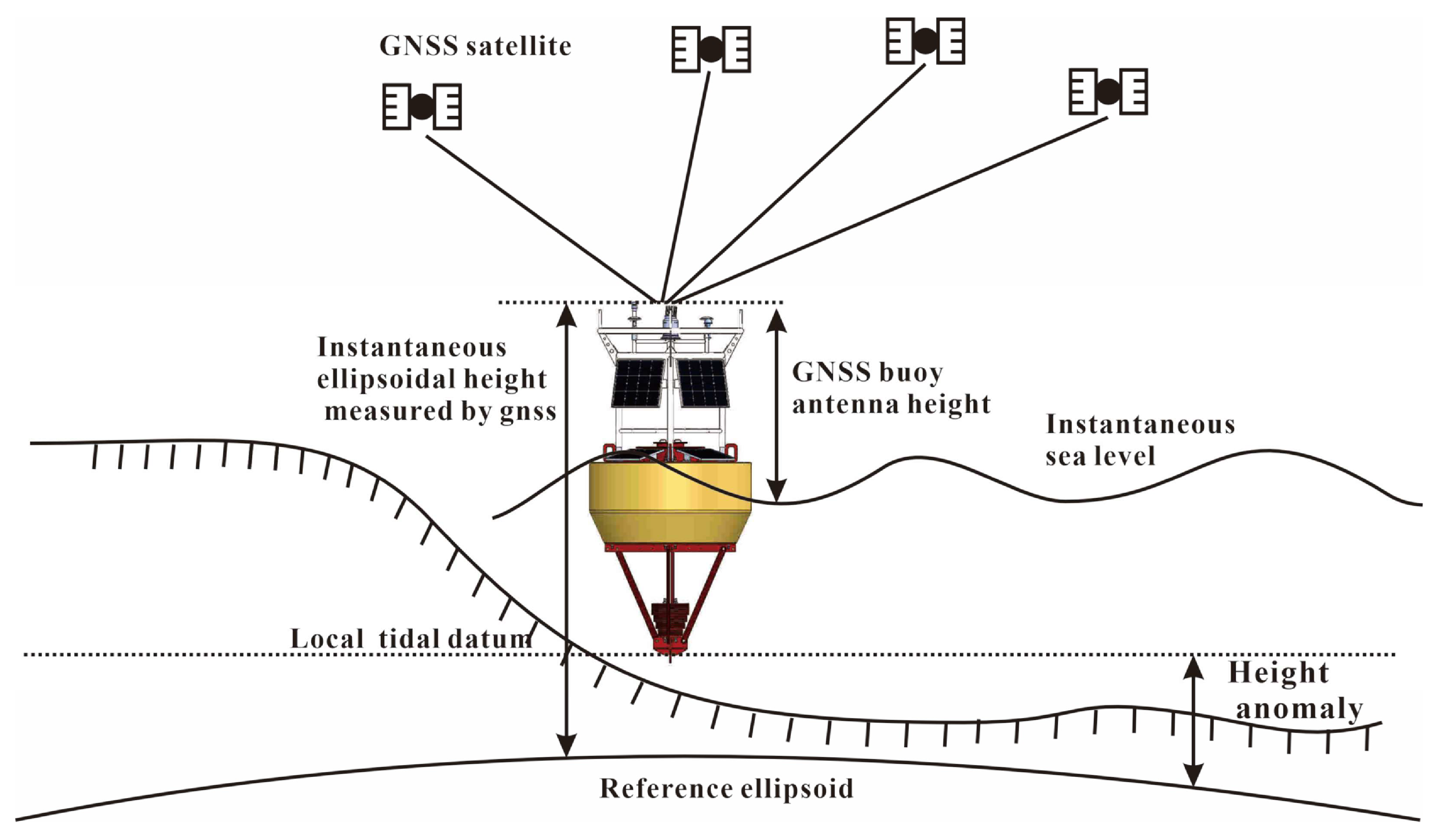
2.1. Principles of GNSS Buoy Tide-Level Measurement

In this study, we developed a GNSS buoy with precise-point-positioning (PPP) measurement technique. This technique utilizes GNSS carrier phase and pseudorange observations, employing high-precision satellite orbit and clock correction products [13,14]. Through model adjustments or parameter estimation methods, it meticulously handles errors related to the satellite end, signal propagation path, and instrument end, which achieves high-precision positioning [15,16,17]. The principle of its tide measurement is as shown in Figure 1. Compared to other commonly used offshore tide measurement methods such as bottom-mounted pressure and acoustic sensors, the tide measurements from this GNSS buoy are based on the CGCS2000 (China Geodetic Coordinate System 2000) co-ordinate system [18]. The CGCS2000 is a geodetic co-ordinate system developed by China. It is a national standard for geodetic surveys and mapping in China. The system is based on the Earth’s geometric ellipsoid and uses the International Terrestrial Reference Frame (ITRF) as its foundation.

These measurements can be converted to tide levels under other absolute elevation reference systems, such as China’s 1985 National Elevation Datum. This type of sea surface elevation data can be directly employed in tasks including the design and construction of offshore wind farms.

The harsh marine environment can lead to excessive swaying of the buoy, causing the GNSS signal to lose lock and, consequently, reducing the accuracy of tide measurements. The operation of high-precision single-point positioning requires the buoy to store a substantial amount of raw GNSS observation data. In this study, a cylindrical buoy with a diameter of 2.3 m was designed, optimized, and manufactured based on the results of stability calculations of the buoy’s numerical model and hydrodynamic computations. Based on the GNSS sensor, attitude sensor, and satellite communication equipment mounted on the buoy, a high-capacity and stable buoy data acquisition unit was developed as an embedded data collection platform. The developed buoy involves comprehensive analysis of the GNSS measurement principles, the operational state of the buoy in the ocean, and the data from various sensors. Accordingly, a sea surface elevation data processing workflow was developed for the GNSS buoy to determine tide levels under an absolute elevation reference system. As a result, the application of the GNSS buoy for long-term tide measurements in an offshore wind farm located over 70 nautical miles from the coast has been successfully achieved.

2.2. Procedure of Data Processing

While the GNSS buoy operates at sea in a long-term manner, severe weather conditions (e.g., strong winds and heavy rainfall) can degrade the precision of GNSS OEM board’s satellite signal reception. As a result, the accuracy of sea surface elevation measurements could be diminished significantly. This study employs the following steps to process the buoy’s GNSS observation data, ensuring the accuracy of unceasingly long-term sea surface elevation measurements:

• Using the PPP technique to calculate the GNSS antenna phase center height involves the following steps: (a) combining the precise ephemeris and clock data provided by the International GNSS Service (IGS) with the GNSS observation data collected from the buoy’s antenna in Receiver Independent Exchange Format (RENIX) format; and (b) Employing Inertial Explorer software (Version 8.90) developed by NovAtel (Calgary, Canada) for data processing. Through this process, the precise three-dimensional co-ordinates of the observation station are obtained.
• During this data processing, some observed data may exhibit poor quality, causing difficulties in fixing the integer ambiguities in the carrier phase observations. This can result in gross errors in the final outputs, particularly in the elevation component. To address the issue, LARISA criteria are employed to diminish the errors of elevation data. Specifically, we first calculate the average elevation value $\overline{\mathrm{X}}$ and the standard deviation (σ) of the elevation data for each 1 min interval. If the value, ${\mathrm{X}}_{\mathrm{i}}$, satisfies the condition $\left|{\mathrm{X}}_{\mathrm{i}}-\overline{\mathrm{X}}\right|>3\mathsf{\sigma }$, then it is considered a gross error and will be discarded.
• To better mitigate the multipath effects on GNSS receiver antennae, GNSS antennae are typically installed at a certain distance above the sea surface. Therefore, the GNSS receiver antenna’s phase height needs to be calibrated using attitude data to obtain the instantaneous sea surface elevation in the area. This measurement is achieved by the sea surface elevation measurement equipment. The formula is shown as follows:

$${ E}_{ss}={ E}_{APC}-D\cos \epsilon \cos \theta$$

(1)

Specifically, $E_{ss}$ indicates the instantaneous sea surface elevation measured by the equipment. The GNSS antenna phase center height is represented by $E_{APC}$. $D$ is the distance between the GNSS antenna and the sea surface when the equipment is in a stationary state. $\epsilon$ and $\theta$ denote the instantaneous roll and pitch of the equipment.

4.

The obtained instantaneous sea surface elevation is then subjected to a Kalman filter to remove high-frequency signals (i.e., wave motion and noise) [19]. The Kalman algorithm is a filtering technique based on a state-space model. It models the signal as a state variable and continuously adjusts the estimated value of the state variable to improve the accuracy of observations. The Kalman filter parameters are defined as follows: state transition matrix: $[1dt;0 1]$; observation matrix: $[1 0]$; state transition noise covariance matrix: $[0.01 0;0 0.001]$; and observation noise variance: $0.1$.

5.

The sea surface elevation obtained from the GNSS buoy measurements corresponds to geodetic height. It takes ellipsoidal surface as the elevation reference. Currently, sea surface elevation observations are typically referenced against the China National Height Datum 1985 (CNHD 1985). Sea surface elevation can be calculated by subtracting the observed geodetic height from the elevation anomaly of the observed sea area. The elevation anomaly of the observed sea area can be determined by using the EGM2008 model [20]. The EGM2008 is a spherical harmonic model of the Earth’s gravitational potential, developed by the National Geospatial-Intelligence Agency of the United States (Springfield, the United States). It has been developed over years by building upon previous experiences and theoretical foundations in constructing Earth’s gravity field models. The model utilizes the PGM2007B as a reference model and integrates gravity data collected from the GRACE (Gravity Recovery and Climate Experiment) satellites, along with global 5′ × 5′ gravity anomaly data.

2.3. Buoy Body Design

As shown in Figure 2, the buoy body consists of the upper structure, buoyancy body and instrument compartment, and lower structure. The upper structure carries the GNSS antenna, satellite communication terminal, Airmar automatic weather station, and anchor light. The upper body is made of cast aluminum. This ensures both the strength of the upper structure and the advantage of low density, which helps lower the overall center of gravity and improve buoy stability. The buoyancy body is made from PE material with a surface coating of polyurethane to provide sufficient strength and corrosion resistance.

The instrument compartment houses the data acquisition unit, solar charging controller, and data acquisition components, all made from 316L stainless steel. The lower structure supports the entire buoy and includes ballast, sacrificial anodes, and anchoring equipment. The anchoring system consists of anchor chain, anchor rope, acoustic release, gravity anchor, and swivel. It can be adjusted by varying the length of the anchor rope to accommodate different water depths.

The three-dimensional model of the buoy was created through SolidWorks software (Version 2018) where the decisive design parameters are obtained from the statistics functions of the software. The main parameters for the buoy are indicated in

Table 1. Main parameters of buoy.

Parameter	Value
Design diameter	2.30 m
Design mass	$2.45\times {10}^3$ kg
Design height	5.11 m
Reserved buoyancy	$3.12\times {10}^3$ kg
Center of gravity height	1.23 m
Buoyant center height	1.26 m
Draft height	1.55 m
Buoy projected area normal to the wind	3.29 m2
Buoy projected area normal to the flow	2.53 m2
x-axis moment of inertia (CG)	$2.39\times {10}^3$ kg∙m2
y-axis moment of inertia (CG)	$2.39\times {10}^3$ kg∙m2
z-axis moment of inertia (CG)	$1.94\times {10}^3$ kg∙m2

.

According to marine industry standard “Small mooring buoy system for ocean observing” (HY/T143—2011) [21], the buoy limit living environment parameters are shown in

Table 2. Buoy limit living environment parameters.

Parameter	Value
Wind speed	60.0 m/s
Wave period	12.0 s
Wavelength	224 m
Significant wave height	15.0 m
Maximum wave height	20.0 m
Surface current speed	3.50 m/s

. These parameters are designated to adapt to China’s offshore sea conditions.

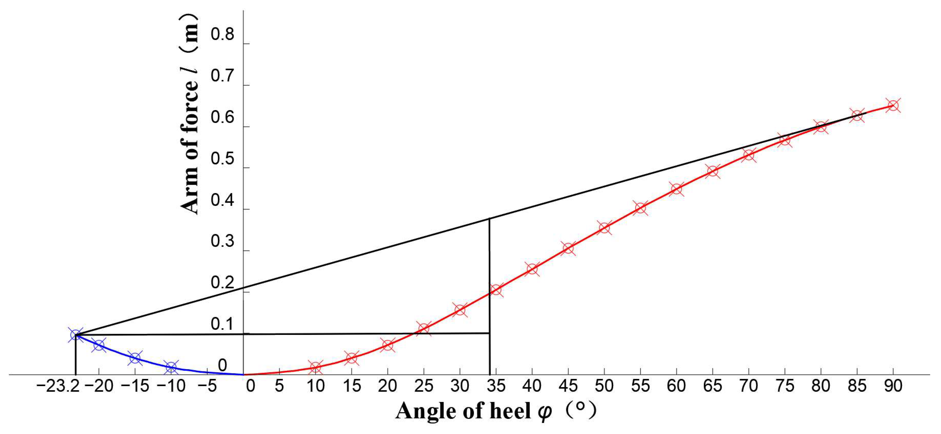
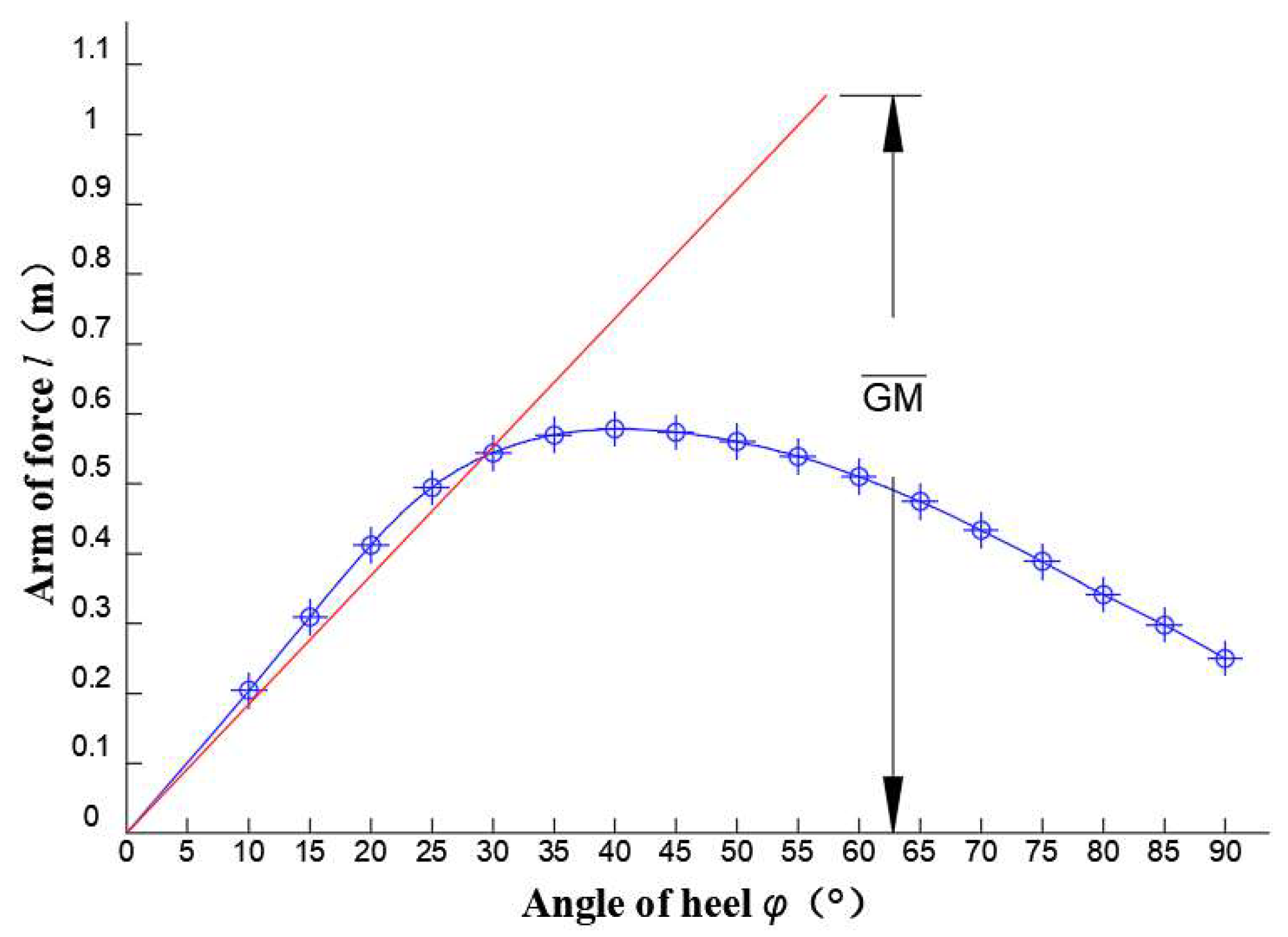
2.4. Buoy Stability Calculation

Buoy stability calculation is conducted to assess the buoy’s ability to return to its equilibrium position after being subjected to external forces [22,23]. This evaluation encompasses both initial stability and high-angle stability: (1) Initial stability generally refers to the stability when the inclination angle is less than 10–15° or before the deck edge starts submerging. (2) High-angle stability pertains to stability when the inclination angle is greater than 10–15° or after the deck edge starts submerging [24,25]. The results of initial stability calculation include the buoy’s initial metacentric height, inherent roll period, and maximum roll angle. For high-angle stability, the process begins with calculating the buoy’s static stability arm curve using the variable displacement method. This curve is then integrated to obtain the dynamic stability arm curve of the buoy. Based on the static stability arm curve, we can determine the parameters, such as the maximum static heel angle, maximum restoring arm, and stability lost angle. Similarly, the dynamic stability arm curve provides parameters like the maximum dynamic roll angle, minimum capsizing arm, and stability criterion number.

At last, the buoy’s design has been further optimized by thoroughly comparing the results of the buoy stability calculations and the requirements outlined in the “Technical Rules for Statutory Inspection of Domestic Navigational Ships” [26]. The buoy stability calculation results are as follows (Figure 3 and Figure 4):

• Initial metacentric height: 1.056 m;
• Metacentric radius: 1.033 m;
• Natural roll period (free): 5.2 s;
• Maximum free roll angle: 15.3°;
• Maximum restoring arm: 0.58 m;
• Ultimate roll angle: 41°;
• Stability lost angle: >90°;
• Minimum capsizing arm: 0.27 m;
• Stability criterion number: 1.26.

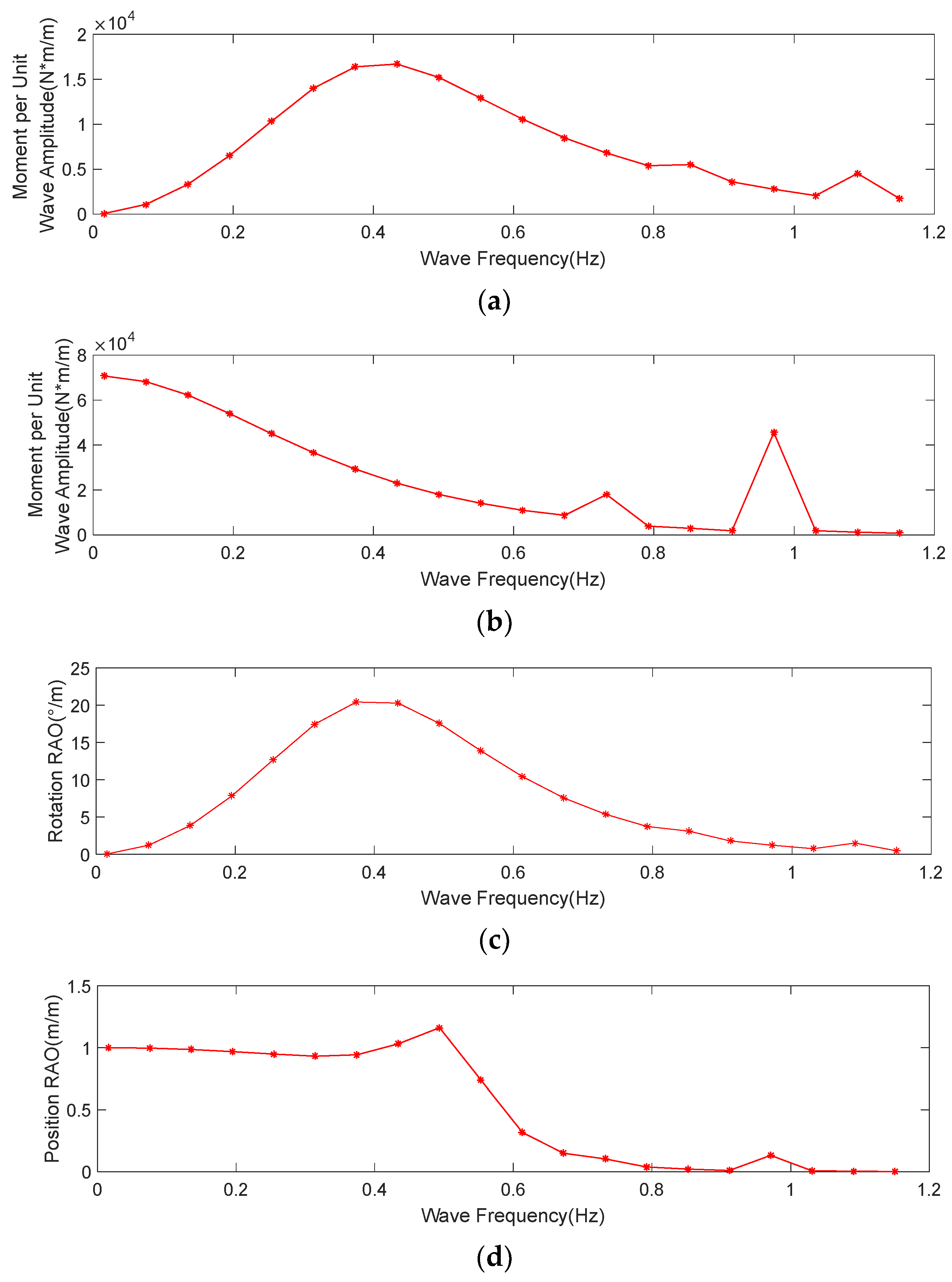
2.5. Buoy Hydrodynamic Analysis

The hydrodynamic analysis for the buoy is based on three-dimensional potential flow theory and wave radiation–diffraction theory. This analysis examines the buoy’s motion response to wind, wave, and current loads in the ocean environment [27]. The buoy exhibits translational and rotational motion along three co-ordinate axes in seawater, resulting in a total of six degrees of freedom of movement. These are termed as sway, heave, surge, roll, pitch, and yaw. The co-ordinate origin is set at the buoy’s center of gravity. Due to the nearly symmetrical design of the buoy, the yawing motion of the buoy is minimally affected by waves. Therefore, the focus is solely on the buoy’s horizontal sway, roll motion, and vertical heave motion in the research. The buoy’s hydrodynamic analysis in the frequency domain is conducted using the Advanced Quantitative Wave Analysis (AQWA) software (Version 19.0). Especially, the calculations employed Joint North Sea Wave Project (JONSWAP) spectrum which is an embedded function of the AQWA software. The wave frequency range is lastly specified as 0 to 1.2 Hz [28,29].

Potential flow theory, in fact, neglects the impact of fluid viscosity on the buoy’s motion during simulations. Therefore, before conducting the simulation calculations, it is necessary to adjust the damping associated with the three-dimensional potential flow theory to account for this oversight. The simulation calculations have provided the first-order wave forces acting on the buoy during horizontal and vertical translational motion. The simulation also involves the variation curves of the response amplitude operators (RAOs) for horizontal rotation and vertical translation motion in relation to wave frequency. Specifically, first-order wave forces represent the effect of wave loads on the ocean buoy, indicating the forces exerted by wave-induced loads on the buoy. RAOs are defined as the transfer functions that describe the response of a floating body’s motion to wave excitation. They represent the ratio of the amplitude of the floating body’s motion to the amplitude of the incident wave. In other words, RAOs indicate the characteristics of the floating body’s motion response under linear wave conditions.

As shown in Figure 4, the wave forces applied on the buoy in the horizontal direction exhibit a growth at first, followed by a falling. The maximum value of wave force per unit under significant wave height is 16,683.46 N at the frequency of 0.4338 Hz. This pattern indicates that the buoy experiences lower forces in good sea conditions. As the sea conditions deteriorate, the wave forces gradually increase. However, the amplitude of wave forces is increased in a gradual fashion. Meanwhile, we do not observe the sharp spikes at any specific frequencies. The vertical wave forces experienced by the buoy also decrease gradually and smoothly as the wave frequency increases. However, the magnitude of these wave forces is significantly high, indicating that the buoy exhibits substantial motion response in the heave direction.

Moreover, the buoy’s response in terms of sway and heave becomes minimal after the wave frequency exceeds 0.75 Hz (see Figure 5). When the wave frequency is below 0.75 Hz, the buoy’s responses in sway and heave gradually strengthen with the increase of the wave frequency. The sway RAO reaches its maximum value of 20.45°/m around 0.37 Hz. The RAO values in heave change smoothly when the wave frequency is below 0.75 Hz. In contrast, all RAO values significantly increase beyond 0.75 Hz, peaking at 1.16 m/m around 0.49 Hz. In brief, the RAO results express that the responses in sway and heave directions are relatively small, and their changes with frequency are relatively smooth without any sharp spikes.

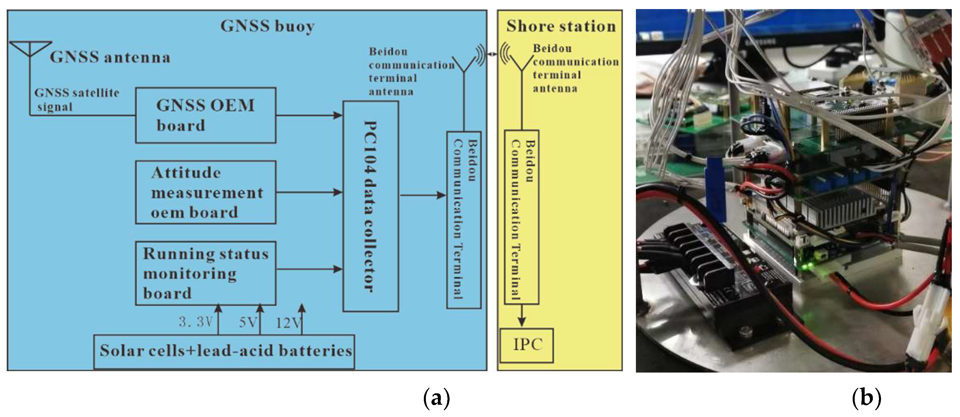
2.6. Development of Buoy Data Acquisition Unit

The buoy data acquisition unit consists of both the buoy data acquisition device and the shore station. The buoy data acquisition device is installed within a sealed compartment on the buoy. It is designed to collect and store various types of data, including raw GNSS observation data, dynamic draft data, and buoy’s dynamic attitude data. The collected data are then encoded and transmitted via the BeiDou communication terminal to the shore station. The primary function of this unit is to acquire the operational status of the data acquisition device, as well as to encode and transmit specific sensor data to the shore station for further analysis and processing. The buoy data acquisition unit is composed of several components, including a GNSS OEM board, attitude measurement board, pressure-based depth gauge, voltage conversion board, embedded data acquisition device, and BeiDou communication terminal (shown in Figure 6). The GNSS OEM board used in the system is the OEM729 model from NovAtel. This board provides GNSS raw observation data at an update rate of 5 Hz. Through post-processing and calculation, the buoy’s latitude, longitude, and elevation are derived. The employed attitude measurement board is the TCM2.5 model from PNI. This board measures the buoy’s dynamic roll, pitch, and yaw angles. Regarding the pressure-based depth gauge, we selected the DW1122 model from DAOWAN. It measures the buoy’s dynamic draft depth. The embedded data acquisition device equipped in the system is the PCM3365 model from YANHUA. It is a small-size stackable embedded acquisition device based on the PC104 bus architecture. It features a 1 TB solid-state drive for storage, effectively meeting the high speed, extensive data collection, storage, and processing needs of the GNSS buoy. The shore station for the buoy consists of a BeiDou communication terminal and an industrial computer. It is responsible for receiving the information transmitted by the buoy’s data acquisition device. The shore station then performs the tasks of parsing, displaying, and storing the received data.

3. Results

This chapter first introduces the prototype of the developed buoy and the experimental overview. Second, the GNSS buoy data-processing workflow is further described. Finally, the experimental results are discussed by the end of the chapter.

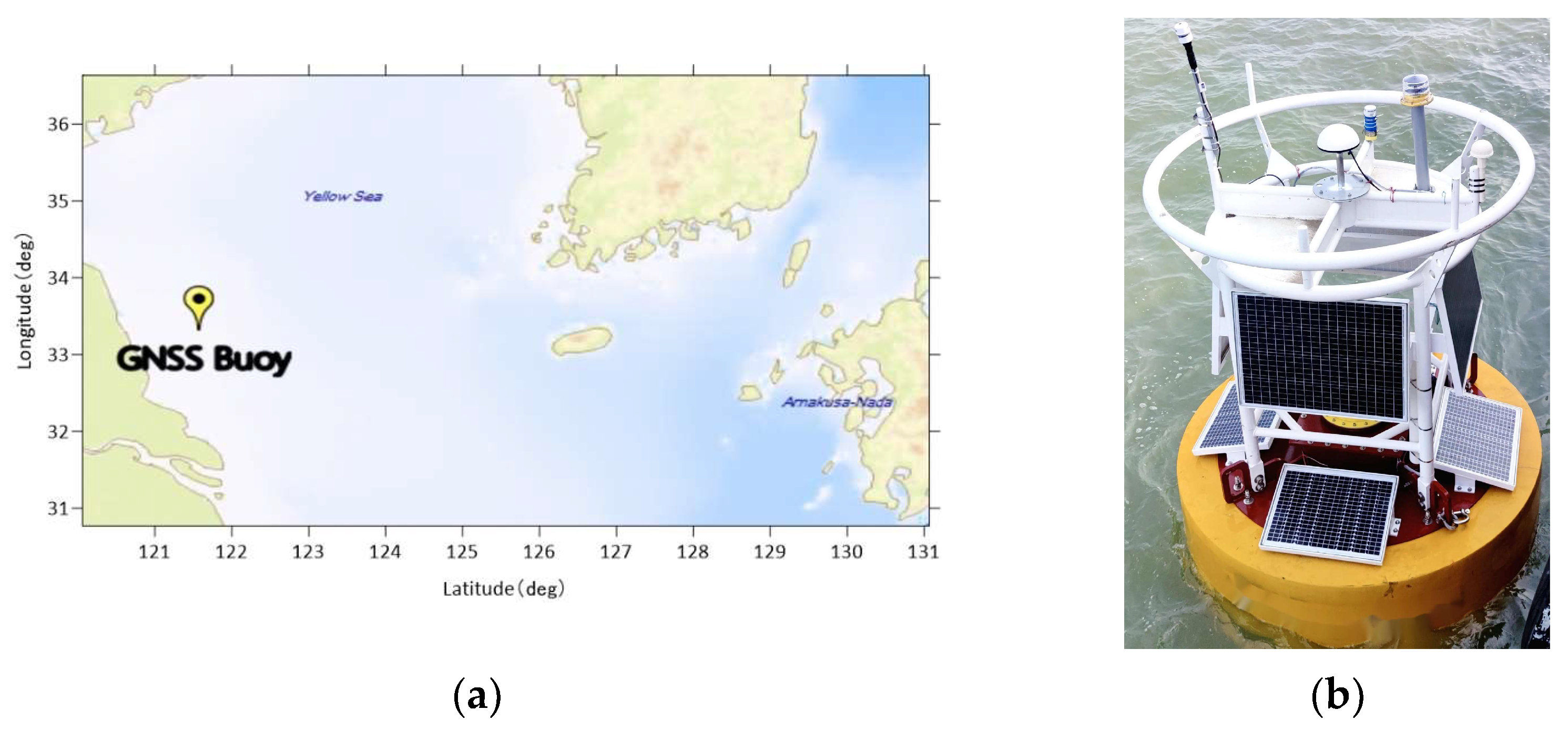
3.1. Performance Evaluation on Sea Trial

On 6 August 2022, the developed buoy was deployed in the offshore wind farm area (33.3416°N, 121.5933°W) approximately 70 km off the coast of Jiangsu, the Yellow Sea, in China (as shown in Figure 7), and the pressure sensor was deployed on the seabed near the buoy’s anchor.

The sea level oscillations in the Yellow Sea exhibit diverse fluctuations predominantly due to tidal and atmospheric influences. Tidal movements are primarily governed by lunar and solar gravitational forces. Typically, the average tidal range in this region spans between 2 to 4 m, subject to local geography and bathymetry alterations. Notably, extreme tidal ranges occur during spring tides when the gravitational forces align, leading to higher high tides and lower low tides, surpassing the average range by several meters.

Moreover, atmospheric dynamics, including storm surges and wind-induced shifts, significantly impact sea-level changes in the Yellow Sea. Storm surges, prompted by intense low-pressure systems or strong winds, cause abrupt and substantial sea-level elevations, potentially resulting in coastal flooding.

The interplay of these tidal and atmospheric influences shapes the sea-level oscillations in the Yellow Sea, crafting a dynamic marine environment with fluctuations in both mean and extreme sea levels [30].

Specifically, the equipment operated independently for two months for the sea surface elevation measurements. Through immersion testing of the buoy’s body and pressure testing of the buoy’s instrument compartment, the buoy’s self-stability and sealing performance were confirmed to meet requirements. The technical specifications are detailed in

Table 3. Main technical specifications of model.

Parameter	Value
Buoy mass	$2.49\times {10}^3$ kg
Antenna height	2.21 m
Operating temperature	−20.0~80.0 °C
GNSS signals	GPS: L1, L2, L5, GPS: L1 C/A, L1C, L2C, L2P, L5 BeiDou: B1, B2, B3 GLONASS: L1 C/A, L2C, L2P, L3, L5
Attitude accuracy	Roll/Pitch: 0.200°
GNSS data update rate	5.00 Hz
Attitude data update rate	5.00 Hz

. In addition, a bottom-mounted pressure tide gauge was also deployed in the trial area for synchronous observations.

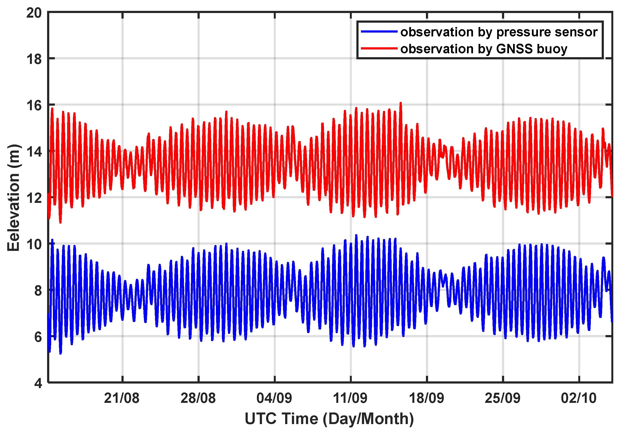
3.2. Marine Test Results

As shown in Figure 8, the GNSS buoy moves in a circular path around the mooring system, with a maximum movement radius of 31.924 m. To meet the observation requirements of offshore wind farms for sea level, the sea level data acquired by both the GNSS buoy and the pressure sensor are processed at one-hour intervals, as depicted in Figure 9, The sea level elevation measured by the GNSS buoy is based on the CGCS2000 co-ordinate system and can be converted to the 1985 national elevation datum. This measurement is the absolute elevation. The sea level measured by the pressure sensor is relative to the sensor’s own reference zero point, representing the relative elevation. As their elevation reference points differ, the two curves do not overlap, yet they exhibit similar changing trends.

The comparison of the GNSS buoy and the pressure sensor for measuring the sea level elevation is shown in Figure 10; the red solid line is the relationship equation between the GNSS buoy and the pressure sensor measurements obtained through polynomial fitting, which is $Y=0.9556X+5.9266$. The slope of the equation is 0.9556. If the slope of the equation is 1, it indicates that the measurements of the GNSS buoy and the pressure sensor are identical. The observation of the relationship equation between the GNSS buoy and the pressure sensor shows a slope value that differs very little from 1. Furthermore, the calculated correlation coefficient between the two is 0.99. The above results indicate a strong correlation between the measurements of the GNSS buoy and the pressure sensor.

By performing the harmonic analysis separately for both datasets, the harmonic constants for the eight major constituents are determined [31], as shown in

Table 4. The amplitudes and phases of the 8 tidal components of GNSS buoys and pressure sensors.

		O1	P1	K1	Q1	M2	N2	S2	K2
Amplitude (cm)	GNSS buoy	16.1	6.1	20.4	2.8	137.7	20.8	58.8	21.2
	Pressure sensor	16.7	6.7	21.6	3.9	138.9	20.7	57.5	22.1
	Difference	−0.6	−0.6	−1.2	−1.2	−1.2	0.1	1.4	−1.0
Phase (°)	GNSS buoy	257.0	293.6	326.4	168.1	96.9	63.2	130.1	155.7
	Pressure sensor	258.3	300.0	329.3	180.3	95.1	63.5	127.9	143.4
	Difference	−1.3	−6.4	−2.9	−12.2	1.8	−0.3	2.2	12.3

and Figure 11; the semi-diurnal tide is in the dominant status. In the presence of the eight tidal constituents (O₁, P₁, K₁, Q₁, M₂, N₂, S₂, and K₂), K₁, O₁, M₂, and S₂ are the main tidal constituents, and the influence of the M₂ tidal constituent is the most significant. The amplitudes of the tidal constituents O₁, P₁, K₁, Q₁, M₂, N₂, S₂, and K₂ obtained through the harmonic analysis of the buoy data are as follows: O₁: 16.1 cm, P₁: 6.1 cm, K₁: 20.4 cm, Q₁: 2.8 cm, M₂: 137.7 cm, N₂: 20.8 cm, S₂: 58.8 cm, and K₂: 21.2 cm. The phases of the tidal constituents are as follows: O₁: 257.0°, P₁: 293.6°, K₁: 326.4°, Q₁: 168.1°, M₂: 96.9°, N₂: 63.2°, S₂: 130.1°, and K₂: 155.7°. On the other hand, the amplitudes and phases of the tidal constituents obtained from the harmonic analysis of the pressure sensor data are as follows: amplitudes: O₁: 16.7 cm, P₁: 6.7 cm, K₁: 21.6 cm, Q₁: 3.9 cm, M₂: 138.9 cm, N₂: 20.7 cm, S₂: 57.5 cm, and K₂: 22.1 cm; and phases: O₁: 258.3°, P₁: 293.6°, K₁: 300.0°, Q₁: 180.3°, M₂: 95.1°, N₂: 63.5°, S₂: 127.9°, and K₂: 143.4°.

Comparing the results of the harmonic analysis between the two datasets, the differences in amplitudes and phase angles for the four main tidal constituents can be found easily. The amplitude difference for the M₂ tidal constituent is −1.2 cm, and the phase difference is 1.8°. Regarding O₁, the amplitude difference is −0.6 cm, and the phase difference is −1.3°. The amplitude and phase difference for the K₁ tidal constituent is −1.2 cm and −2.9°, respectively. The amplitude difference for the S₂ tidal constituent is 1.4 cm, and the phase difference is 2.2°. From the results, it can be concluded that the harmonic analysis results from both sources are generally consistent. This indicates a high degree of agreement between the tidal data obtained from the GNSS buoy observations and the pressure sensor observations.

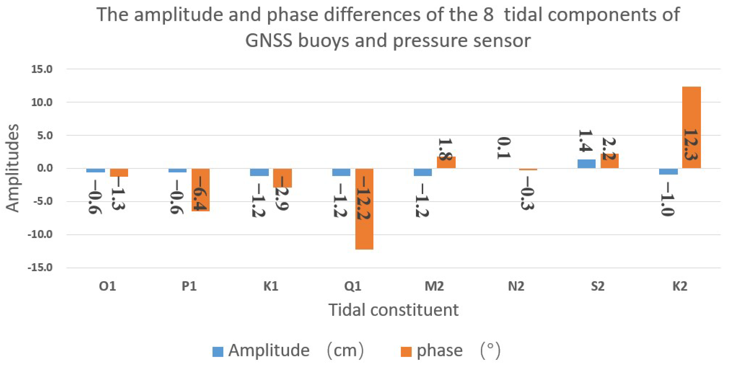
3.3. Uncertainty Evaluation of Sea Surface Elevation

In order to assess the reliability of the measurements obtained from the GNSS tide buoy and clarify the sources of uncertainty in the measurement process of the GNSS tide buoy, ensuring its capability to provide accurate and reliable tidal information for various marine engineering requirements, this study conducted an uncertainty assessment of the measurements from the GNSS tide buoy [32]. From a metrological perspective, the measurement system, the measurement environment, and the measured object in the GNSS buoy measurement process exhibit temporal, stochastic, and correlated characteristics, making it a dynamic measurement process.

Based on the operating principles, system components, data-processing methods, and marine experiments of the GNSS tide buoy, this study decomposed the dynamic measurement process of the GNSS tide buoy into a set of static measurement processes. Using the GUM (Guide to the Expression of Uncertainty in Measurement) approach, a measurement model was established, and the uncertainty components of the instantaneous sea surface elevation in the static measurement process were analyzed and calculated in detail, including the GNSS instantaneous elevation uncertainty, the GNSS antenna height correction uncertainty, and the elevation anomaly uncertainty. Finally, the dynamic standard uncertainty and dynamic expanded uncertainty of the instantaneous sea surface elevation were synthesized. Some computational results are presented in Figure 12 below. The red line in the figure represents the dynamic combined standard uncertainty of the tide level measured by the GNSS buoy. The curve amplitude is reasonable and there are few abnormal points, indicating that the tide level results measured by the GNSS buoy have a considerable degree of reliability.

During the uncertainty assessment process, three dynamic uncertainty components were analyzed and calculated. It is evident from this that the primary sources of uncertainty in the measurement results of the GNSS tide buoy are related to the measurement capabilities of the sensors, the stability of the floating body, the marine environment where the buoy is located, and the accuracy of the elevation anomaly calculation model. Subsequent work can focus on optimizing the GNSS tide buoy from these aspects.

4. Discussion

The ultimate goal of this study is to develop the GNSS buoy technology into a mature ocean tidal measurement technique capable of facilitating various marine engineering operations. The current development and oceanic tests have preliminarily verified the feasibility of this technology. However, numerous issues have been identified that urgently require resolution during the testing process.

4.1. The Influence of GNSS Buoy Data Collection Approach on Measurement Results

The developed GNSS buoy measures instantaneous sea surface elevations by collecting GNSS raw observation data and buoy attitude data to calculate the tidal observation results. The minimum period of ocean tides is approximately 12 h. Following the Nyquist sampling theorem, considering the storage space of the buoy’s data collector and its impact on the buoy’s operational duration, the GNSS raw observation data’s sampling rate is set at 5 Hz. A higher data-sampling rate can prevent signal aliasing, obtain more precise spectral information, and ensure the accurate sampling and reconstruction of instantaneous sea surface elevation data. However, it also introduces the issue of increased data volume. The GNSS OEM board used in this study has a maximum data sampling rate of 10 Hz. Subsequent experiments will utilize 10 Hz GNSS data for tidal measurements to compare the degree of increased data accuracy due to higher sampling rates and the increased storage costs of the buoy data collector, to determine whether to use a higher data acquisition rate.

The GNSS buoy operates as a dynamic platform measurement, and the platform’s movements affect the measurement outcomes. Based on experimental observations, the oscillations caused by ocean waves influence the computation process from the GNSS antenna’s phase center height to the instantaneous sea surface elevation. Moreover, the lateral displacement caused by ocean currents prevents the buoy from measuring at a fixed point, decreasing the accuracy of maximum tidal range measurements. Consequently, this study plans to incorporate wave and current measurement sensors onto the buoy to investigate the impact of waves and currents on the precision of tidal measurements by the GNSS buoy. Additionally, it aims to develop corresponding algorithms to enhance data accuracy.

4.2. The Impact of Float Design and Simulation on Technological Applications

The cyclical occurrence of severe oceanic weather conditions and unpredictable human-induced disruptions are significant factors affecting the long-term operation of the GNSS tide measurement buoy. Harsh sea conditions can lead to anchor failure and the drifting of the buoy. A time-domain mooring analysis will be conducted to optimize the buoy’s mooring system. In the targeted area of this study, human-induced disruptions are relatively common. The experiment lasted only 60 days due to deliberate damage to the buoy’s solar power system, as shown in the Figure 13. Consequently, the robust design of the buoy’s sensor installation structure and the implementation of protective barriers and warning systems during buoy deployment are crucial aspects for future work.

4.3. Real-Time Sea Surface Elevation Measurements by GNSS Buoy

The requirements for annual tidal observations in offshore wind farms demand real-time data. Therefore, this study employs a GNSS post-processing algorithm to compute buoy data. One of the prevailing trends in marine observation is real-time monitoring. The real-time observations of the GNSS tide measurement buoy rely on GNSS real-time data-processing algorithms. Presently, some mature GNSS real-time data-processing algorithms include real-time kinematic (RTK) and base station differential solutions. RTK typically operates effectively within a distance of approximately 10 km, rendering it unsuitable for the working area of the GNSS buoy in this study. The GNSS OEM board utilized in this study supports TerraSTAR-C technology. TerraSTAR-C is a precise positioning service provided by TerraStar, a global navigation satellite systems (GNSS) corrections and positioning services provider. Subsequent work will involve research on real-time tide measurement technology based on TerraSTAR-C and determine the precision of this technology for tidal measurements.

5. Conclusions

A GNSS buoy is a relatively new method for tidal measurement. To enable long-term operation in open sea areas (e.g., offshore wind farms) and to convert the measured tidal data into local elevation references, this study addressed the following tasks: (1) performing stability and hydrodynamic calculations on the buoy to enhance its posture response in complex sea conditions, as well as reducing the occurrence frequency of GNSS satellite signal loss during extended periods of marine operations; (2) developing a high-performance, large-capacity data logger for the buoy to ensure that it can continuously collect all necessary data over an extended period; and (3) determining the GNSS buoy data-processing workflow based on practical working conditions to ensure the accuracy of the GNSS buoy tidal measurements. The tidal measurement results obtained from the developed GNSS buoy show high consistency to the measurements from the bottom-mounted pressure sensors near the buoy. The harmonic analysis of the results indicates that the differences in amplitude and phase angle for the major tidal constituents (i.e., M₂ and S₂) between the two measurement methods are minimal. In summary, the strong correlation between the measurement results of the GNSS buoy and pressure sensor, and the relatively small differences in the amplitude and phase of the main tidal components indicate that the compact GNSS buoy has the ability to continuously measure the sea surface elevation with an elevation reference and the tide level in the open sea, providing technical support for offshore engineering.

References

1. Ko, D.H.; Jeong, S.T.; Cho, H.-Y.; Kang, K.-S. Analysis on the estimation errors of the lowest and highest astronomical tides for the southwestern 2.5 GW offshore wind farm, Korea. Int. J. Nav. Archit. Ocean Eng. 2018, 10, 85–94. [Google Scholar] [CrossRef]
2. Christie, E.; Li, M.; Moulinec, C. Comparison of 2D and 3D large scale morphological modeling of offshore wind farms using HPC. Coast. Eng. Proc. 2012, 1, 42–48. [Google Scholar] [CrossRef]
3. Loughney, S.; Wang, J.; Bashir, M.; Armin, M.; Yang, Y. Development and application of a multiple-attribute decision-analysis methodology for site selection of floating offshore wind farms on the UK Continental Shelf. Sustain. Energy Technol. Assess. 2021, 47, 101440. [Google Scholar] [CrossRef]
4. Yu, Y.; Mi, Z.Q.; Liu, X.J.; Sun, L. Modeling method of large-scale wind farm based on operating data. Acta Energiae Solaris Sin. 2011, 32, 1543–1548. [Google Scholar]
5. Díaz, H.; Soares, C.G. An integrated GIS approach for site selection of floating offshore wind farms in the Atlantic continental European coastline. Renew. Sustain. Energy Rev. 2020, 134, 110328. [Google Scholar] [CrossRef]
6. Giardina, M.F.; Earle, M.D.; Cranford, J.C.; Osiecki, D.A. Development of a Low-Cost Tide Gauge. J. Atmos. Ocean. Technol. 2000, 17, 575–583. [Google Scholar] [CrossRef]
7. Míguez, B.M.; Testut, L.; Wöppelmann, G. Performance of modern tide gauges: Towards mm-level accuracy. Sci. Mar. 2012, 76, 221–228. [Google Scholar] [CrossRef]
8. Dawidowicz, K. Sea level changes monitoring using GNSS technology—A review of recent efforts. Acta Adriat. 2014, 55, 145–161. [Google Scholar]
9. Knight, P.J.; Bird, C.O.; Sinclair, A.; Higham, J.; Plater, A.J. Beach Deployment of a Low-Cost GNSS Buoy for Determining Sea-Level and Wave Characteristics. Geosciences 2021, 11, 494. [Google Scholar] [CrossRef]
10. Chupin, C.; Ballu, V.; Testut, L.; Tranchant, Y.-T.; Calzas, M.; Poirier, E.; Coulombier, T.; Laurain, O.; Bonnefond, P.; Team FOAM Project. Mapping Sea Surface Height Using New Concepts of Kinematic GNSS Instruments. Remote Sens. 2020, 12, 2656. [Google Scholar] [CrossRef]
11. Lin, Y.-P.; Huang, C.-J.; Chen, S.-H.; Doong, D.-J.; Kao, C.C. Development of a GNSS Buoy for Monitoring Water Surface Elevations in Estuaries and Coastal Areas. Sensors 2017, 17, 172. [Google Scholar] [CrossRef] [PubMed]
12. Kato, T.; Terada, Y.; Tadokoro, K.; Futamura, A. Developments of GNSS buoy for a synthetic geohazard monitoring system. Proc. Jpn. Acad. Ser. B 2022, 98, 49–71. [Google Scholar] [CrossRef] [PubMed]
13. Herbers, T.H.C.; Jessen, P.F.; Janssen, T.T.; Colbert, D.B.; MacMahan, J.H. Observing Ocean Surface Waves with GPS-Tracked Buoys. J. Atmos. Ocean. Technol. 2012, 29, 944–959. [Google Scholar] [CrossRef]
14. Chung-Yen, K.; Kuan-Wei, C.; Kai-Wei, C.; Kai-Chien, C.; Li-Ching, L.; Hong-Zeng, T.; Hsiang-Tseng, L. High-frequency sea level variations observed by GPS buoys using precise point positioning technique. TAO Terr. Atmos. Ocean. Sci. 2012, 23, 209. [Google Scholar]
15. Ma, H.; Zhao, Q.; Verhagen, S.; Psychas, D.; Liu, X. Assessing the Performance of Multi-GNSS PPP-RTK in the Local Area. Remote Sens. 2020, 12, 3343. [Google Scholar] [CrossRef]
16. Yigit, C.O.; Gurlek, E. Experimental testing of high-rate GNSS precise point positioning (PPP) method for detecting dynamic vertical displacement response of engineering structures. Geomat. Nat. Hazards Risk 2017, 8, 893–904. [Google Scholar] [CrossRef]
17. Hohensinn, R.; Stauffer, R.; Glaner, M.F.; Pinzón, I.D.H.; Vuadens, E.; Rossi, Y.; Clinton, J.; Rothacher, M. Low-Cost GNSS and Real-Time PPP: Assessing the Precision of the u-blox ZED-F9P for Kinematic Monitoring Applications. Remote Sens. 2022, 14, 5100. [Google Scholar] [CrossRef]
18. Jiang, Z.H.; Zhang, P.; Bei, J.Z.; Li, Z.C. Characteristics of the non-linear movement of CORS network in China based on the CGCS2000 frame. Chin. J. Geophys. 2012, 55, 841–850. [Google Scholar]
19. Slobbe, D.C.; Sumihar, J.; Frederikse, T.; Verlaan, M.; Klees, R.; Zijl, F.; Farahani, H.H.; Broekman, R. A Kalman Filter Approach to Realize the Lowest Astronomical Tide Surface. Mar. Geodesy 2017, 41, 44–67. [Google Scholar] [CrossRef]
20. Pavlis, N.K.; Holmes, S.A.; Kenyon, S.C.; Factor, J.K. The development and evaluation of the Earth Gravitational Model 2008 (EGM2008). J. Geophys. Res. Solid Earth 2012, 117, 8916. [Google Scholar] [CrossRef]
21. National Marine Standardization Technical Committee. Small Mooring Buoy System for Ocean Observing: HYT 143-2011; State Oceanic Administration: Beijing, China, 2011; pp. 6–8. [Google Scholar]
22. Wang, Y.-L. Design of a cylindrical buoy for a wave energy converter. Ocean Eng. 2015, 108, 350–355. [Google Scholar] [CrossRef]
23. Shi, H.; Han, Z.; Zhao, C. Numerical study on the optimization design of the conical bottom heaving buoy convertor. Ocean Eng. 2019, 173, 235–243. [Google Scholar] [CrossRef]
24. Zhang, S.; Yang, W.; Xin, Y.; Wang, R.; Li, C.; Cai, D.; Gao, H. Prototype System Design of Mooring Buoy for Seafloor Observation and Construction of Its Communication Link. J. Coast. Res. 2018, 83, 41–49. [Google Scholar] [CrossRef]
25. Arany, L.; Bhattacharya, S. Simplified load estimation and sizing of suction anchors for spar buoy type floating offshore wind turbines. Ocean Eng. 2018, 159, 348–357. [Google Scholar] [CrossRef]
26. Maritime Safety Administration of the People’s Republic of China. Technical Rules for Statutory Inspection of Domestic Navigating Marine Vessels; China Communication Press: Beijing, China, 2011; pp. 212–216. [Google Scholar]
27. Ghafari, H.; Dardel, M. Parametric study of catenary mooring system on the dynamic response of the semi-submersible plaform. Ocean Eng. 2018, 153, 319–332. [Google Scholar] [CrossRef]
28. Bódai, T.; Srinil, N. Performance analysis and optimization of a box-hull wave energy converter concept. Renew. Energy 2015, 81, 551–565. [Google Scholar] [CrossRef]
29. Amaechi, C.V.; Wang, F.; Hou, X.; Ye, J. Strength of submarine hoses in Chinese-lantern configuration from hydrodynamic loads on CALM buoy. Ocean Eng. 2018, 171, 429–442. [Google Scholar] [CrossRef]
30. Liu, K.; Sun, J.; Guo, C.; Yang, Y.; Yu, W.; Wei, Z. Seasonal and Spatial Variations of the M 2 Internal Tide in the Yellow Sea. J. Geophys. Res. Oceans 2019, 124, 1115–1138. [Google Scholar] [CrossRef]
31. Li, S.; Liu, L.; Cai, S.; Wang, G. Tidal harmonic analysis and prediction with least-squares estimation and inaction method. Estuar. Coast. Shelf Sci. 2019, 220, 196–208. [Google Scholar] [CrossRef]
32. Mauder, M.; Cuntz, M.; Drüe, C.; Graf, A.; Rebmann, C.; Schmid, H.P.; Schmidt, M.; Steinbrecher, R. A strategy for quality and uncertainty assessment of long-term eddy-covariance measurements. Agric. For. Meteorol. 2013, 169, 122–135. [Google Scholar] [CrossRef]
Figure 1. The principle of measuring sea level elevation with elevation reference using GNSS buoy.
Remotesensing 15 05323 g001
Figure 2. Structure of the GNSS buoy.
Remotesensing 15 05323 g002
Figure 3. Static stability curve of the GNSS buoy; G M ¯ represents initial metacentric height. The blue line represents the static stability curve of the buoy, and the red line represents the slope of the static stability curve at the origin.
Remotesensing 15 05323 g003
Figure 4. Dynamic stability curve of the GNSS buoy. The red line represents the dynamic stability curve of the buoy, while the blue and black lines serve as reference lines for calculating dynamic stability parameters.
Remotesensing 15 05323 g004
Figure 5. Buoy hydrodynamic calculation results: (a) curve of the variation of wave force on the GNSS buoy in the sway direction with wave frequency, (b) curve of the variation of wave force on the GNSS buoy in the heave direction with wave frequency, (c) curve of the amplitude response operator of buoy motion in the rolling direction with wave frequency, and (d) curve of the amplitude response operator of buoy motion in the heave direction with wave frequency.
Remotesensing 15 05323 g005
Figure 6. Development of GNSS buoy data acquisition system: (a) block diagram of buoy data acquisition system composition; and (b) physical object of buoy data collector.
Remotesensing 15 05323 g006
Figure 7. GNSS buoy ocean experiment: (a) the location of GNSS buoy deployment; and (b) GNSS buoy working photo in the ocean.
Remotesensing 15 05323 g007
Figure 8. Trajectory diagram of GNSS buoy around anchor during ocean experiment.
Remotesensing 15 05323 g008
Figure 9. Sea level elevation observed by the GNSS buoy and the pressure sensor.
Remotesensing 15 05323 g009
Figure 10. Comparison of the GNSS buoy and the pressure sensor for measuring sea level elevation.
Remotesensing 15 05323 g010
Figure 11. The amplitude and phase difference of 8 tidal components of GNSS buoy and pressure sensor.
Remotesensing 15 05323 g011
Figure 12. Dynamic combined standard uncertainty of tide level measured by GNSS buoy.
Remotesensing 15 05323 g012
Figure 13. The GNSS buoy with damaged solar panels in the experiment.
Remotesensing 15 05323 g013