Long-Term Spatial Pattern Predictors (Historically Low Rainfall, Benthic Topography, and Hurricanes) of Seagrass Cover Change (1984 to 2021) in a Jamaican Marine Protected Area

Abstract

Climate change and other anthropogenic factors have caused a significant decline in seagrass cover globally. Identifying the specific causes of this decline is paramount if they are to be addressed. Consequently, we identified the causes of long-term change in seagrass/submerged aquatic vegetation (SAV) percentage cover and extent in a marine protected area on Jamaica’s southern coast. Two random forest regression (RFr) models were built using 2013 hydroacoustic survey SAV percentage cover data (dependent variable), and auxiliary and 2013 Landsat 7 and 8 reflectance data as the predictors. These were used to generate 24 SAV percentage cover and benthic feature maps (SAV present, absent, and coral reef) for the period 1984–2021 (37 years) from Landsat satellite series reflectance data. These maps and rainfall data were used to determine if SAV extent/area (km²) and average percentage cover and annual rainfall changed significantly over time and to evaluate the influence of rainfall. Additionally, rainfall impact on the overall spatial patterns of SAV loss, gain, and percentage cover change was assessed. Finally, the most important spatial pattern predictors of SAV loss, gain, and percentage cover change during 23 successive 1-to-4-year periods were identified. Predictors included rainfall proxies (distance and direction from river mouth), benthic topography, depth, and hurricane exposure (a measure of hurricane disturbance). SAV area/extent was largely stable, with >70% mean percentage cover for multiple years. However, Hurricane Ivan (in 2004) caused a significant decline in SAV area/extent (by 1.62 km², or 13%) during 2002–2006, and a second hurricane (Dean) in 2007 delayed recovery until 2015. Additionally, rainfall declined significantly by >1000 mm since 1901, and mean monthly rainfall positively influenced SAV percentage cover change and had a positive overall effect on the spatial pattern of SAV cover percentage change (across the entire bay) and gain (close to the mouth of a river). The most important spatial pattern predictors were the two rainfall proxies (areas closer to the river mouth were more likely to experience SAV loss and gain) and depth, with shallow areas generally having a higher probability of SAV loss and gain. Three hurricanes had significant but different impacts depending on their distance from the southern coastline. Specifically, a hurricane that made landfall in 1988 (Gilbert), resulted in higher SAV percentage cover loss in 1987–1988. Benthic locations with a northwestern/northern facing aspect (the predominant direction of Ivan’s leading edge wind bands) experienced higher SAV losses during 2002–2006. Additionally, exposure to Ivan explained percentage cover loss during 2006–2008 and average exposure to (the cumulative impact of) Ivan and Dean (both with tracks close to the southern coastline) explained SAV loss during 2013–2015. Therefore, despite historic lows in annual rainfall, overall, higher rainfall was beneficial, multiple hurricanes impacted the site, and despite two hurricanes in three years, SAV recovered within a decade. Hurricanes and a further reduction in rainfall may pose a serious threat to SAV persistence in the future.

1. Introduction

Seagrasses are a group of flowering plants that can exist fully submersed in a marine environment [1,2]. However, seagrasses are largely found in shallow areas with clear waters due to their dependence on light for photosynthesis and because there is greater light attenuation with increased depth and turbidity [3]. They provide key ecological services including sediment stabilization, organic carbon production and distribution, nutrient cycling, and many other services in the marine environment [1]. They are one of the most productive ecosystems in the world, as they provide shelter and food to communities of animals [2,4,5]. When compared with adjacent bare substrata, a larger number and a greater diversity of fish are generally found in dense seagrass beds [4,6]. Seagrass meadows are therefore an important nursery habitat for many commercially important fish species [5]; as a result, they are vital for commercial fisheries, as they support the productivity of 20% of the biggest fisheries in the world [2,5].

Seagrasses are, however, being significantly impacted by anthropogenic activities in coastal zones and by climate change [1,2,7]. As a result, globally, seagrass extent/area is largely declining [8]. There is therefore a need to implement effective conservation and management strategies to stymie the loss of these important marine ecosystems and to restore their functionality [2,9]. One commonly used/implemented strategy is the establishment of marine protected areas (MPAs). But establishing MPAs alone may not be sufficient, as some of the threats to seagrasses are terrestrial in origin [2]. Addressing these threats will require integrated land–sea or ridge-to-reef conservation planning [10,11,12], but this is seldom incorporated in MPA management/conservation efforts [10]. Moreover, the frequency of high-intensity storms [1,13,14], the duration, frequency, and intensity of droughts [15], and rainfall variability [16] have increased due to climate change. As a result, in some tropical areas, and in the Caribbean in particular, tropical storms, cyclones/hurricanes [17,18,19,20,21], droughts [19,21], and extreme rainfall events [22] are increasingly becoming important threats to the persistence of seagrass beds, as they can result in increased stress, catastrophic losses/die off, and degradation despite added protection.

Effective management and conservation of seagrasses affected by climate change and anthropogenic disturbances is contingent on the availability of baseline data on their cover, distribution, and dynamics [20] and the impact of threats. These data can be used to inform or guide conservation/management strategies, but they are rarely available [7]. Also, there is a need for improved spatial assessments of seagrasses, and this should be complemented by a more extensive assessment of seagrass health and threats, so that management or conservation actions can be implemented to reverse their impacts [2]. Remote sensing, particularly optical remote sensing, can provide frequent data on seagrass distribution over a wide range of temporal and spatial scales. Maps generated from optical remote sensors are often used to assess and document changes due to natural hazards [17,20] and anthropogenic activities [23,24]. These maps can be used to inform management, conservation, and planning decisions or actions pertaining to the implementation of a management plan [25]. However, optical remote sensors are primarily used to produce categorical/thematic maps, which are essentially binary measures/indicators of seagrass presence/absence [26]. Percent cover is generally considered to be a better measurement parameter than presence/absence [26], as it is a good, accurate, sensitive, and responsive measure or indicator of spatial and temporal changes in seagrass condition and abundance [21]. Additionally, quantifying the continuous heterogeneity in seagrass cover will enhance our capacity to describe real landscapes and increase our understanding of seagrass spatial dynamics [26].

Generating maps of percentage cover from optical sensor data will require extra data and/or analysis [27,28,29], or alternatively, active remote sensors, such as single- or multibeam sonars (SBES or MBES) can be used [26,30,31]. The increased availability of active remote sensors, particularly SBES, has increased our ability to acquire and/or generate spatially explicit datasets of seagrass percentage cover (and height) and benthic topography cost-effectively [30]. In addition, hydroacoustic percentage cover data can be combined with passive remote sensors to produce maps of seagrass percentage cover [31]. Moreover, GIS data layers of the spatial extent and/or the magnitude of threats or possible predictors of seagrass change can also be obtained and inputted into statistical spatial or spatio-temporal regression models together with other predictors (benthic topography) and maps of seagrass dynamic change (loss, gain, or percentage cover change) and used to identify spatial pattern predictors or predictors of spatial change [24]. Spatial pattern predictors or spatial pattern causes/drivers are one of several groups of factors that are generally used within the land use and landcover change (LULC) framework to explain the cause or drivers of change [32]. These factors generally represent the biophysical characteristics of a landscape that are neither the root cause nor direct human actions that lead to land change, but instead they determine where changes will occur [32,33]. If applied to seagrass changes within a marine environment, they can be used to represent biophysical factors (such as benthic topography, climate, and extreme weather/climatic events (sensu [33]) that are similarly neither the root cause nor direct human actions that can determine where changes will occur on the benthos. This will help to increase our understanding of the patterns and causes of changes and can be used to inform reasonable and specific planning for sustainable management [34].

Despite increased protection globally, climate change and other anthropogenic factors have caused a significant decline in seagrass cover. Consequently, it is important to determine how these factors influence seagrass cover change so that they are to be addressed. The focus area of our study was the Bluefields Bay Special Fish Conservation Area (BBSFCA), an MPA found on the southwestern coast of Jamaica. Despite being protected, the site was impacted by past hurricanes, and there is evidence that a river that drains into the bay might also be impacting seagrass cover [30]. Therefore, the aim of this study was to identify the most important predictors of SAV spatial pattern change in the MPA. To meet our stated aim, we (1) built random forest models that can predict SAV percentage cover over time (37 years) using a method outlined in [31] and data from the Landsat satellite series and (2) determined how rainfall, benthic topographic parameters, and hurricanes influenced seagrass change. The results of this study can be used to inform management, conservation, and planning decisions/actions.

2. Materials and Methods

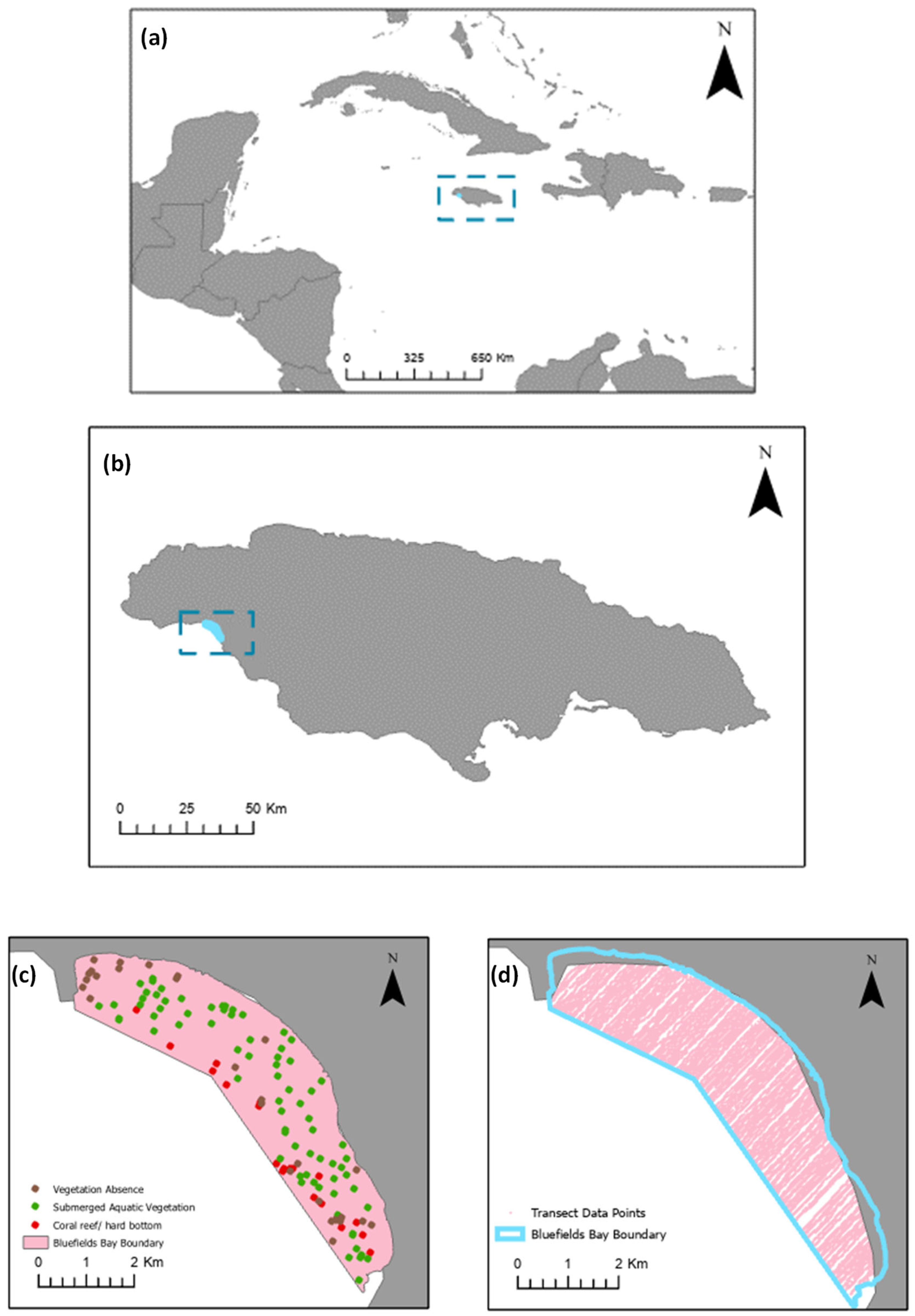
2.1. Study Site

The study area is the Bluefields Bay Special Fish Conservation Area (BBSFCA) (18°10′02″N, 78°02′02″W). It is an MPA that was established on 28 July 2009, and it is found on the southwest coast of Jamaica in the parish of Westmoreland, in southwestern Jamaica (Figure 1a,b). It is 13.82 km² in size [30] and a large percentage of the shoreline/intertidal zone comprises mangrove stands (41.7%), followed by sandy beach (35.5%), and the remaining shoreline consists of naturally occurring limestone bedrock and cliffs or manmade structures including rip rap, sea walls, and boulder/rubble (22.8%) [35]. The predominant benthic features in the bay include seagrass beds dominated by Thalassia testudinum and a smaller area dominated by Halodule wrightii, unconsolidated bare sediment with sparse algal cover, including Halimeda sp., unconsolidated bare sediment, and coral reef [30]. There were three hurricanes that may have affected Bluefields Bay during the study period. These included Hurricanes Gilbert, Ivan, and Dean. Hurricane Gilbert made landfall on 12 September 1988, and had an average windspeed of 204–213 km h⁻¹. Hurricanes Ivan and Dean passed at a distance of 40.3 km and 40.9 km, respectively, from the eyes of the two hurricanes to the closest point along the southern coastline of Jamaica on 11 September 2004, and 20 August 2007, respectively, and had an average windspeed of 241–250 km hr⁻¹ and 231 km h⁻¹, respectively [36] (Figure A4).

2.2. Satellite Imagery

In total, 27 satellite images of the study site from 1984 to 2021 (37 years) were downloaded from the United States Geological Survey (USGS) website (https://earthexplorer.usgs.gov/; accessed on 12 February 2023) (

Table A1. List of Landsat satellite images that were used in this study.

Name of File	Landsat Series	Path	Row	Date
LT05_L2SP_012047_19841009_20200918_02_T1	Landsat 4–5	12	47	9 October 1984
LT05_L2SP_012047_19850302_20200918_02_T1	Landsat 4–5	12	47	2 March 1985
LT05_L2SP_012047_19860217_20200918_02_T1	Landsat 4–5	12	47	17 February 1986
LT05_L2SP_012047_19870628_20201014_02_T1	Landsat 4–5	12	47	28 June 1987
LT04_L2SP_012047_19880926_20200917_02_T1	Landsat 4–5	12	47	26 September 1988
LT05_L2SP_012047_19900503_20200915_02_T1	Landsat 4–5	12	47	3 May 1990
LT04_L2SP_012047_19930111_20200914_02_T1	Landsat 4–5	12	47	11 January 1993
LT05_L2SP_012047_19940223_20200913_02_T1	Landsat 4–5	12	47	23 February 1994
LT05_L2SP_012047_19950330_20200912_02_T1	Landsat 4–5	12	47	30 March 1995
LT05_L2SP_012047_19960316_20200911_02_T1	Landsat 4–5	12	47	16 March 1996
LT05_L2SP_012047_19970404_20200910_02_T1	Landsat 4–5	12	47	4 April 1997
LT05_L2SP_012047_19991019_20200907_02_T1	Landsat 4–5	12	47	19 October 1999
LE07_L2SP_012047_20000131_20200918_02_T1	Landsat 4–5	12	47	31 January 2000
LE07_L2SP_012047_20021120_20200916_02_T1	Landsat 7	12	47	20 November 2002
LE07_L2SP_012047_20060304_20200914_02_T1	Landsat 7	12	47	4 March 2006
LE07_L2SP_012047_20060421_20200914_02_T1	Landsat 7	12	47	21 April 2006
LT05_L2SP_012047_20080520_20200829_02_T1	Landsat 4–5	12	47	20 May 2008
LT05_L2SP_012047_20100118_20200825_02_T1	Landsat 4–5	12	47	18 January 2010
LE07_L2SP_012048_20130510_20200907_02_T1	Landsat 7	12	48	10 May 2013
LE07_L2SP_012047_20131017_20200907_02_T1	Landsat 7	12	47	17 October 2013
LC08_L2SP_012047_20131126_20200912_02_T1	Landsat 8	12	47	26 November 2013
LC08_L2SP_012047_20150116_20200910_02_T1	Landsat 8	12	47	16 January 2015
LC08_L2SP_012047_20160220_20200907_02_T1	Landsat 8	12	47	20 February 2016
LC08_L2SP_012047_20170222_20200905_02_T1	Landsat 8	12	47	22 February 2017
LC08_L2SP_012047_20190111_20200830_02_T1	Landsat 8	12	47	11 January 2019
LC08_L2SP_012048_20200318_20200822_02_T1	Landsat 8	12	48	18 March 2020
LC08_L2SP_012047_20210422_20210430_02_T1	Landsat 8	12	47	22 April 2021

). We only chose images with no turbidity. Also, we tried as much as possible to include images that were collected during the same time of the year, corresponding to the first (January–mid-April) or the second dry season (July to August) to ensure consistency, but several images used were collected during the major rainy season (September–December). Nevertheless, comparisons between and among images from different years can be improved if the atmospheric conditions at the time when the images were captured are accounted for or removed. As such, Landsat Collection 2 Level 2 images, derived from an atmospherically corrected surface reflectance image product, were downloaded and used. The image bands were stacked and reprojected to the local datum, JAD 2001. The 2006 and 2013 Landsat 7 images had missing data (SLC off) and therefore, the mosaic function in ArcGIS Pro (2.5.1) was used to merge two 2006 and 2013 images that were collected three and five months apart (see Table A1), respectively, to fill in the gap of these missing data.

2.3. Hydroacoustic Auxiliary Data

Processed hydroacoustic survey data from [30,35] were used in this study. The hydroacoustic survey was conducted during the period July 26–2 August 2013 and the data were collected using a 206 kHz Biosonics DT-X split-beam side-mounted transducer [30]. The transducer had a beam width of 7°, which approximated to a footprint size of 0.01 to 0.05 m² at a depth of 1–2 m [30] and it was multiplexed to allow for simultaneous sampling of macrophytes (0.4 m/s pulse duration) and other benthic features [30]. During the survey, horizontal positioning data (±0.30 m) were obtained from a Fugro Starfix HP Differential GPS and the survey was conducted along predefined transect tracks with 50 m spacings, covering 294.178 km [30] (Figure 1d). The hydroacoustic data were processed using two software packages: Visual Bottom Typer (VBT_TM, Version 1.12; Biosonics Inc., Seattle, WA, USA), which was used to derive depth values that were spatially referenced and were subsequently corrected for tidal differences and reprojected to the local datum, and EcoSAV^TM (v1.0, Biosonics Inc., Seattle, WA, USA), which was used to derive percentage seagrass or submerged aquatic vegetation (SAV) cover data that were also spatially referenced [30].

The spatially referenced, reprojected, and tide-corrected depth data points were interpolated using universal kriging to create a bathymetric surface model (BSM) [30], from which a bathymetric position index (BPI) and a rugosity map were created. The BPI map was created after applying the “Land Facet Corridor Designer Tools” for ArcGIS 10 [37] to the BSM layer [31]. The BPI map data have continuous values that change from negative to positive; this represents a transition from valleys to slopes and then to ridge tops. “Block Statistics” was used to create the rugosity map in ArcGIS 10.6 [31]. Grey Level Co-Occurrence Matrix (GLCM) maps were generated in the R programming language environment versions 4.2.1 and 4.3.1 [38,39] using the “glcm” package [40]. The package was used to calculate texture statistics (mean and variance) derived from grey-level co-occurrence matrices (GLCMs) for bands 1, 2, and 3 for Landsat 4–5 and 7 images, and bands 1, 2, 3, and 4 for Landsat 8 images. Specifically, average GLCM textures in all directions were calculated using shifts of 45 degrees for the image bands, and these were outputted as maps of mean and variance GLCM textural measures.

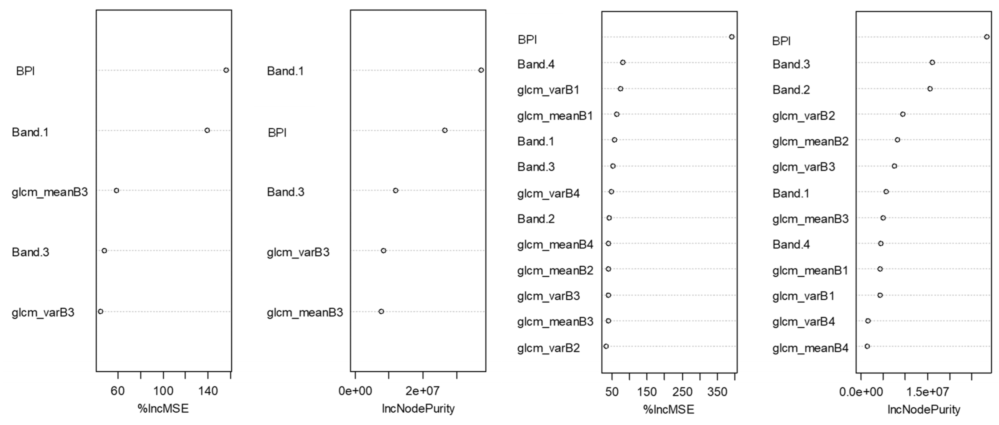
2.4. Random Forest Models and Model Validation

SAV percentage cover maps were produced by integrating the spatially referenced SAV data with Landsat image reflectance data and auxiliary data using random forest regression (RFr) models following [31]. Before the SAV maps were produced, the SAV data were split into training (78% or 107,076 data points) and validation (12% or 14,853 data points) data. The validation data/transects were evenly distributed across the bay. They were selected using a random start, with every tenth data point transect selected and used as a validation transect (16 transects in total), together with transects running perpendicular to the shoreline (4 in total) [30,35]. Additionally, before the RFr models were built, the coordinates of the track points of the SAV percentage cover data were generated. These were used to extract data from maps of the auxiliary data (BSM [depth] and BPI) and band reflectance and GLCM mean and variance data from the images for the year 2013 (bands 1–3 for the composite Landsat 7 image with the missing data filled in and bands 1–4 for Landsat 8 image). Images from the year 2013 were used because the hydroacoustic survey was conducted during this time. Two RFr models were built using the “randomForest” package [41] in R, both of which included SAV percentage cover data at each track point as the dependent variable and BSM and BPI as predictors. One of the two models included the extracted 2013 composite Landsat 7 band reflectance and GLCM data as additional predictors, and the other RFr model included the 2013 Landsat 8 band reflectance and GLCM data as additional predictors. After each model was built and run, the predicted SAV cover at each validation data point was generated by the models. These were then compared to the observed SAV cover at each validation data point, and the following validation criteria were generated: mean absolute percentage error (MAPE), root mean squared error (RMSE), mean absolute error (MAE), mean squared error (MSE), bias (a measure of consistent under- or over-forecasting; BIAS), relative bias (rBIAS), and relative mean separation (rMSEP). See [42] for the formulations. Small values of MSE, RMSE, MAE, rBIAS, and rMSEP (lower values or values close to zero) imply that the model is suitable for making predictions, robust, and that predicted values are very similar to observed values. Also, for the MAPE, values close to 0 represent the most accurate predictions; however, all values of MAPE below 100% represent accurate predictions.

Following validation, the most accurate model was then chosen. For the Landsat 8 model, this included all the predictors, whereas for the Landsat 7 model, this included the top 5 predictors (Figure A1;

Table A2. Measures of accuracy calculated for two random forest regression models (RFr) that were used to model the relationship between hydroacoustic submerged aquatic vegetation (SAV) percentage cover data and several predictors including bathymetric position index [BPI] data and band reflectance and Grey Level Co-Occurrence Matrix (GLCM) mean and variance data from Landsat images for the year 2013, for bands 1 and 3 from a composite Landsat 7 image with the missing data filled in and bands 1–4 for a Landsat 8 image. The testing data accounted for 12% of the SAV data or 14,853 data points. Accuracy measures include mean squared error (MSE), root mean square error (RMSE), mean absolute error (MAE), mean absolute percentage error (MAPE), bias (BIAS), relative bias (rBIAS), and relative mean separation (rMSEP). Var (%) = percentage variance explained by the model.

RFr Models	Var (%)	MSE	RMSE	MAE	MAPE	BIAS	rBIAS	rMSEP
SAV × BPI + Landsat 7 reflectance and GLCM data	62.7	656.5	25.6	19.2	39.1	1.3	0.0202	0.4
SAV × BPI + Landsat 8 reflectance and GLCM data	69.8	595.2	24.4	17.7	37.7	0.1	0.0008	0.4

). A polygon shapefile of the BBSFCA was converted to a 2 m gridded raster, and then to a point shapefile. These data points were used to extract data from the auxiliary maps and reflectance and GLCM mean and variance maps for the Landsat 4–5, 7 (1984–2010), and 8 (2015–2021) images and for the 2013 images used for modelling. The RFr model for each Landsat series was then used to predict SAV cover at each point of the point grid for each year of a particular Landsat series using the predictors extracted for each point. For example, the Landsat 7 RFr model was used to predict SAV cover using reflectance data from Landsat 4–5 and 7 images plus the auxiliary data. Similarly, the Landsat 8 RFr model was used to predict SAV cover using reflectance data from Landsat 8 images plus the auxiliary data. No Landsat 4–5 images could be found close to the year of the hydroacoustic assessment (the closest was 2011). Moreover, the wavelength intervals/bandwidth for the Landsat 7 bands were the same as the Landsat 4–5 bands; therefore, the Landsat 7 RFr model was used to predict SAV coverage using Landsat 4–5 image data. The predictions were exported as a 2 m gridded raster, and a single SAV percentage cover map was produced for each year (24 maps in total).

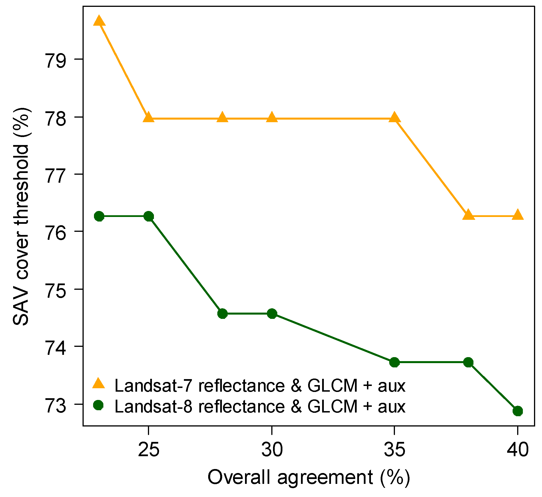
2.5. Benthic Habitat Maps and Accuracy Assessments

Several binary maps for each of the percentage cover maps generated using the 2013 Landsat 7 and 8 series image data were created using different threshold values in raster calculator in ArcGIS Pro 3.0.1. The thresholds used were 23%, 25% 28%, 30%, 35%, 38%, and 40% for the 2013 Landsat 7 and 8 derived SAV percentage cover maps. Values above these thresholds would be used to map SAV presence. The range of values used was previously found to generate the most accurate binary maps [31]. The binary maps created were added to a coral reef map that was generated using a threshold of 0.23 for the rugosity map, also in raster calculator (following [31]). From this, maps with three classes, SAV present, SAV absent, and coral reef, were produced for the maps derived from the two datasets. A total of 118 accuracy assessment (AA) reference data points (21, 23, and 74 for coral reef, vegetation absent, and vegetation present points, respectively), collected by [30] in 2013 at randomly determined points using georeferenced videos/video camera drops (Figure 1), were used to identify the most accurate threshold for each map. The map classes at each AA location were first determined by using the AA points to extract information from the maps on the classes found at each location. An accuracy assessment was then conducted in R using the “asbio” package [43] using the extracted classes and reference data for each map. The most accurate threshold with the highest overall agreement (OA) was identified (following [31]) for the two series (Figure A3). However, we chose the threshold with the second highest OA for the Landsat 4–5 and 7 maps and used it to generate a benthic habitat map for each year during the period 1984–2010 (30% SAV cover threshold) and we used the second of two thresholds with the highest OA for the Landsat 8 maps to create maps for the period 2013–2021 (25% SAV cover threshold). These thresholds were chosen because they consistently produced maps that closely matched (visually) the unclassified images.

2.6. Assessment of Landscape Scale Change and Predictors of Change in SAV Cover and Area over Time

Mean SAV percentage cover and SAV total area for each year for the entire bay were determined and used to assess changes over time and the possible effects of rainfall on SAV percentage cover and area. Additionally, monthly rainfall data for the site (Bluefields Bay) for the period 1901 to 1994 were obtained from the Jamaican Meteorological Service. This dataset did not cover the entire period of this study and as such, this was supplemented using monthly rainfall data from Savanna-la-Mar, the capital of the parish of Westmoreland, which is located ≈ 5.6 km away. A generalized additive mixed model (GAMM) with an autoregressive moving average (ARMA) error structure (used to account for temporal autocorrelation) and a cubic smoothing spline was used to determine if there was a significant trend in total annual rainfall over time. For this assessment, only years that included data for all months were used. A GAMM was also used to determine if there were significant changes/trends in SAV percentage and SAV total area over the period 1984–2021. The GAMM was implemented using the “mgcv” package [44,45,46,47]. The ARMA error structure was defined by two parameters: the number of autoregressive (AR) (p), and the number of moving average (MA) parameters (q) [48]. The autoarima function from the “forecast” package [49,50] was first used to determine the most suitable number of ARMA parameters based on AIC, AICc (AIC corrected for finite sample sizes), and BIC (Bayesian information criterion) values. It was applied to the residuals from a generalized additive model (GAM) that included the dependent and independent variables with no ARMA error structure. The ARMA values obtained from the GAM using the autoarima function were used in the GAMM. Before final models were accepted, the autocorrelation and partial autocorrelation functions (ACF and PACF, respectively) were used to check the residuals (normalized for the GAMM) of the models to determine if they were white noise (random and not autocorrelated). Additionally, the model parameters (GAMM) and the 95% confidence intervals of the AR and MA were checked to ensure that they did not include zero. This indicated that there were no problems with the error structure and the model contained an adequate number of explanatory variables. A generalized linear regression (GLM) with a Gaussian link function, implemented using the “lme4” package [51], was used to determine if there was a relationship between monthly SAV percentage cover and area change, and average monthly rainfall. Monthly values were determined using the number of months between the dates when two consecutive Landsat images were recorded. For example, for the 1984 (9 October 1984) and 1985 (2 March 1985) images, the number of months between the two dates was determined (4.8), and the total rainfall, the change in percentage SAV cover, and the change in total area of SAV between the two dates were divided by the number of months. This was repeated for the other image dates. The R-squared values for the GLMs were generated using the “MuMIn” package [51].

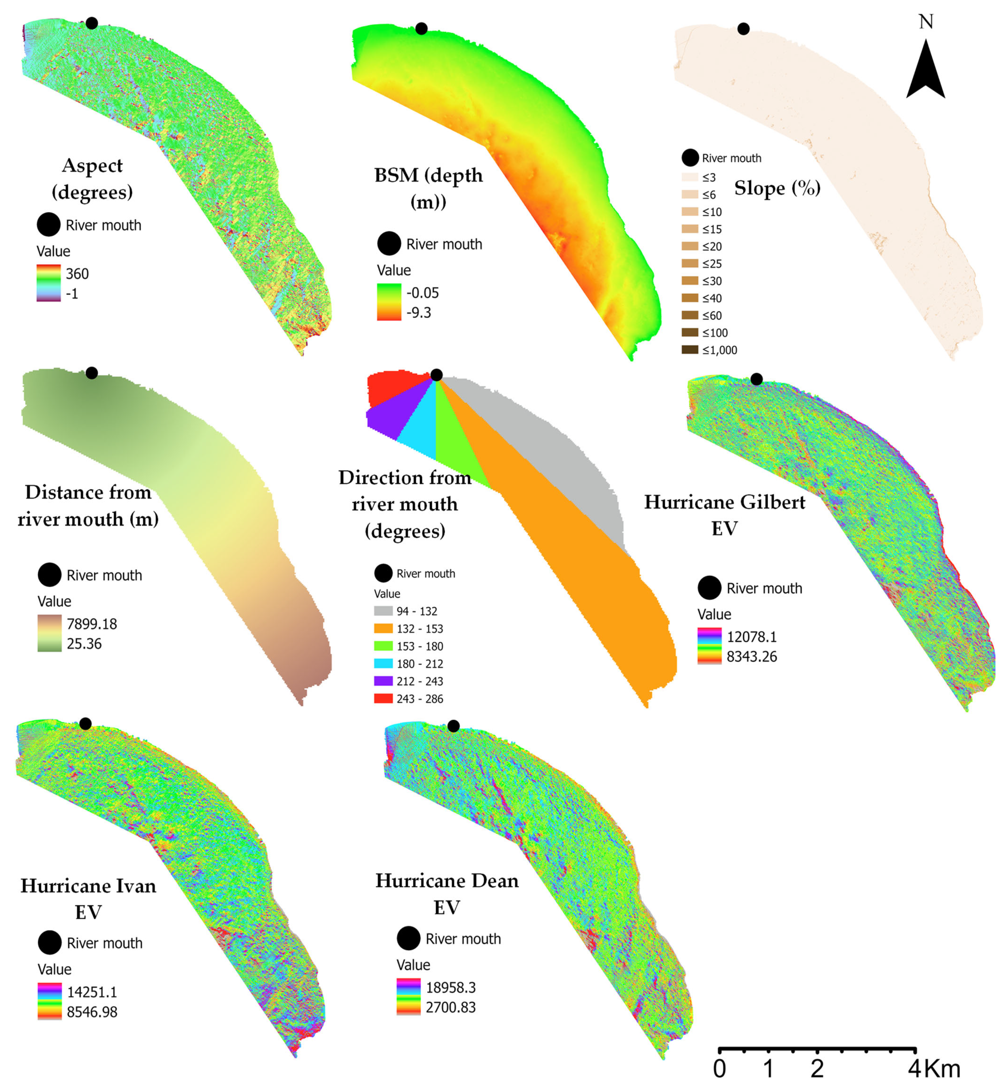
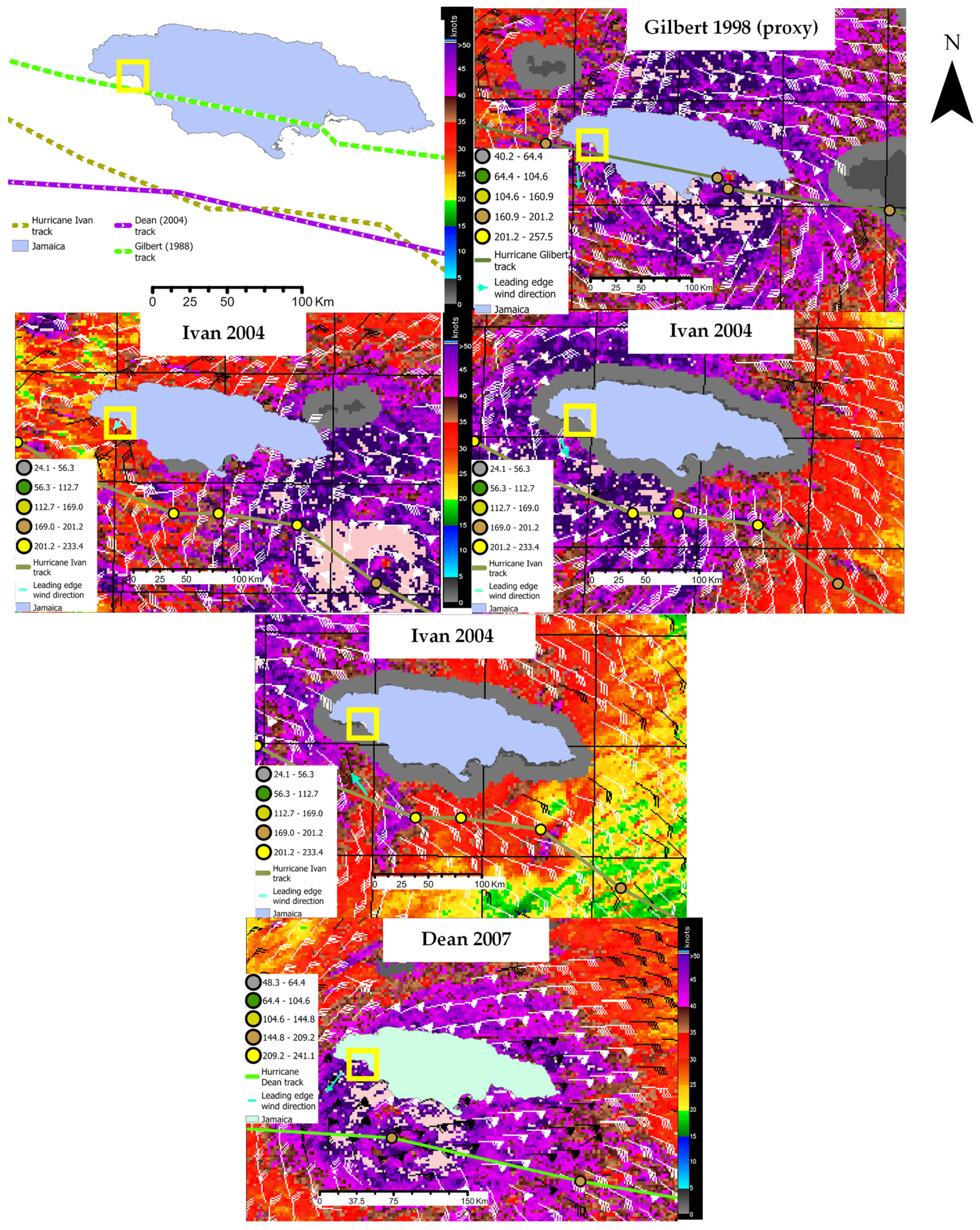
2.7. The Spatial Pattern Predictors of SAV Change

Pixel-based regressions were used to assess the effects of rainfall on the spatial pattern of SAV loss and gain and changes in percentage cover over the period 1984–2021. First, maps of binary (1 for loss or gain and 0 for no change) and percentage cover change were generated by subtracting one image year from the subsequent year. A total of 23 maps for each category of assessment, that is, binary loss, gain, and percentage cover change, were therefore produced. A logistic GLM implemented using the “lme4” package with a quasibinomial distribution (to account for under- or over-dispersion) and a logit link function was then used to model the relationship between the binary map values (1 or 0) at each pixel and total monthly rainfall. The relationship between the percentage cover change per month map values (change divided by the time (months) between consecutive maps) at each pixel and rainfall was modelled using a linear regression. The outputs from the regressions, particularly the marginal (for the logistic GLM) or adjusted (for the linear regression) R-squared, gradient estimate, and p-value at each pixel, were represented as maps. These maps highlighted locations on the ground that were directly influenced by rainfall positively or negatively over the study period.

We then assessed the influence of proxies to rainfall, that is, proximity/Euclidian distance and cardinal direction from the mouth of the main river that empties into the bay, and other possible predictors such as topographic features, including aspect and slope, and depth and exposure to past hurricanes or exposure vulnerability (EV) (Figure A3), on the spatial patterns of SAV loss, gain, and percent cover change between successive time periods (i.e., 1984–1985, 1985–1986, etc.). EV is a unitless measure that has been previously used to link the heterogeneity of hurricane exposure to responses shown by terrestrial vegetation at sites that experienced hurricane disturbance [52]. Although EV maps have primarily been used and validated in a terrestrial context, they were used in this study to determine if they can also explain changes in SAV cover and extent due to damage caused by/changes induced by hurricanes (to seagrass beds) in a nearshore marine environment. For this assessment, EV maps were generated following the method outlined in [36,52] and in the Supplementary Material. A single EV map of each hurricane was generated (Figure A3), and additionally, the EV maps for Ivan and Dean were averaged. Average EV of multiple hurricanes can also be an important predictor of vegetation response over time when two or more hurricanes impacted a site [36,52].

2.8. Hierarchical Bayesian Modelling Framework Used to Identify Spatial Pattern Predictors of SAV Change

The SAV loss, gain, and percent cover change maps were converted to point shapefiles, appended with the X and Y coordinates at each point, and used to extract values of the predictors at each point. The relationship between SAV loss, gain, and percent cover change and the predictors at each point for successive years was then evaluated. These datasets were large and spatially autocorrelated, and there are very few methods that can efficiently handle such datasets. As such, we used a Bayesian approach based on the Integrated Nested Laplace Approximation (INLA), implemented using the ‘INLA’ package [53,54,55,56,57] due to its flexibility and ability to efficiently handle large spatial data [55,58]. We developed Hierarchical Bayesian models with a spatial random effect that were formulated according to a spatially explicit generalized linear mixed model (GLMM) framework. Therefore, the response variable at each successive period or overall and plot location was assumed to follow a distribution from an exponential family. Consequently, appropriate distributions and link functions were chosen for the response variables such as a zero-inflated binomial Type 1 (ZIB.1) or a binomial (if the model failed to converge) distribution with a logit link function for the binary loss and gain data and a Gaussian distribution for the percentage change data. The chosen exponential family parameters (ø) were linked to a structured additive predictor η by their link function g(·), so that g(ø) = η and the linear predictor was defined as:

η = β₀ + β₁ × a + β₂ × b + f(s),

where η was the linear predictor for the response variables, β₀ was the intercept, and β₁ and β₂ were the (linear) regression coefficients for the predictors a and b. The random effect (spatial) was introduced using the semiparametric function f(·) [55]. f(s) represented a spatially structured (s) random effect. The spatial location of each transect point (the X, Y coordinates) was used as the basis of the spatial random effect. The Stochastic Partial Differential Equation (SPDE) approach of [54] was used to model the spatially structured random effect as a Gaussian random field (GRF). The SPDE method subdivides the domain or the area of interest into non-intersecting triangles, creating an index mesh instead of a regular grid [54]. Linear combinations of basis functions, defined on the locations of the set of vertices, are used in triangulation process [54]. Please see [54] for a more detailed explanation of the SPDE approach. In this study, the area of the MPA was used as the domain to approximate the spatial fields. To reduce boundary effects (where the variance is twice as large as inside the domain), the mesh did not extend beyond the study area.

The default and recommended priors, that is, vague priors or estimations of non-informative priors [59], were used to develop the models. Additionally, the penalized complexity prior (PC-prior) framework of [60] was adopted to remove or avoid overfitting, particularly for the spatially structured effect, which was found to be operating at a smaller (but neither at a similar nor higher) spatial scale than the covariates or predictors of the models [61]. When this occurred, the spatial effect explained the data better than the covariates and the model was meaningless [61]. Additionally, model accuracy and the marginal R-squared were inflated, while the Deviance Information Criterion (DIC) was deflated, and as a result, they could not be used for model selection. To correct this, a weakly informative PC-prior derived by [60] was used to define the model parameters for the SPDE model as the practical range and the marginal standard deviation. The PC-prior penalized complexity by shrinking the range to infinity and the marginal variance to zero [60]. Several values for the range were used (starting with half the distance between the furthest points), until there was no overfitting.

Before the statistical tests were performed, the Spearman’s rho statistic and test were used to identify significantly correlated independent variables (with a correlation of >0.55). Additionally, a Deviance Information Criterion (DIC) computed in R-INLA, which is analogous to the Akaike Information Criterion (AIC) but it is more suitable for hierarchical Bayesian models [62], was generated for each model. This was used to compare the goodness-of-fit of the models; specifically, models with the lowest DIC values were generally considered as the best. The marginal R-squared (following [63]) was also used to assess model fit. It was calculated as follows:

$$100 \text{×} (1-({\displaystyle {\sum }_{t=1}^t}{\displaystyle {\sum }_{n=1}^n}(depend-fitted)2/{\displaystyle {\sum }_{t=1}^t}{\displaystyle {\sum }_{n=1}^n}(depend-\mathrm{m}\mathrm{e}\mathrm{a}\mathrm{n}(depend\left)\right)2\left)\right),$$

where t is time when n subjects were considered, depend is the response variable, and fitted represents the values predicted by the model. Model validation was conducted using a k (five)-fold cross-validation using the validation criteria used previously for the Rfr models. A receiver operating characteristic (ROC) curve value (AUC) was calculated for the SAV loss and gain models using the “pROC” package [64] in R and used as an additional measure of model accuracy.

We scaled all our models so that they had a generalized variance equal to 1 and to ensure that the precision parameters for different covariates or intrinsic models were comparable or had the same interpretation [65]. In general, it is usually difficult to identify the ‘best’ parsimonious model, because competing models can often describe the same data just as well [66]. We therefore applied stringent model selection criteria, but we prioritized the use of the validation criteria, and model selection included several steps. We first determined the most suitable type of regression, that is, either a linear or polynomial (and the order of the polynomial) regression, for modelling the relationship between each predictor and the dependent variable. All the orders of a polynomial regression must be important (the Bayesian equivalent to a significant frequentist relationship) before it is accepted if it is found to be more suitable (based on the DIC and marginal R-squared values). The linear form of the predictor was used during model selection if the relationship (linear or polynomial) between the predictor and the dependent variable was not important. All possible combinations of predictors were then evaluated, and we used the DIC and marginal R-squared values to choose the best 2 to 8 models. For the chosen models, all predictors had to be important and uncorrelated (with a correlation coefficient of ≤0.55, and they were not linearly or monotonically correlated). A 5-fold cross-validation was then used to validate the best models and the AUC was calculated for each model. The final parsimonious model, which yielded the most accurate predictions and had uncorrelated predictors at each successive period, was then selected. The final models included the most important predictors for each period, but they may not have had the lowest DIC or the highest marginal R-squared and AUC, as again, model accuracy was prioritized for model selection. In addition to reporting the best model, we reported the top 2 to 8 most accurate parsimonious models and their accuracies (Tables S1–S3).

3. Results

The RFr models used to generate SAV percentage cover maps from the Landsat 4–5 and 7 and the Landsat 8 satellite series data explained 62.7% and 69.8% of the variance in the data and were reasonably accurate, with an MAE of 19.2% and 17.7%, respectively, a very low or marginal bias, and an RMSE of 25.6% and 24.4%, respectively (Table A2). Importantly, the MAPE was less than 100%, indicating that the models were ideal for predicting (Table A2). The most important predictor was BPI, followed by reflectance data for bands 1 and 4 for the Landsat 4–5 and 7 and Landsat 8 series models, respectively (Figure A1). The chosen thresholds had an OA of 78% and 75% for the Landsat 7 and Landsat 8 three class maps, respectively (Figure A2). Map accuracy/uncertainty for the years before and after 2013 was not quantified because it would be difficult to assess past accuracies without in situ reference data for each year. The percentage cover and binary maps with coral reef class added in (benthic feature map) are presented in Figure 2 and Figure 3. Percentage cover varied across the bay over time, with an area close to the mouth of the river consistently having the lowest SAV percentage cover, and this area was largely classified as SAV absent in the benthic features maps, when the thresholds were applied (Figure 2 and Figure 3). For the years 1990, 1999, 2000, 2013, 2015, and 2019, most of the bay (>70%) had a percentage cover of >80% (Figure 2). For 1993, most of the bay had a percentage cover of ≤60%, but generally, for all other years, there was a higher SAV percentage cover found across the bay (up to 80%) (Figure 2). A notable shift in the pattern of SAV presence/absence occurred in 2006, with the area of the SAV absent class around the mouth of the river increasing, and this class was found extensively across the south of the bay for the first time (Figure 3). This change was attributed to the impact of Hurricane Ivan in 2004.

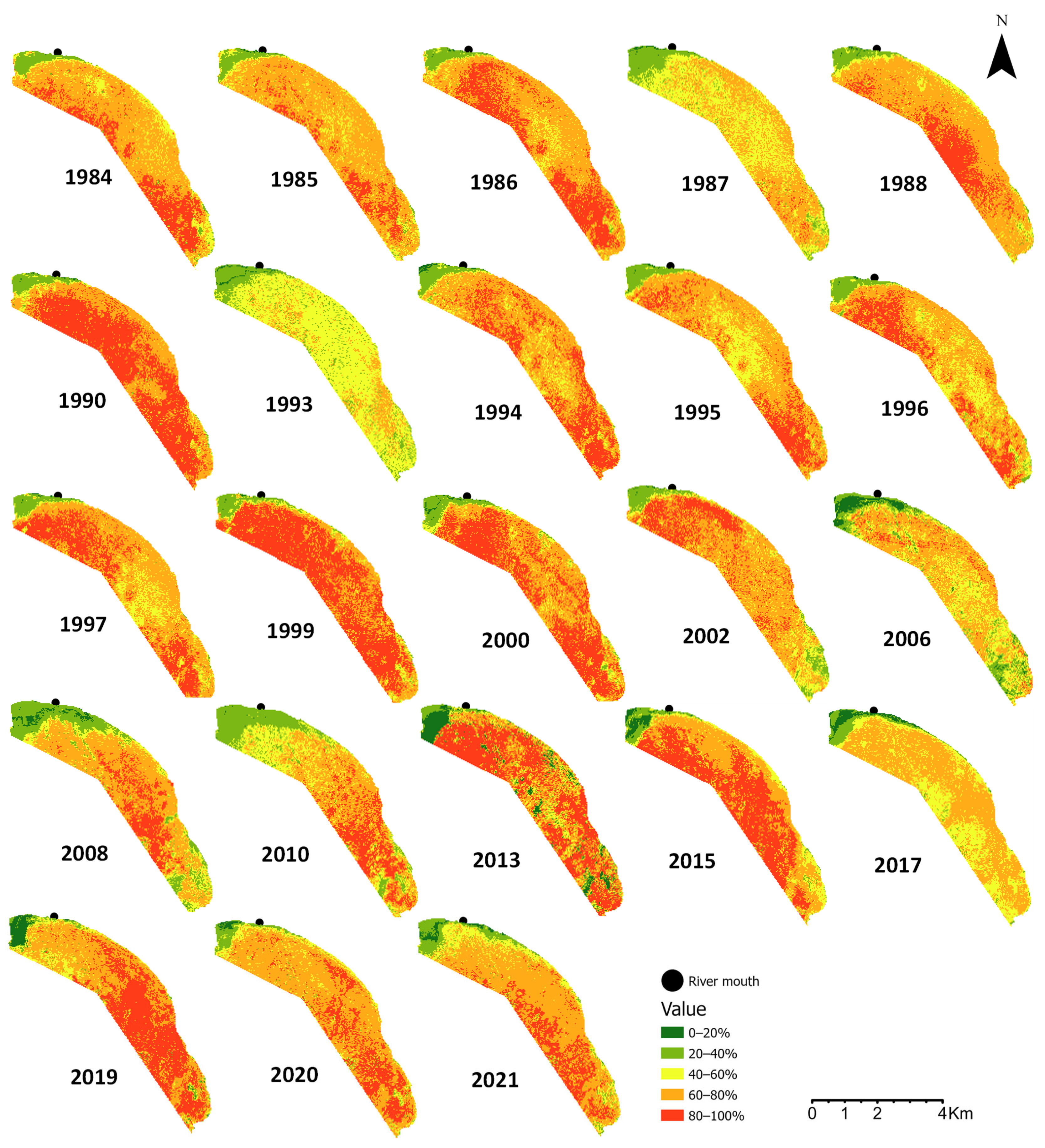
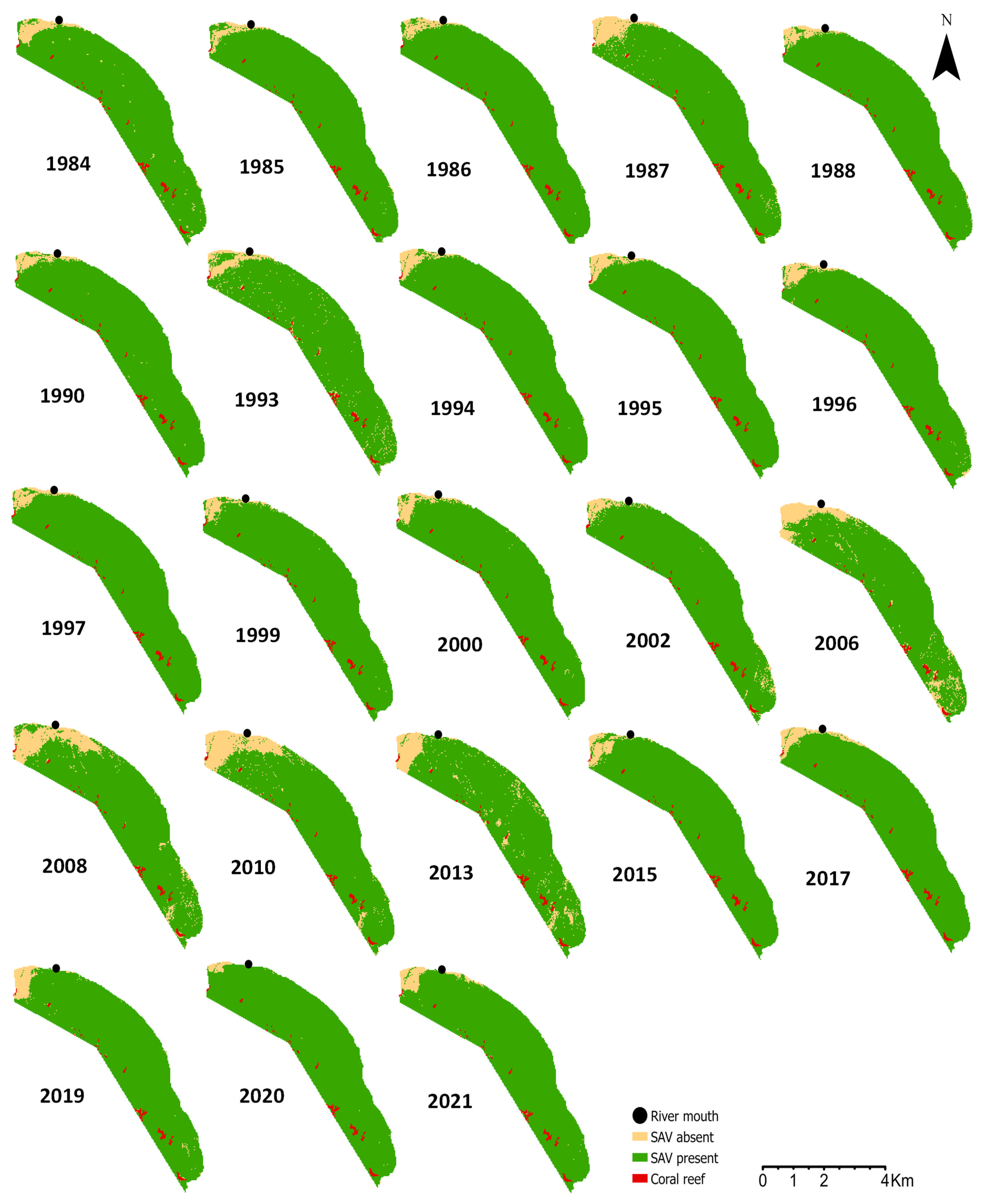
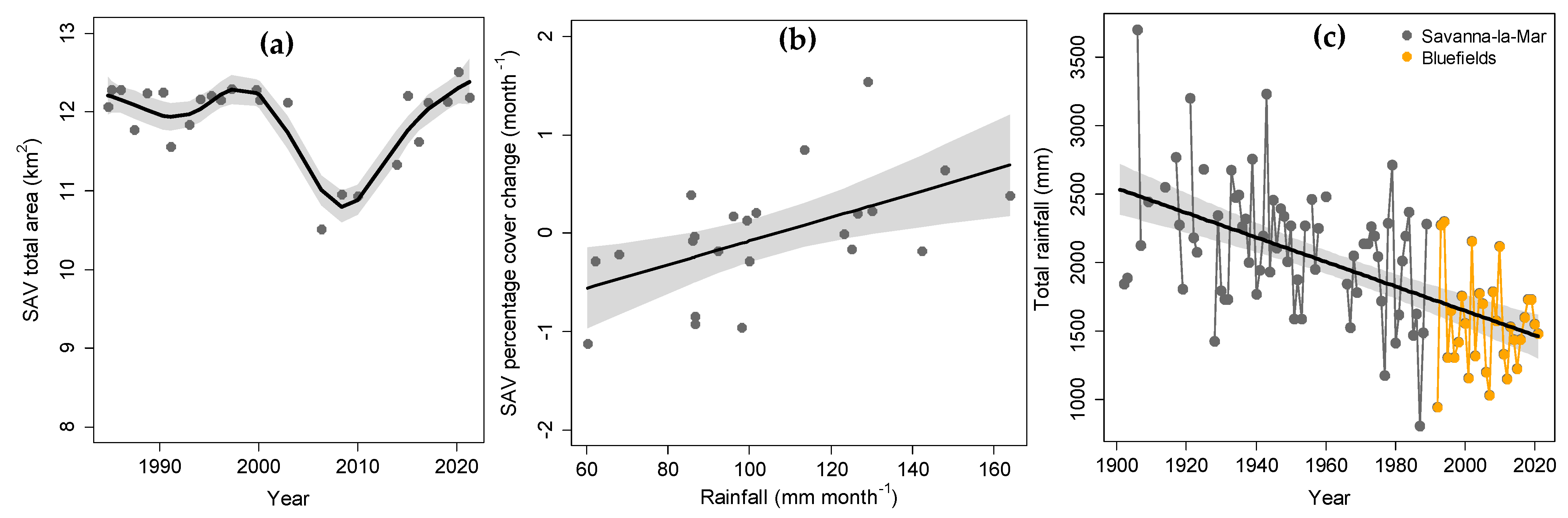
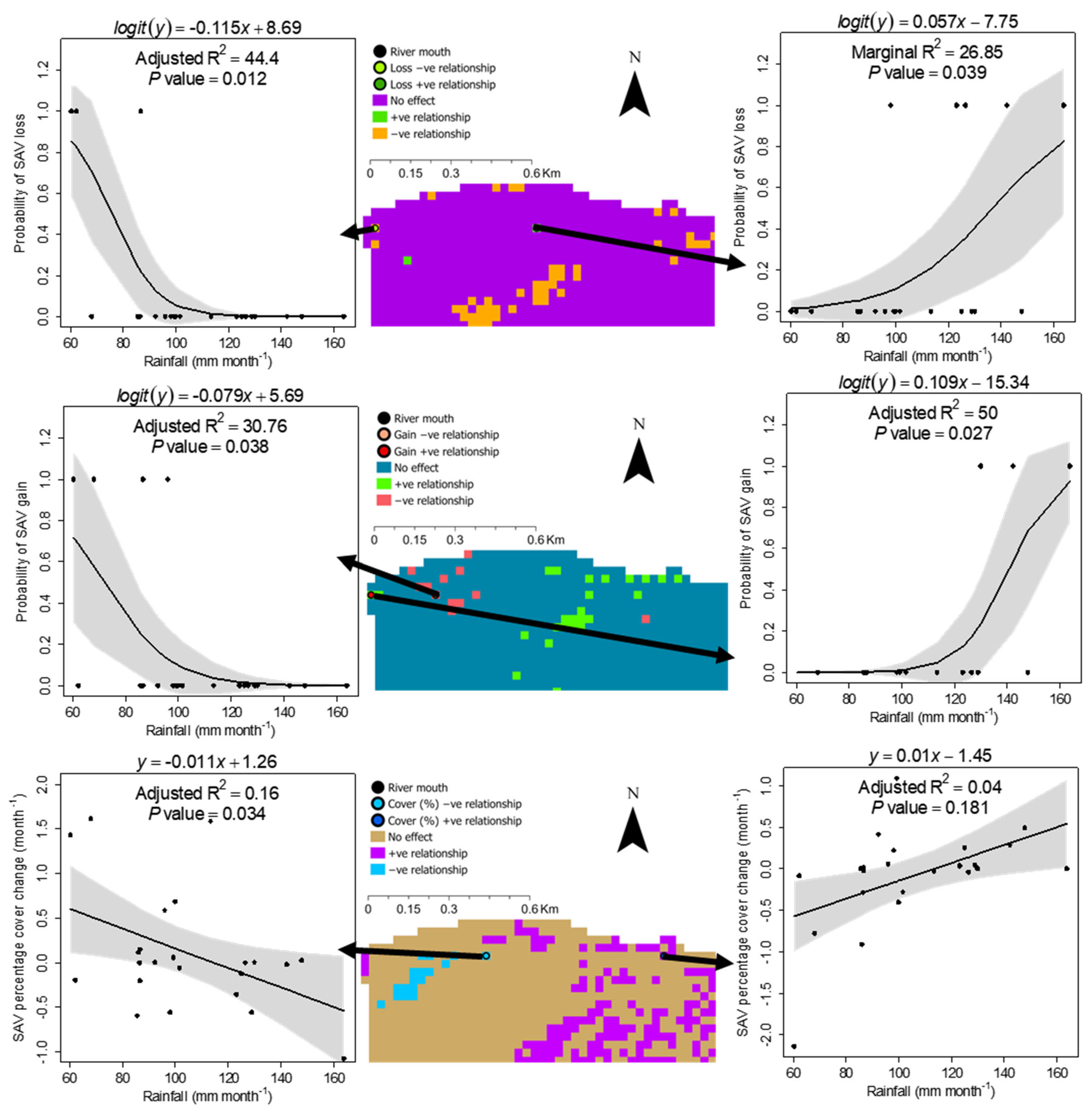
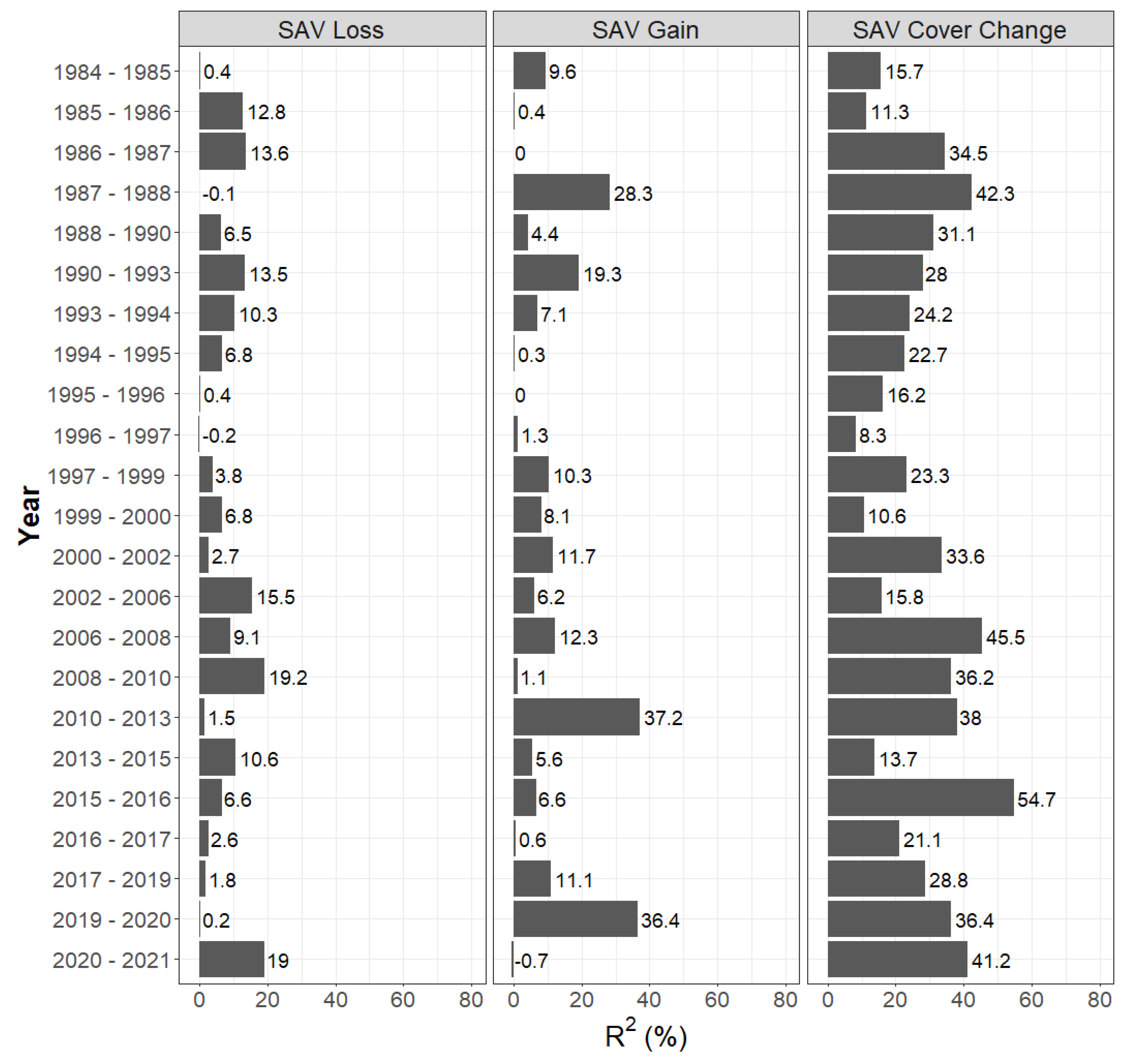
3.1. Landscape Scale Changes and Predictors

The total area of SAV changed significantly over time (

Table 1. Results obtained from a generalized additive model (GAM), a generalized additive mixed model (GAMM) with an autoregressive moving average (ARMA) error structure, and a generalized linear model (GLM) used to assess the trend in total (annual) rainfall over time (1901–2021), the trend in total area of submerged aquatic vegetation (SAV) over the study period (1984–2021), and the relationship between monthly SAV percentage (perc.) cover change and rainfall over the study period, respectively, for Bluefields Bay, Jamaica.

Models and Correlation Structure	Parameter	Value	L 95% CI	U 95% CI	S.E.	t/F	p	Adj. R2/R2
Rainfall (mm) × Year (GAM)	Intercept	1943.6			42.4	45.9	<0.001	34.7%
	s(Year)					50.5 †	<0.001
SAV total area (km2) × Year (GAMM)	Intercept	11.9			0.02	686.5	<0.001	69.5%
ARMA (2, 0)	s(Year)					71.7 †	<0.001
	Phi 1	−0.76	−1.25	−0.26
	Phi 2	−0.43	−0.77	0.02
SAV perc. cover change (month−1)	Intercept	−1.28			0.43	−2.95	0.0077	28.9%
× Rainfall (mm month−1) (GLM)	Rainfall	0.012			0.004	2.99	0.007

L = lower; U = upper; CI = confidence interval; S.E. = standard error; adj. R² = adjusted R²; Phi = autoregressive coefficient; s() = cubic smoothing spline; t = t distribution; F and † = F distribution.

), with a significant reduction in SAV occurring in 2006 (Figure 3 and Figure 4a), which was the largest recorded decline. Recorded loss for the period was 1.62 km², or a 13% decline at a rate of −0.04 km² month⁻¹. Recovery after 2006 was not complete until 2015 (Figure 3 and Figure 4a). The change in extent between 2002 and 2006 coincided with the year when Hurricane Ivan passed by the island (2004) and during the subsequent period (2006–2008), Hurricane Dean passed close by the island (Figure A4). The extent of SAV loss in 2006 occurred over a larger area (Figure 2 and Figure 3), but in general, SAV change (loss and gain) mainly occurred close to the river, as this was an area of active change (Figure 3). Average percentage cover for the entire bay did not change significantly over time, and there were 11 years with an average of >70% percentage cover, with the lowest being 49.8% in 1993. Percentage cover change over successive years was influenced by rainfall (Figure 4b; Table 1), with higher positive percentage cover change occurring when rainfall was higher. Despite the importance of higher rainfall, annual rainfall at the site during the study period was significantly lower than at the start of the 20th century (approximately 1000 mm lower on average), as there was a significant decrease in annual rainfall (Figure 4c; Table 1).

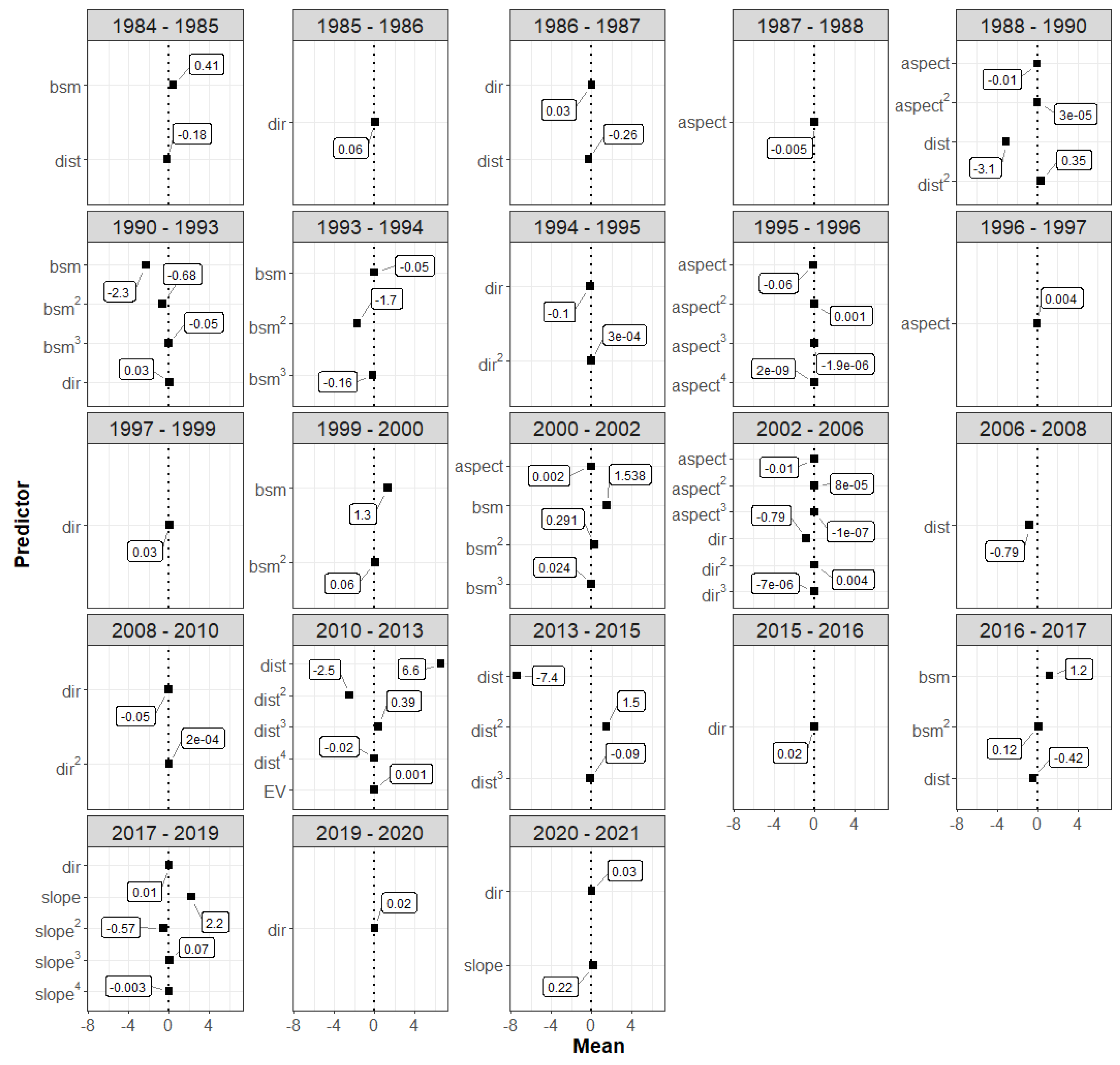
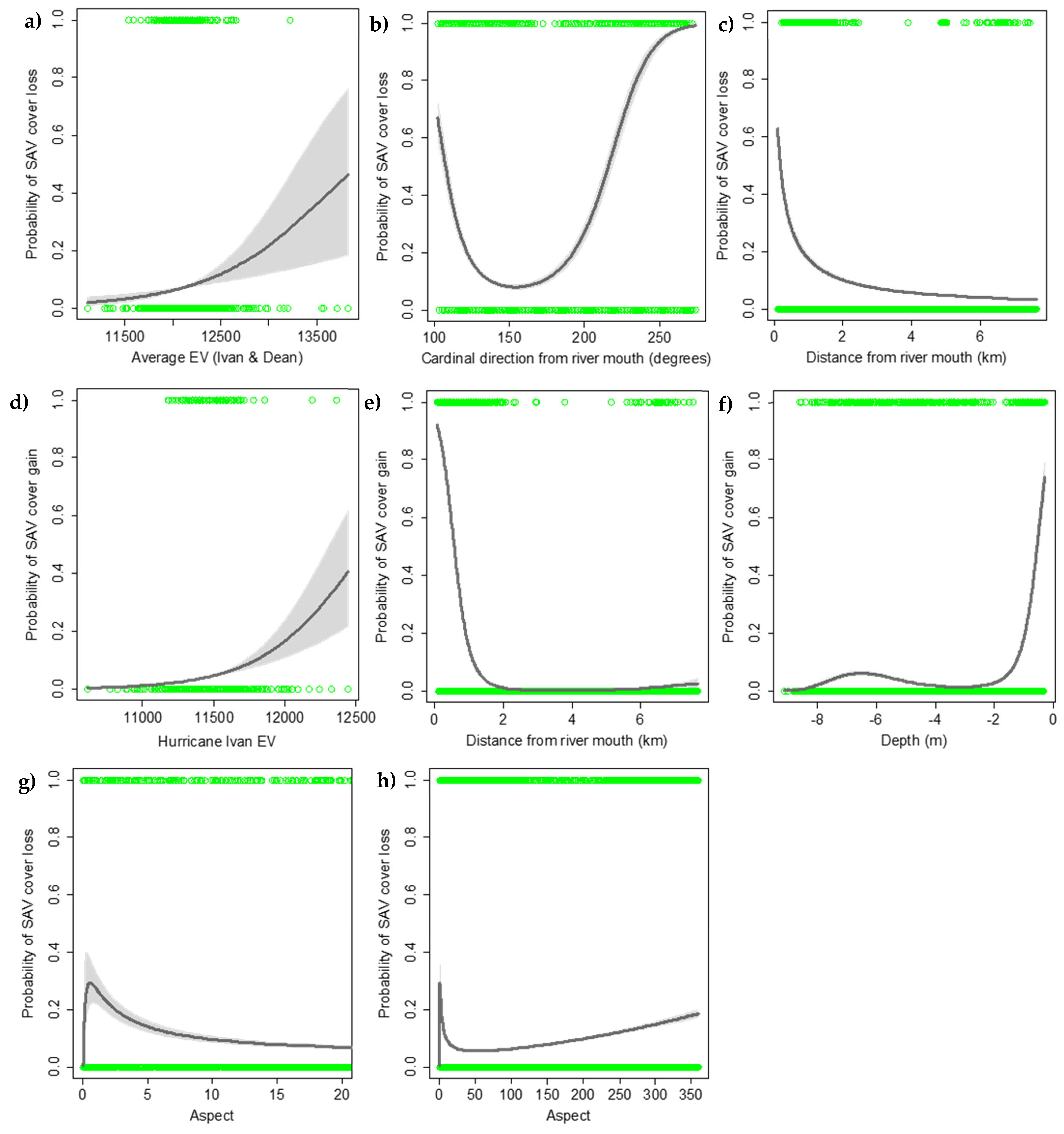
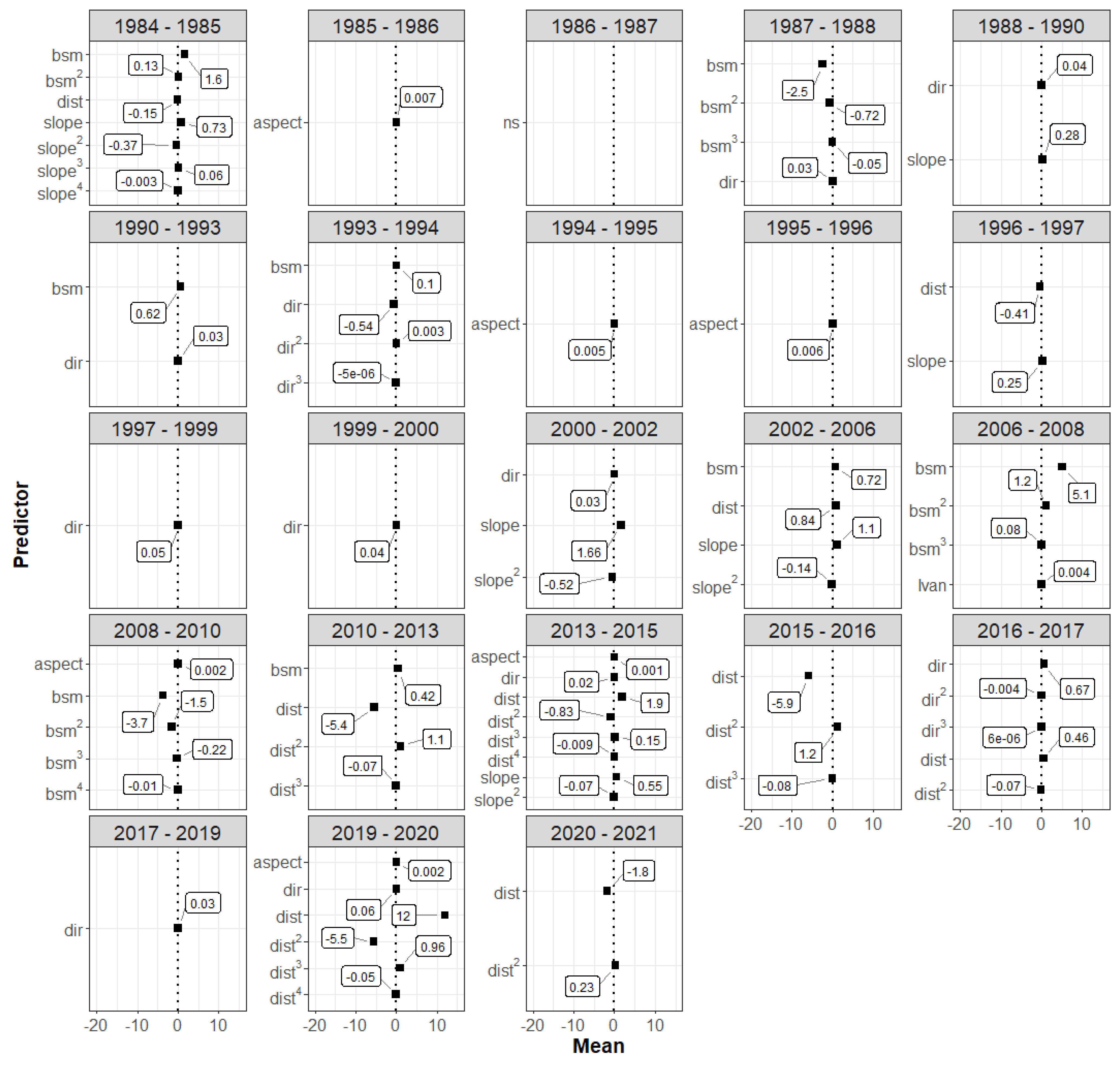
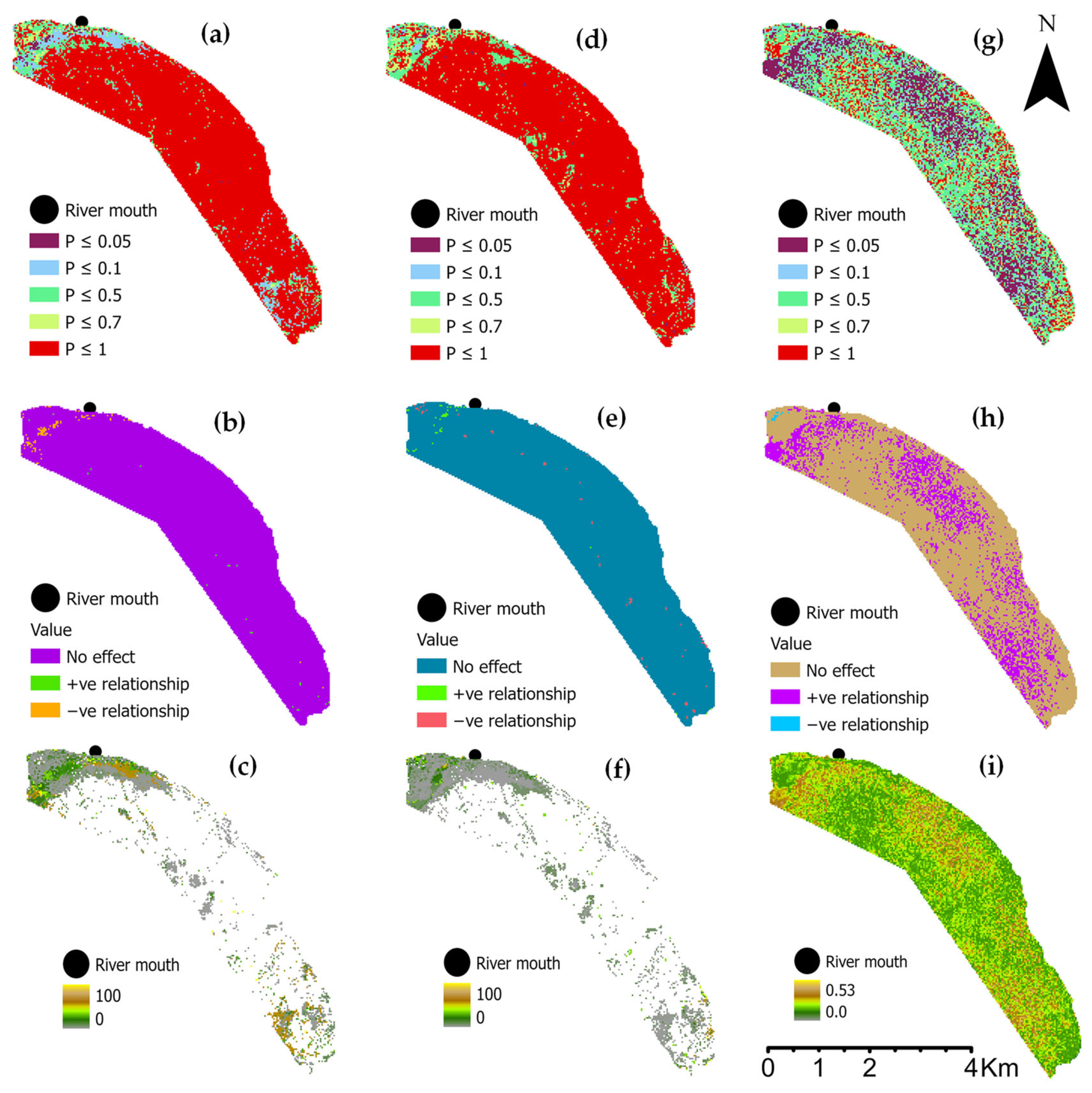
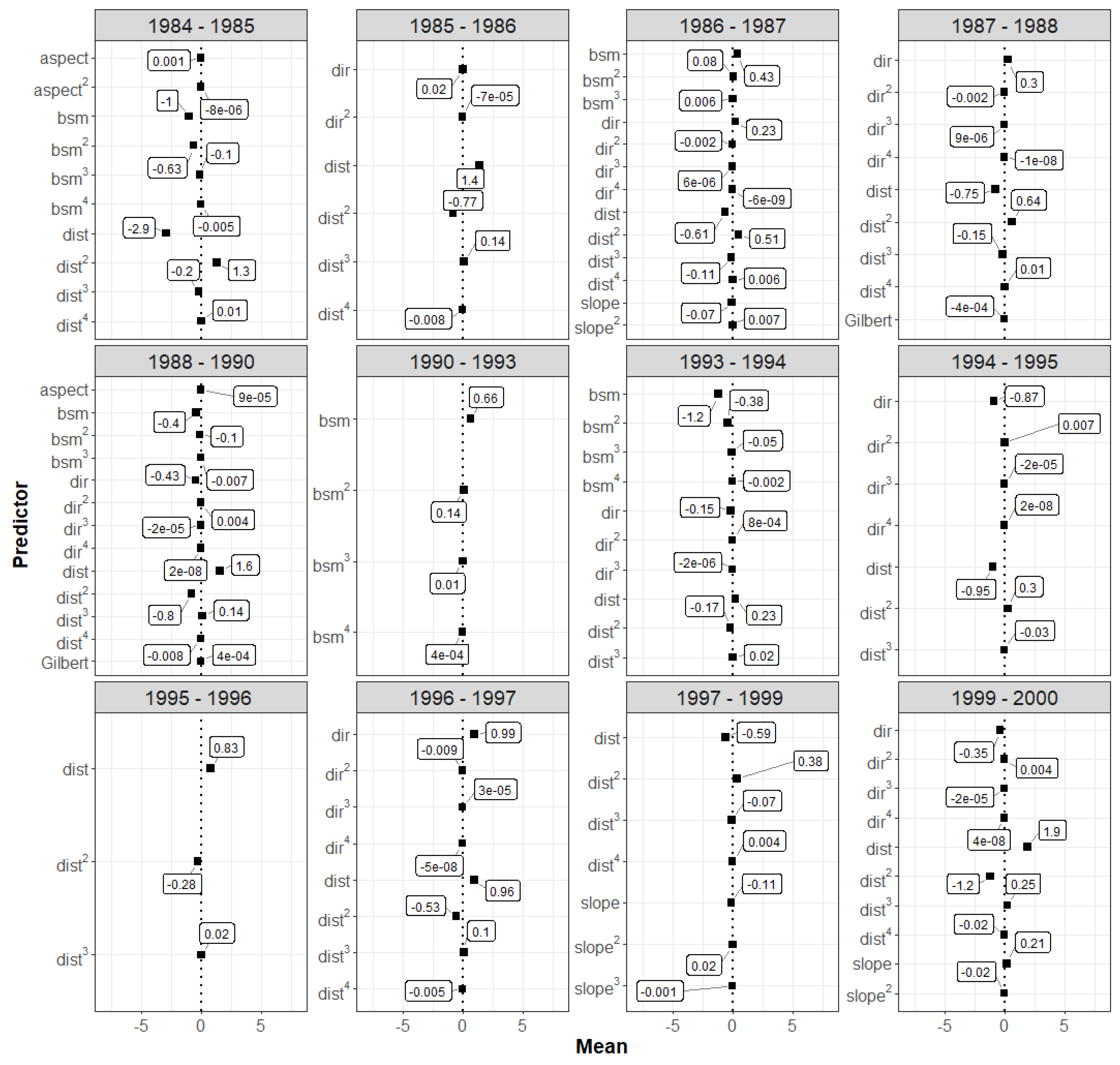
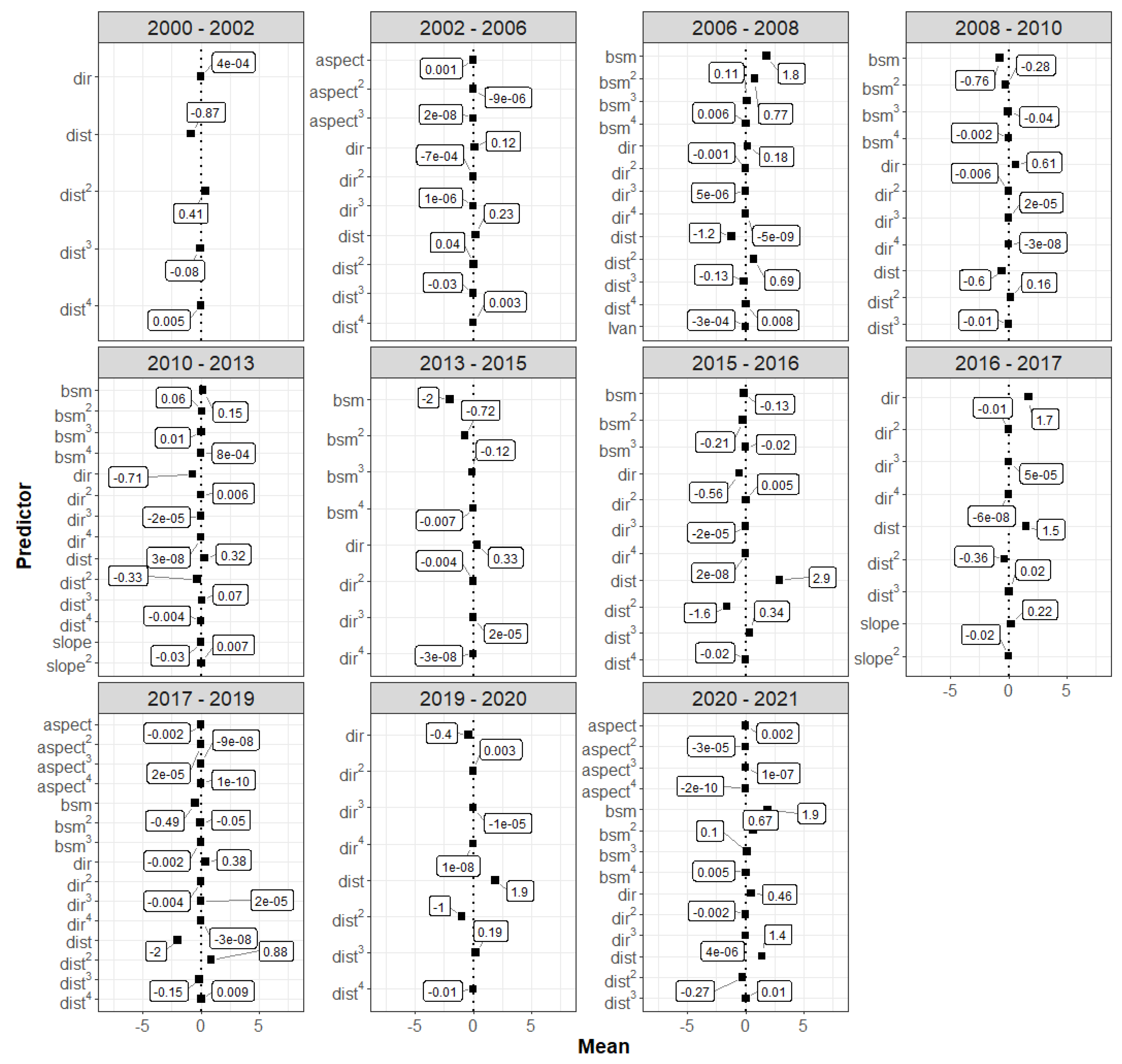
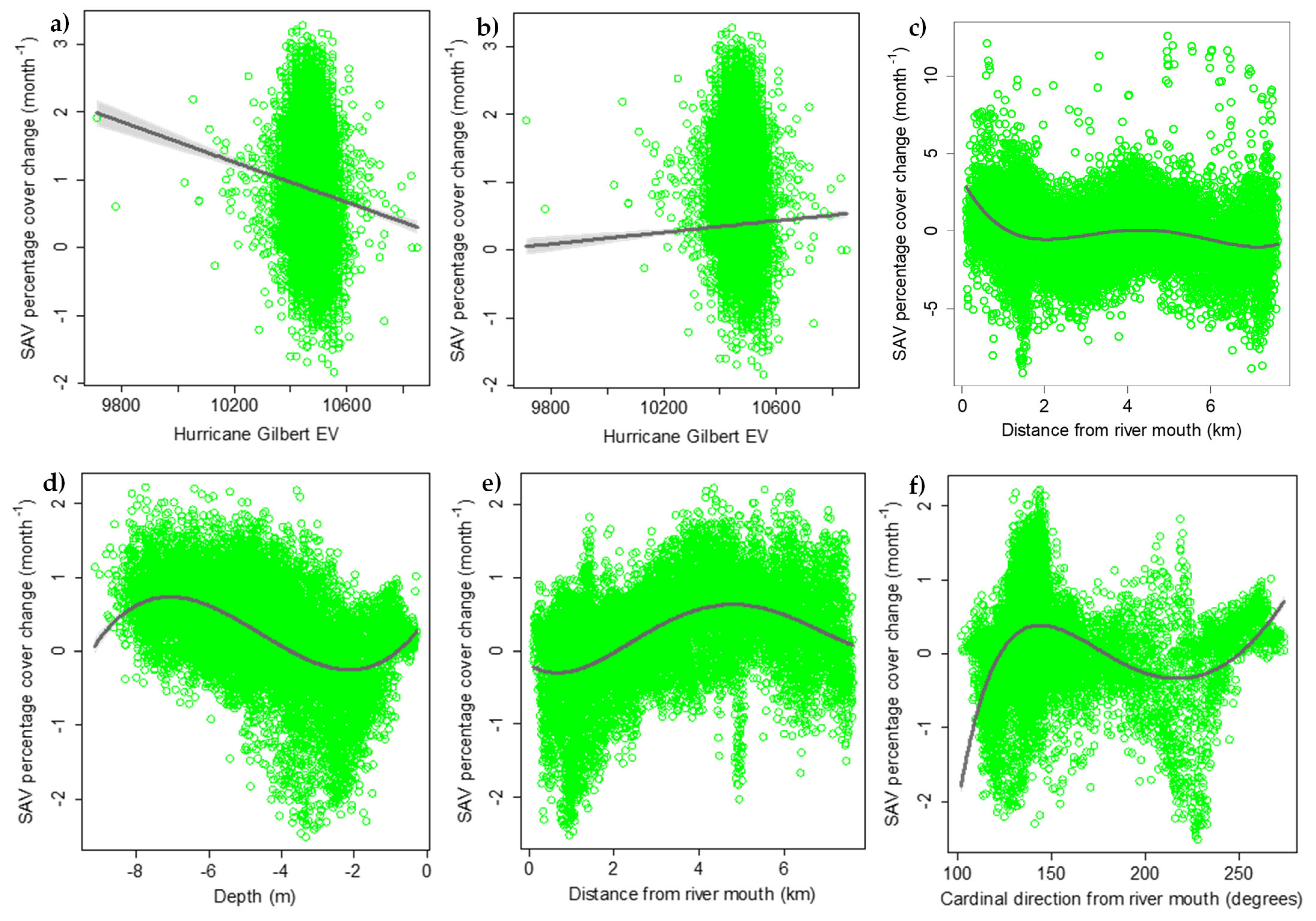
3.2. Spatial Pattern Predictors

The pixel-based regression was used to determine if rainfall influenced the spatial patterns of SAV loss, gain, and percentage area change. For loss and gain, this was found to be confined largely to a small area, which was close to the mouth of the main river towards the northwestern section of the bay (Figure 5). The influence of rainfall on both loss and gain was negative and positive, that is, SAV probability of loss or gain increased or decreased with an increase in monthly rainfall (Figure 6). There were more locations with a probability of SAV loss declining or the SAV gain increasing as rainfall increased than areas with the opposite trend (Figure 5). Rainfall influenced SAV percentage cover change over a larger area of the bay (when compared with SAV loss and gain), and these were interspersed with areas that were not affected (Figure 5). Also, rainfall had both a positive and negative effect on percentage cover change, with the predominant effect being positive (Figure 5 and Figure 6).

We identified the most important spatial pattern predictors of SAV cover loss, gain, and percentage cover change to determine other possible influences on change. All final models that included the most important predictors had an AUC of >0.6. Marginal R-squared values for important predictors of SAV loss ranged from 0.2 to 19.2%, with the highest value being obtained during the 2008–2010 period (Figure 7). The third (2002–2006) highest R-squared value (15.5%; Figure 7) was obtained during the period when SAV loss was highest after the passage of a single hurricane in 2004. A single predictor of SAV loss was found to be important during 13 of the 23 periods assessed, whereas multiple predictors were important for the remaining periods (Figure 8). Like the pixel-based regression results, the important predictors had a positive or a negative effect on SAV loss (Figure 8 and Figure 9a–c), and the relationship between SAV loss and the predictors were either linear (SAV loss increased or decreased with an increase in BSM, aspect, slope, distance, direction, or EV) or they were better explained by a polynomial regression (Figure 8 and Figure 9a–c), indicating that their effects varied across a range of predictor values. The most frequent important predictors of SAV loss were direction (eleven intervals) and distance (seven intervals) from the mouth of the river, followed by aspect, BSM, slope, and then average EV (six, six, two, and one intervals, respectively) (Figure 8). This highlighted the importance of rainfall (which influences river outflow), as the probability of SAV loss declined significantly as distance from the river mouth increased (Figure 9c); for six of seven intervals, it was important (the parameter estimates were (largely) negative (Figure 8)). Moreover, nearly all the relationships with direction from river (10 of 11), were positive, indicating that the highest probability of loss occurred largely to the southwest to northwest of the river mouth (Figure A3). Only during the 2002–2006 period was the probability of loss higher to the east of the river mouth as well as the southwest to the northwest (Figure 9b). Additionally, SAV loss was more likely to occur in shallow areas (four of the six intervals), that is, there was a positive relationship with BSM. BSM values are negative (Figure A3); therefore, a positive relationship indicates a greater probability of loss in shallow areas (Figure 8). The results also highlighted the possible impact of two hurricanes. Aspect was an important predictor of the probability of loss during the period when Ivan passed by the island (2002–2006). Aspect is used in the calculation of EV and is a proxy to the predominant direction of exposure to hurricane winds [36,52]. Our results show that SAV loss was greatest at benthic locations with a northwestern and a northern facing aspect (Figure 9g,h), and this corresponded with the prevailing wind direction of the leading edge of the outer wind bands of Ivan (Figure A4). Also, during this period, the probability of loss for the first time was higher to the east and southwest–northwest of the river mouth (therefore, loss occurred in more than one direction) (Figure 9b and Figure A3). Furthermore, average EV (for Ivan and Dean) was an important predictor during the 2010–2013 period, where SAV loss was positively associated with higher average EV (Figure 8 and Figure 9a).

Marginal R-squared values for the predictors of SAV cover gain ranged from 0.04 to 37.2%, with the highest value being obtained during the 2010–2013 period (Figure 7) when SAV cover was recovering following the passage of two hurricanes. A single predictor of SAV gain was found to be important during eight of the twenty-three periods assessed, whereas multiple predictors were important for the remaining periods (Figure 10). Additionally, there were no important predictors for SAV gain during one period (1986–1987). Also, the most important predictors had a positive or a negative effect on SAV gain, and the influences of the predictors were best explained by linear or polynomial relationships (Figure 9d–f and Figure 10). Like SAV loss, SAV gain was most frequently predicted by direction and distance (eleven and nine intervals, respectively), followed by BSM, aspect, slope, and Hurricane Ivan EV (eight, six, six, and one intervals, respectively) (Figure 10). These results again highlighted that proximity to the mouth of the river influenced dynamic changes. Specifically, SAV gain was positively related to the direction from the river mouth for nine of eleven periods when the latter was important, and like SAV loss, this indicated that the highest probability of gain occurred largely to the southwest to northwest of the river mouth. Also, SAV loss was higher closer to the river mouth during five of nine intervals. The probability of SAV gain was highest at shallow locations (six of eight periods; Figure 9f) than at greater depths (only two periods) (Figure 9). Moreover, there was greater SAV gain where Hurricane Ivan EV was highest during the period (2006–2008) (Figure 9d and Figure 10) that followed the passage of Ivan in 2004, indicating that SAV cover was recovering at sites that were impacted by Ivan but not by Dean.

Marginal R-squared values for the predictors of percentage cover change ranged from 8.3 to 54.7%, with the highest value being obtained during the 2015–2016 period (Figure 7). Also, multiple predictors were largely found to be important (Figure 11 and Figure 12). The most common relationship was polynomial, indicating that the influence of the predictors varied across the range of values for the predictors, and again the relationships can either be positive or negative (Figure 11, Figure 12 and Figure 13a–f). The most frequent important predictors were distance and direction from the river mouth (21 and 19 intervals, respectively). This was followed by BSM, slope, aspect, and EV (twelve, five, five, and three intervals, respectively). Unlike SAV loss and gain, percentage cover change may have been influenced by hurricanes three times (Figure 11, Figure 12 and Figure 13a,b). Hurricane Gilbert EV negatively influenced SAV percentage cover change during the period when Gilbert made landfall (1987–1988), but this changed to a positive relationship during the period after the hurricane (1988–1990), indicating the recovery of SAV cover in high-EV areas (Figure 11 and Figure 13a,b). Hurricane Ivan EV had a negative influence when other predictors influenced SAV percentage cover change during the period after the hurricane passed the island (2006–2008), which is possibly a lag effect (Figure 11).

4. Discussion

In this study, we identified various factors that influenced SAV extent and percentage cover over a period of 37 years. We used data and maps generated from a random forest regression model that used 2013 hydroacoustic data to predict SAV percentage cover from reflectance data from 24 Landsat satellite images that were collected during the period 1984–2021. Our assessments were based on several assumptions. We used level 2 processed images with atmospheric correction, which should standardize the reflectance data for each image. This is important, as we were not able to determine the accuracy of the SAV percentage cover maps generated for the years before or after 2013. Because the images were standardized, it is expected that the reflectance values would fall within a similar range, and therefore, the SAV percentage cover maps should have similar accuracies. We also made this assumption when using/applying thresholds for converting SAV percentage cover to binary, that is, the thresholds would produce maps with similar accuracies to our 2013 thematic maps. Nevertheless, we were able to use the resulting maps/data from the maps to identify how several factors influenced seagrass cover change at our study site.

4.1. Spatial Pattern Predictors of SAV Change

There have been reported declines in seagrass cover due to a variety factors including natural hazards such as single [18] or multiple storms/cyclones/hurricanes [17], droughts [21], a combination of droughts and storms/cyclones/hurricanes [21,67], a combination of storms and cyclones and above average rainfall [68], and due to anthropogenic activities, despite protection [23]. However, several studies have reported stable SAV cover [69] or an expansion/increase in SAV area due to increased protection [9] or despite the impacts of multiple storms [20]. We found that seagrass percentage cover and extent in the BBSFCA were largely stable over the 37-year period and SAV loss and gain for several periods were explained by proximity to the mouth of a river. The spatial pattern analysis using the pixel-based regression and the spatial Bayesian INLA models confirmed that an area of active/dynamic change can be found close to the mouth of the river, towards the western side of the bay. We found that annual rainfall was at historic lows and higher monthly rainfall had a positive influence on seagrass percentage cover. The pixel-based regression confirmed the latter, specifically that overall, higher rainfall largely had a positive influence on SAV gain and percentage cover change. This is contrary to the findings of several studies that have reported that higher rainfall results in increased surface runoffs or outflows from rivers into bays, and this is generally associated with increased turbidity and nutrients, which increases SAV stress and reduces extent or cover ([70]) and vertical growth [71]. Flood outflows can increase these impacts significantly (2–3-fold increases in turbidity and nutrients), resulting in an even greater decline in seagrasses [72]. Droughts can result in increased evaporation of water and salinity (creating hypersaline conditions) and bottom-water anoxia, leading to a reduction in SAV cover and extent [19], particularly during low tides in intertidal areas [73]. Also, seasonal rainfall is associated with lower and higher SAV percentage cover/extent during the wet and dry seasons, respectively [70,74]. Our result is therefore unusual, and even after reviewing studies of freshwater SAVs [75], higher rainfall has not been reported to be associated with an increase in SAV percentage cover and/or extent. Higher rainfall does result in increased turbidity in the BBSFCA, as we were not able to use images collected during several years because of high turbidity around the mouth of the river, or across most of the western half of the bay. Also, the predominant sediment type found in the persistently bare area to the west of the bay (and the mouth of the river) and close to the coastline is silt [30], indicating that there is a constant input of terrigenous sediment. However, we did not examine the effects of monthly rainfall using seagrass cover data collected every month [70]. Instead, we calculated monthly rates of percentage cover change, and recorded SAV loss and gain using images captured over a minimum period of 4 months to a maximum period of 46 months, due to the unavailability of suitable images. Also, rainfall in Jamaica and on the south coast is seasonal; therefore, we likely captured the overall response of SAVs to rainfall irrespective of season, that is, before, after, or during one or more wet and/or dry seasons. Nevertheless, seagrass meadows/beds have been found to be nutrient-limited [76,77], and therefore, moderate increases in nutrients are beneficial [78]; high inputs, however, are detrimental, as it promotes the growth and dominance of competing macroalgae [78,79]. Additionally, although there have been reported declines in seagrass percentage cover during wet seasons, this can be followed by rapid recovery during the following dry season [70]. Furthermore, nutrients that are brought by outflows or runoffs during the rainy season are thought to contribute to the recovery of seagrass percentage cover during the dry season that follows the rainy season [70]. This can perhaps be used to explain our results. That is, over time, SAV in the bay benefitted from higher overall inputs of nutrients from outflows during the rainy season. Moreover, the bay is currently receiving < 1000 mm of the total annual rainfall it received at the turn of the 20th century, yet SAV extent was largely maintained, and percentage cover in most of the bay was >80%, six out of the twenty-four times it was mapped, the most recent being in 2019. It is conceivable that the bay might be receiving less nutrients than it did over 100 years ago, especially during periods of low rainfall. However, there has been extensive agricultural (along the river course) and coastal developments, and perhaps this is compensating for a reduction in nutrient inputs. We are currently investigating whether the positive effect of rainfall is maintained when images with higher temporal and spatial resolutions are used.

There was a significant decline in SAV area/extent during one period, 2002–2006, when the island was impacted by Hurricane Ivan. The effects of Ivan may have been compounded by a second hurricane (Dean) three years later (Figure A4). As a result, SAV extent/area did not fully recover until the 2013–2015 period, or 9–11 years after the impact of the first hurricane. The identified important spatial pattern predictors can be used as evidence for the impact of Ivan and Dean; specifically, direction from the mouth of the river and aspect were the most important predictors of SAV loss during the 2002–2006 period. For the first of the two predictors, this was the first time that the probability of SAV loss was equally high on both sides of or multiple cardinal directions from the mouth of the river (southeast and southwest to the northwest; Figure 8 and Figure A3), indicating that there was a higher than usual outflow from the river. This may have influenced SAV loss, due to exceedingly high rainfall during hurricane events, which can be detrimental to seagrass beds [80]. The net effect was an increase in the extent of the SAV absent class around the mouth of the river, which for the first time extended from the southwest and west to the southeast of the river mouth (Figure 3). Also, percentage cover around the river fell to ≤20% for the first time (Figure 2). Following the hurricanes, direction or distance from the river mouth was an important predictor of SAV loss for every period until 2013–2015, during which the size of the SAV absent class close to the river increased (Figure 3 and Figure 8). SAV did not recolonize the newly transformed SAV absent areas until 2015 (Figure 3 and Figure 8). The second important predictor, aspect, was used in the calculation of EV, and it is a proxy to the predominant direction of exposure to hurricane winds [36,52]. It can also confound the influence of EV, as it can be a more important predictor of hurricane damage if the impact of a hurricane is strong in a given/particular direction, because the winds are moving predominantly in that direction [52]. Our results showed that SAV loss was greatest in areas on the benthos that had a northwestern to northern facing aspect (Figure 9g,h and Figure A3). This corresponded with the prevailing wind direction of the leading edge (the most destructive/strongest winds) of the outer wind bands of Ivan (Figure A4). Several studies that have employed the use of wave models have reported similar directional impacts of storms on seagrass beds/meadows; these impacts were also associated with the prevailing direction of the storm winds [81,82]. Also, seagrass declines following storms are usually associated with persistent changes in seawater quality and burial [83]. Greater exposure to the direction of the prevailing winds of a storm was one of two factors that explained the depth of burial of seagrasses found along the Spanish Mediterranean coast (higher exposure to storm winds increased burial depths) that were impacted by Storm Gloria in 2020 [82]. Burial may have been the main impact of Ivan, as there were several bare sand patches present during the 2006–2013 period (Figure 3), one of which was described as a “sand bar” by [30]. These bare patches were not present in the maps of benthic classes before 2006 or after 2013 (Figure 3). The “sand bar” first appeared in the south-eastern section of the bay in 2006, in an area previously covered by seagrass (Figure 3). By 2015, however, the “sand bar” and all the bare sand patches were recolonized and were no longer visible in the benthic feature maps (Figure 3).

We also found evidence of the cumulative impact of two hurricanes that follow similar tracks. The first evidence was that there was SAV gain/recovery and positive SAV percentage cover change at some sites on the benthos during 2006–2008 which were exposed to Hurricane Ivan in 2004, and this recovery/change preceded a complete recovery of all impacted areas/sites in 2015. These were likely to be sites/locations that were impacted by Ivan in 2004, but not by Dean in 2007, and were recovering during this period, while other areas impacted by both hurricanes continued to experience a loss up until 2013. Moreover, the cumulative effects of Ivan and Dean (average EV) explained (although the marginal R-squared was low) the pattern of SAV loss (higher average EV was associated with a higher probability of loss) during 2010–2013, 9 and 6 years after Ivan and Dean, respectively, which impacted our study site. This likely contributed to the (relatively) long period it took for SAV extent/area to recover (close to decade). The cumulative negative impacts of storms have been reported elsewhere. For example, on the southwestern coast of Korea, the cumulative effects of three consecutive typhoons in two months resulted in a seagrass meadow completely dying off, despite previous (single) typhoons having little or no impact [17]. The contrasting impacts of previous single typhoons versus the three consecutive typhoons also indicate that the damage caused by storms, hurricanes, cyclones, or typhoons can be very variable and range from no damage to complete degradation, die-off, or habitat destruction [20,83]. We also found that the impacts of different hurricanes on SAV in the BBSFCA can vary. While Ivan and Dean impacted SAV extent, Hurricane Gilbert did not have a similar impact, but instead may have reduced seagrass percentage cover during the period 1987–1988, and it recovered immediately during the period that followed (1988–1990). Similarly, the short-term impacts of a cyclone on seagrasses in southwestern Madagascar included a decline in percentage cover and height [18]. Our observed differences in impact may be explained by the tracks of the hurricanes (and distance of the eye from the island). The strongest winds or leading edge of hurricanes with a track close to the south of Jamaica will cover most of the island, tend to have a predominantly northern wind direction, and will have a greater impact on the south coast (Figure A4). Hurricane Gilbert made landfall and as such, the proxy hurricane indicated that the leading edge of the hurricane would have been largely offshore to the north of the island, with only the trailing weaker wind bands affecting the BBSFCA on the south coast (Figure A4). These patterns of impact mirror the impacts of hurricanes on forest ecosystems in Jamaica, where the track and distance of the eye of a hurricane from the island (and whether they pass to the south, north, or make landfall) can be used to determine the sites/locations that experienced the greatest impacts [36].

Depth and benthic topography have been previously reported as being important predictors of seagrass presence, density, or percentage cover, but there is a paucity of studies on how they influence dynamic changes. Seagrasses were found to colonize a gentle slope with an inclination of 0.0 to 56.6 degrees along the coast of Giglio Island, Italy [24]. Also, seagrass cover increased with higher slope values and depth in shallow areas [24]. Shoot density decreased non-linearly with depth, with peak densities being found at intermediate depths in a fringing-reef lagoon in the Mexican Caribbean [84]. Additionally, seagrass distribution in shallow water can be limited by exposure to wind and wave, or where exposure to waves is greater, whereas in deeper water, they are limited by light [84,85]. As stated previously, aspect can give an indication of directional impact or areas predominantly exposed to a specific wave/wind direction. For the BBSFA, the average slope percentage, aspect, and depth were 0.8% (or equivalent to 0.4 degrees), 206 degrees, or a predominant southwestern facing aspect, and 4.2 m (range: 0.05–9.3 m), respectively. SAV was present across the entire bay over our study period and therefore was not limited by depth or benthic topography. However, we found that the probability of SAV loss and gain was higher in shallow areas, mainly around the mouth of the river, indicating that these were areas of dynamic change in the BBSFCA. High sediment input and greater exposure to wave action and wind may have influenced dynamic changes in these areas. Some shallow areas, however, may have been impacted by anthropogenic activities, as there was a large beach and other smaller public beaches and several beaches associated with lower-impact coastal developments (small higher-end resorts) found in shallow areas along the coast. Slope and aspect were the least selected benthic topographic predictors of spatial pattern change. Topographic variation was subtle in this bay, and this perhaps can explain the low importance of slope and aspect. Nevertheless, aspect was an important indicator of/proxy to Hurricane Ivan impact.

4.2. Implications for Management

SAV cover was stable before and continued to be stable after the BBSFCA was established. Consequently, the BBSFCA is working, that is, it is helping to maintain SAV cover. The main area of dynamic change was around the mouth of the main river that drains into the bay, with one area towards the west end of the bay being consistently bare. Under normal circumstances, we would recommend that the BBSFCA managers integrate land–sea or ridge-to-reef conservation planning [10,11,12] to address the threat posed by high terrigenous sediment load in river outflows. But this might be beyond the of the remit of the present managers. Additionally, rainfall, and hence river outflow, may be important due to its positive impact on SAV loss, gain, and percentage cover change, and given the significant reduction in annual rainfall. Moreover, hurricanes pose the greatest threat to the maintenance of SAV cover. We showed that the cumulative impacts of two hurricanes that followed a similar track to the south of the island can reduce SAV extent for an extended period. Even a single hurricane that made landfall and had less of an impact (Hurricane Gilbert) can reduce percentage cover. The island was impacted by four hurricanes in 8 years (Hurricanes Ivan (2004), Dennis (2005), Dean (2007), and Sandy (2012)), but only two of the four hurricanes passed to the north of the island. In the future, successive hurricanes that pass to the south of the island will have the capacity to substantially reduce SAV cover. Depth was found to be an important predictor of SAV dynamic change, and although this was primarily limited to shallow areas around the river mouth, loss may also be occurring in shallow areas with high anthropogenic activity (beaches and coastal developments). This, however, will need to be verified, and there is also a need to further verify the positive effect of rainfall using data with higher temporal and spatial resolutions. If the latter is found to be important, a further reduction in rainfall will also have serious implications for management.

5. Conclusions

We were able to document changes in SAV extent and percentage cover in the BBSFCA over a period of 37 years using data from 24 percentage cover and benthic features maps. These maps were generated by first building a random forest regression model with 2013 percentage cover hydroacoustic data (dependent variable) and reflectance data from 2013 Landsat 7 and 8 satellite images and auxiliary data as the predictors and then using the model to predict percentage cover using data from the Landsat satellite series. A threshold was applied to the percentage cover maps to generate the benthic features maps. We demonstrated that SAV cover was quite stable and possibly quite healthy, with several years with >80% percentage cover over most of the bay. There was a significant loss in SAV area between 2006 and 2013, with a subsequent recovery in 2015. We found that this loss may have initially occurred due to the impact of Hurricane Ivan in 2004, and this was compounded by a second hurricane (Dean) in 2007, which may have delayed the recovery of SAV extent until a decade after Ivan. Rainfall, and by extension outflow from the main river that drains into the bay, had an overall positive effect and is contributing significantly to SAV loss, gain, and percentage cover change, despite annual rainfall being approximately 1000 mm less on average than it was at the turn of the 20th century. We surmised that a loss of nutrient input caused by reduced outflows may have been supplemented by increased nutrient loads from agricultural and coastal developments. Shallow areas around the river mouth, and possibly areas close to coastal developments and beaches, were also active areas of change. An increase in the frequency of high-intensity hurricanes and an increase in the variability of rainfall in Jamaica, which can perhaps explain a reduction in annual rainfall at the BBSFA, will impact the site in the future.

References

1. Orth, R.J.; Carruthers, T.J.; Dennison, W.C.; Duarte, C.M.; Fourqurean, J.W.; Heck, K.L.; Hughes, A.R.; Kendrick, G.A.; Kenworthy, W.J.; Olyarnik, S. A global crisis for seagrass ecosystems. Bioscience 2006, 56, 987–996. [Google Scholar] [CrossRef]
2. Unsworth, R.K.; McKenzie, L.J.; Collier, C.J.; Cullen-Unsworth, L.C.; Duarte, C.M.; Eklöf, J.S.; Jarvis, J.C.; Jones, B.L.; Nordlund, L.M. Global challenges for seagrass conservation. Ambio 2019, 48, 801–815. [Google Scholar] [CrossRef] [PubMed]
3. Ralph, P.; Durako, M.J.; Enriquez, S.; Collier, C.; Doblin, M. Impact of light limitation on seagrasses. J. Exp. Mar. Biol. Ecol. 2007, 350, 176–193. [Google Scholar] [CrossRef]
4. Horinouchi, M. Distribution patterns of benthic juvenile gobies in and around seagrass habitats: Effectiveness of seagrass shelter against predators. Estuar. Coast. Shelf Sci. 2007, 72, 657–664. [Google Scholar] [CrossRef]
5. Unsworth, R.K.; Nordlund, L.M.; Cullen-Unsworth, L.C. Seagrass meadows support global fisheries production. Conserv. Lett. 2019, 12, e12566. [Google Scholar] [CrossRef]
6. Edgar, G.J.; Shaw, C. The production and trophic ecology of shallow-water fish assemblages in southern Australia I. Species richness, size-structure and production of fishes in Western Port, Victoria. J. Exp. Mar. Biol. Ecol. 1995, 194, 53–81. [Google Scholar] [CrossRef]
7. Grech, A.; Chartrand-Miller, K.; Erftemeijer, P.; Fonseca, M.; McKenzie, L.; Rasheed, M.; Taylor, H.; Coles, R. A comparison of threats, vulnerabilities and management approaches in global seagrass bioregions. Environ. Res. Lett. 2012, 7, 024006. [Google Scholar] [CrossRef]
8. Waycott, M.; Duarte, C.M.; Carruthers, T.J.; Orth, R.J.; Dennison, W.C.; Olyarnik, S.; Calladine, A.; Fourqurean, J.W.; Heck Jr, K.L.; Hughes, A.R. Accelerating loss of seagrasses across the globe threatens coastal ecosystems. Proc. Natl. Acad. Sci. USA 2009, 106, 12377–12381. [Google Scholar] [CrossRef]
9. Lefcheck, J.S.; Orth, R.J.; Dennison, W.C.; Wilcox, D.J.; Murphy, R.R.; Keisman, J.; Gurbisz, C.; Hannam, M.; Landry, J.B.; Moore, K.A. Long-term nutrient reductions lead to the unprecedented recovery of a temperate coastal region. Proc. Natl. Acad. Sci. USA 2018, 115, 3658–3662. [Google Scholar] [CrossRef] [PubMed]
10. Nordlund, L.M.; de la Torre-Castro, M.; Erlandsson, J.; Conand, C.; Muthiga, N.; Jiddawi, N.; Gullström, M. Intertidal zone management in the Western Indian Ocean: Assessing current status and future possibilities using expert opinions. Ambio 2014, 43, 1006–1019. [Google Scholar] [CrossRef] [PubMed]
11. Carlson, R.R.; Foo, S.A.; Asner, G.P. Land use impacts on coral reef health: A ridge-to-reef perspective. Front. Mar. Sci. 2019, 6, 562. [Google Scholar] [CrossRef]
12. Fache, E.; Pauwels, S. The ridge-to-reef approach on Cicia Island, Fiji. Ambio 2022, 51, 2376–2388. [Google Scholar] [CrossRef]
13. Brierley, A.S.; Kingsford, M.J. Impacts of climate change on marine organisms and ecosystems. Curr. Biol. 2009, 19, R602–R614. [Google Scholar] [CrossRef] [PubMed]
14. Knutson, T.R.; McBride, J.L.; Chan, J.; Emanuel, K.; Holland, G.; Landsea, C.; Held, I.; Kossin, J.P.; Srivastava, A.; Sugi, M. Tropical cyclones and climate change. Nat. Geosci. 2010, 3, 157–163. [Google Scholar] [CrossRef]
15. Chiang, F.; Mazdiyasni, O.; AghaKouchak, A. Evidence of anthropogenic impacts on global drought frequency, duration, and intensity. Nat. Commun. 2021, 12, 2754. [Google Scholar] [CrossRef] [PubMed]
16. Thornton, P.K.; Ericksen, P.J.; Herrero, M.; Challinor, A.J. Climate variability and vulnerability to climate change: A review. Glob. Chang. Biol. 2014, 20, 3313–3328. [Google Scholar] [CrossRef] [PubMed]
17. Kim, K.; Choi, J.-K.; Ryu, J.-H.; Jeong, H.J.; Lee, K.; Park, M.G.; Kim, K.Y. Observation of typhoon-induced seagrass die-off using remote sensing. Estuar. Coast. Shelf Sci. 2015, 154, 111–121. [Google Scholar] [CrossRef]
18. Côté-Laurin, M.-C.; Benbow, S.; Erzini, K. The short-term impacts of a cyclone on seagrass communities in Southwest Madagascar. Cont. Shelf Res. 2017, 138, 132–141. [Google Scholar] [CrossRef]
19. Hall, M.O.; Furman, B.T.; Merello, M.; Durako, M.J. Recurrence of Thalassia testudinum seagrass die-off in Florida Bay, USA: Initial observations. Mar. Ecol. Prog. Ser. 2016, 560, 243–249. [Google Scholar] [CrossRef]
20. León-Pérez, M.C.; Armstrong, R.A.; Hernández, W.J.; Aguilar-Perera, A.; Thompson-Grim, J. Seagrass cover expansion off Caja de Muertos Island, Puerto Rico, as determined by long-term analysis of historical aerial and satellite images (1950–2014). Ecol. Indic. 2020, 117, 106561. [Google Scholar] [CrossRef]
21. Congdon, V.M.; Hall, M.O.; Furman, B.T.; Campbell, J.E.; Durako, M.J.; Goodin, K.L.; Dunton, K.H. Common ecological indicators identify changes in seagrass condition following disturbances in the Gulf of Mexico. Ecol. Indic. 2023, 156, 111090. [Google Scholar] [CrossRef]
22. Chollett, I.; Bone, D.; Pérez, D. Effects of heavy rainfall on Thalassia testudinum beds. Aquat. Bot. 2007, 87, 189–195. [Google Scholar] [CrossRef]
23. Evans, S.M.; Griffin, K.J.; Blick, R.A.; Poore, A.G.; Vergés, A. Seagrass on the brink: Decline of threatened seagrass Posidonia australis continues following protection. PLoS ONE 2018, 13, e0190370. [Google Scholar] [CrossRef] [PubMed]
24. Mancini, G.; Mastrantonio, G.; Pollice, A.; Lasinio, G.J.; Belluscio, A.; Casoli, E.; Pace, D.S.; Ardizzone, G.; Ventura, D. Detecting trends in seagrass cover through aerial imagery interpretation: Historical dynamics of a Posidonia oceanica meadow subjected to anthropogenic disturbance. Ecol. Indic. 2023, 150, 110209. [Google Scholar] [CrossRef]
25. Lecours, V. On the use of maps and models in conservation and resource management (warning: Results may vary). Front. Mar. Sci. 2017, 4, 288. [Google Scholar] [CrossRef]
26. Barrell, J.; Grant, J. Detecting hot and cold spots in a seagrass landscape using local indicators of spatial association. Landsc. Ecol. 2013, 28, 2005–2018. [Google Scholar] [CrossRef]
27. Phinn, S.; Roelfsema, C.; Dekker, A.; Brando, V.; Anstee, J. Mapping seagrass species, cover and biomass in shallow waters: An assessment of satellite multi-spectral and airborne hyper-spectral imaging systems in Moreton Bay (Australia). Remote Sens. Environ. 2008, 112, 3413–3425. [Google Scholar] [CrossRef]
28. Baumstark, R.; Dixon, B.; Carlson, P.; Palandro, D.; Kolasa, K. Alternative spatially enhanced integrative techniques for mapping seagrass in Florida’s marine ecosystem. Int. J. Remote Sens. 2013, 34, 1248–1264. [Google Scholar] [CrossRef]
29. Vahtmäe, E.; Paavel, B.; Kutser, T. How much benthic information can be retrieved with hyperspectral sensor from the optically complex coastal waters? J. Appl. Remote Sens. 2020, 14, 016504. [Google Scholar] [CrossRef]
30. McIntyre, K.; McLaren, K.; Prospere, K. Mapping shallow nearshore benthic features in a Caribbean marine-protected area: Assessing the efficacy of using different data types (hydroacoustic versus satellite images) and classification techniques. Int. J. Remote Sens. 2018, 39, 1117–1150. [Google Scholar] [CrossRef]
31. McLaren, K.; McIntyre, K.; Prospere, K. Using the random forest algorithm to integrate hydroacoustic data with satellite images to improve the mapping of shallow nearshore benthic features in a marine protected area in Jamaica. GISci. Remote Sens. 2019, 56, 1065–1092. [Google Scholar] [CrossRef]
32. Newman, M.E.; McLaren, K.P.; Wilson, B.S. Long-term socio-economic and spatial pattern drivers of land cover change in a Caribbean tropical moist forest, the Cockpit Country, Jamaica. Agric. Ecosyst. Environ. 2014, 186, 185–200. [Google Scholar] [CrossRef]
33. Lambin, E.F.; Geist, H.J.; Lepers, E. Dynamics of land-use and land-cover change in tropical regions. Annu. Rev. Environ. Resour. 2003, 28, 205–241. [Google Scholar] [CrossRef]
34. Kamwi, J.M.; Cho, M.A.; Kaetsch, C.; Manda, S.O.; Graz, F.P.; Chirwa, P.W. Assessing the spatial drivers of land use and land cover change in the protected and communal areas of the Zambezi Region, Namibia. Land 2018, 7, 131. [Google Scholar] [CrossRef]
35. McIntyre, K. Benthic Mapping of the Bluefields Bay Fish Sanctuary, Jamaica. Master’s Thesis, Lund University, Lund, Sweden, 2015. [Google Scholar]
36. McLaren, K.; Luke, D.; Tanner, E.; Bellingham, P.J.; Healey, J.R. Reconstructing the effects of hurricanes over 155 years on the structure and diversity of trees in two tropical montane rainforests in Jamaica. Agric. For. Meteorol. 2019, 276, 107621. [Google Scholar] [CrossRef]
37. Majka, D.; Jenness, J.; Beier, P. CorridorDesigner: ArcGIS Tools for Designing and Evaluating Corridors. Available online: http://corridordesign.org (accessed on 15 February 2024).
38. R Core Team, R. R: A Language and Environment for Statistical Computing. R Foundation for Statistical Computing-4.3.1. Available online: http://www.R-project.org (accessed on 25 October 2023).
39. R Core Team, R. R: A Language and Environment for Statistical Computing. R Foundation for Statistical Computing-glcm” Package. Available online: http://www.R-project.org (accessed on 25 October 2023).
40. Zvoleff, A. Package ‘glcm’. Calculate Textures from Grey-Level Co-Occurence Matrices (GLCMs). Available online: https://cran.r-project.org/web/packages/glcm/index.html (accessed on 25 October 2022).
41. Liaw, A.; Wiener, M. Classification and regression by randomForest. R News 2002, 2, 18–22. [Google Scholar]
42. Bakar, K.S.; Sahu, S.K. spTimer: Spatio-temporal Bayesian modeling using R. J. Stat. Softw. 2015, 63, 1–32. [Google Scholar] [CrossRef]
43. Aho, K. Asbio: A Collection of Statistical Tools for Biologists_. R package Version 1.9-6. Available online: https://CRAN.R-project.org/package=asbio (accessed on 15 February 2022).
44. Wood, S.N. Fast stable restricted maximum likelihood and marginal likelihood estimation of semiparametric generalized linear models. J. R. Stat. Soc. Ser. B Stat. Methodol. 2011, 73, 3–36. [Google Scholar] [CrossRef]
45. Wood, S.N. Generalized Additive Models: An Introduction with R; CRC Press: Boca Raton, FL, USA, 2017. [Google Scholar]
46. Wood, S.N. Stable and efficient multiple smoothing parameter estimation for generalized additive models. J. Am. Stat. Assoc. 2004, 99, 673–686. [Google Scholar] [CrossRef]
47. Wood, S.N.; Pya, N.; Säfken, B. Smoothing parameter and model selection for general smooth models. J. Am. Stat. Assoc. 2016, 111, 1548–1563. [Google Scholar] [CrossRef]
48. Zuur, A.F.; Ieno, E.N.; Walker, N.J.; Saveliev, A.A.; Smith, G.M. Mixed Effects Models and Extensions in Ecology with R; Springer: Berlin/Heidelberg, Germany, 2009; Volume 574. [Google Scholar]
49. Hyndman, R.; Athanasopoulos, G.; Bergmeir, C.; Caceres, G.; Chhay, L.; O’Hara-Wild, M.; Petropoulos, F.; Razbash, S.; Wang, E.; Yasmeen, F. Forecast: Forecasting Functions for Time Series and Linear Models. R package Version 8.21.1. Available online: https://pkg.robjhyndman.com/forecast/ (accessed on 15 February 2023).
50. Hyndman, R.J.; Khandakar, Y. Automatic time series forecasting: The forecast package for R. J. Stat. Softw. 2008, 27, 1–22. [Google Scholar] [CrossRef]
51. Bates, D.; Mächler, M.; Bolker, B.; Walker, S. Fitting linear mixed-effects models using lme4. arXiv 2014, arXiv:1406.5823. [Google Scholar]
52. Luke, D.; McLaren, K.; Wilson, B. Modeling hurricane exposure in a Caribbean lower montane tropical wet forest: The effects of frequent, intermediate disturbances and topography on forest structural dynamics and composition. Ecosystems 2016, 19, 1178–1195. [Google Scholar]
53. Lindgren, F.; Rue, H. Bayesian spatial modelling with R-INLA. J. Stat. Softw. 2015, 63, 25. [Google Scholar] [CrossRef]
54. Lindgren, F.; Rue, H.; Lindström, J. An explicit link between Gaussian fields and Gaussian Markov random fields: The stochastic partial differential equation approach. J. R. Stat. Soc. Ser. B Stat. Methodol. 2011, 73, 423–498. [Google Scholar] [CrossRef]
55. Rue, H.; Martino, S.; Chopin, N. Approximate Bayesian inference for latent Gaussian models by using integrated nested Laplace approximations. J. R. Stat. Soc. Ser. B Stat. Methodol. 2009, 71, 319–392. [Google Scholar] [CrossRef]
56. Rue, H.; Riebler, A.; Sørbye, S.H.; Illian, J.B.; Simpson, D.P.; Lindgren, F.K. Bayesian computing with INLA: A review. Annu. Rev. Stat. Its Appl. 2017, 4, 395–421. [Google Scholar] [CrossRef]
57. Martins, T.G.; Simpson, D.; Lindgren, F.; Rue, H. Bayesian computing with INLA: New features. Comput. Stat. Data Anal. 2013, 67, 68–83. [Google Scholar] [CrossRef]
58. Rue, H.; Martino, S. Approximate Bayesian inference for hierarchical Gaussian Markov random field models. J. Stat. Plan. Inference 2007, 137, 3177–3192. [Google Scholar] [CrossRef]
59. Cosandey-Godin, A.; Krainski, E.T.; Worm, B.; Flemming, J.M. Applying Bayesian spatiotemporal models to fisheries bycatch in the Canadian Arctic. Can. J. Fish. Aquat. Sci. 2015, 72, 186–197. [Google Scholar] [CrossRef]
60. Fuglstad, G.-A.; Simpson, D.; Lindgren, F.; Rue, H. Constructing priors that penalize the complexity of Gaussian random fields. J. Am. Stat. Assoc. 2019, 114, 445–452. [Google Scholar] [CrossRef]
61. Illian, J.B.; Sørbye, S.H.; Rue, H.; Hendrichsen, D.K. Using INLA to fit a complex point process model with temporally varying effects-a case study. J. Environ. Stat. 2012, 3, 1–25. [Google Scholar]
62. Spiegelhalter, D.J.; Best, N.G.; Carlin, B.P.; Van Der Linde, A. Bayesian measures of model complexity and fit. J. R. Stat. Soc. Ser. B Stat. Methodol. 2002, 64, 583–639. [Google Scholar] [CrossRef]
63. Zheng, B. Summarizing the goodness of fit of generalized linear models for longitudinal data. Stat. Med. 2000, 19, 1265–1275. [Google Scholar] [CrossRef]
64. Robin, X.; Turck, N.; Hainard, A.; Tiberti, N.; Lisacek, F.; Sanchez, J.-C.; Müller, M. pROC: An open-source package for R and S+ to analyze and compare ROC curves. BMC Bioinform. 2011, 12, 77. [Google Scholar] [CrossRef] [PubMed]
65. Sørbye, S.H. Tutorial: Scaling IGMRF-Models in R-INLA; University of Tromsø, Department of Mathematics and Statistics: Tromsø, Norway, 2013. [Google Scholar]
66. Rodemann, J.R.; James, W.R.; Santos, R.O.; Furman, B.T.; Fratto, Z.W.; Bautista, V.; Lara Hernandez, J.; Viadero, N.M.; Linenfelser, J.O.; Lacy, L.A. Impact of extreme disturbances on suspended sediment in western Florida Bay: Implications for seagrass resilience. Front. Mar. Sci. 2021, 8, 633240. [Google Scholar] [CrossRef]
67. McKenna, S.; Jarvis, J.; Sankey, T.; Reason, C.; Coles, R.; Rasheed, M. Declines of seagrasses in a tropical harbour, North Queensland, Australia, are not the result of a single event. J. Biosci. 2015, 40, 389–398. [Google Scholar] [CrossRef] [PubMed]
68. Shelton, A.O.; Francis, T.B.; Feist, B.E.; Williams, G.D.; Lindquist, A.; Levin, P.S. Forty years of seagrass population stability and resilience in an urbanizing estuary. J. Ecol. 2017, 105, 458–470. [Google Scholar] [CrossRef]
69. Ahmad-Kamil, E.; Ramli, R.; Jaaman, S.; Bali, J.; Al-Obaidi, J. The effects of water parameters on monthly seagrass percentage cover in Lawas, East Malaysia. Sci. World J. 2013, 2013, 892746. [Google Scholar] [CrossRef] [PubMed]
70. Marbà, N.; Duarte, C.M. Interannual changes in seagrass (Posidonia oceanica) growth and environmental change in the Spanish Mediterranean littoral zone. Limnol. Oceanogr. 1997, 42, 800–810. [Google Scholar] [CrossRef]
71. Campbell, S.J.; McKenzie, L.J. Flood related loss and recovery of intertidal seagrass meadows in southern Queensland, Australia. Estuar. Coast. Shelf Sci. 2004, 60, 477–490. [Google Scholar] [CrossRef]
72. de Fouw, J.; Govers, L.L.; van de Koppel, J.; van Belzen, J.; Dorigo, W.; Cheikh, M.A.S.; Christianen, M.J.; van der Reijden, K.J.; van der Geest, M.; Piersma, T. Drought, mutualism breakdown, and landscape-scale degradation of seagrass beds. Curr. Biol. 2016, 26, 1051–1056. [Google Scholar] [CrossRef] [PubMed]
73. Khogkhao, C.; Hayashizaki, K.-I.; Tuntiprapas, P.; Prathep, A. Changes in seagrass communities along the runoff gradient of the Trang river, Thailand. Sci. Asia 2017, 43, 339–346. [Google Scholar] [CrossRef]
74. Shivers, S.D.; Golladay, S.W.; Waters, M.N.; Wilde, S.B.; Ashford, P.D.; Covich, A.P. Changes in submerged aquatic vegetation (SAV) coverage caused by extended drought and flood pulses. Lake Reserv. Manag. 2018, 34, 199–210. [Google Scholar] [CrossRef]
75. Agawin, N.S.; Duarte, C.M.; Fortes, M.D. Nutrient limitation of Philippine seagrasses (Cape Bolinao, NW Philippines): In situ experimental evidence. Mar. Ecol. Prog. Ser. 1996, 138, 233–243. [Google Scholar] [CrossRef]
76. Terrados, J.; Agawin, N.S.; Duarte, C.M.; Fortes, M.D.; Kamp-Nielsen, L.; Borum, J. Nutrient limitation of the tropical seagrass Enhalus acoroides (L.) Royle in Cape Bolinao, NW Philippines. Aquat. Bot. 1999, 65, 123–139. [Google Scholar] [CrossRef]
77. Vieira, V.M.; Lobo-Arteaga, J.; Santos, R.; Leitão-Silva, D.; Veronez, A.; Neves, J.M.; Nogueira, M.; Creed, J.C.; Bertelli, C.M.; Samper-Villarreal, J. Seagrasses benefit from mild anthropogenic nutrient additions. Front. Mar. Sci. 2022, 9, 960249. [Google Scholar] [CrossRef]
78. Camacho, R.; Houk, P. Decoupling seasonal and temporal dynamics of macroalgal canopy cover in seagrass beds. J. Exp. Mar. Biol. Ecol. 2020, 525, 151310. [Google Scholar] [CrossRef]
79. Hernández-Delgado, E.A.; Toledo-Hernández, C.; Ruíz-Díaz, C.; Gómez-Andújar, N.; Medina-Muñiz, J.; Canals-Silander, M.; Suleimán-Ramos, S. Hurricane impacts and the resilience of the invasive sea vine, Halophila stipulacea: A case study from Puerto Rico. Estuaries Coasts 2020, 43, 1263–1283. [Google Scholar] [CrossRef]
80. Oprandi, A.; Mucerino, L.; De Leo, F.; Bianchi, C.; Morri, C.; Azzola, A.; Benelli, F.; Besio, G.; Ferrari, M.; Montefalcone, M. Effects of a severe storm on seagrass meadows. Sci. Total Environ. 2020, 748, 141373. [Google Scholar] [CrossRef] [PubMed]
81. Marco-Méndez, C.; Marbà, N.; Amores, Á.; Romero, J.; Minguito-Frutos, M.; García, M.; Pagès, J.F.; Prado, P.; Boada, J.; Sánchez-Lizaso, J.L. Evaluating the extent and impact of the extreme Storm Gloria on Posidonia oceanica seagrass meadows. Sci. Total Environ. 2024, 908, 168404. [Google Scholar] [CrossRef] [PubMed]
82. Correia, K.M.; Smee, D.L. A meta-analysis of tropical cyclone effects on seagrass meadows. Wetlands 2022, 42, 108. [Google Scholar] [CrossRef]
83. Enríquez, S.; Olivé, I.; Cayabyab, N.; Hedley, J.D. Structural complexity governs seagrass acclimatization to depth with relevant consequences for meadow production, macrophyte diversity and habitat carbon storage capacity. Sci. Rep. 2019, 9, 14657. [Google Scholar] [CrossRef] [PubMed]
84. Krause-Jensen, D.; Quaresma, A.L.; Cunha, A.H.; Greve, T. How are seagrass distribution and abundance monitored. Eur. Seagrasses Introd. Monit. Manag. 2004, 45–53. [Google Scholar]
85. Knapp, K.R.; Kruk, M.C.; Levinson, D.H.; Diamond, H.J.; Neumann, C.J. The international best track archive for climate stewardship (IBTrACS) unifying tropical cyclone data. Bull. Am. Meteorol. Soc. 2010, 91, 363–376. [Google Scholar] [CrossRef]
86. Knapp, K.R.; Diamond, H.J.; Kossin, J.P.; Kruk, M.C.; Schreck, C.J. International Best Track Archive for Climate Stewardship (IBTrACS) Project, Version 4. North Atlantic. NOAA Natl. Cent. Environ. Inf. 2018, 10. [Google Scholar] [CrossRef]
87. Mikita, T.; Klimánek, M. Topographic exposure and its practical applications. J. Landsc. Ecol. 2010, 3, 42–51. [Google Scholar] [CrossRef]
88. Batke, S.P.; Jocque, M.; Kelly, D.L. Modelling hurricane exposure and wind speed on a mesoclimate scale: A case study from Cusuco NP, Honduras. PLoS ONE 2014, 9, e91306. [Google Scholar] [CrossRef] [PubMed]
Figure 1. Maps showing (a) the Caribbean region, (b) the location of the Bluefields Bay Special Fish Conservation Area (BBSFCA) on the southwestern coast of Jamaica, (c) location of reference samples used for accuracy assessments, and (d) the hydroacoustic survey tracks. Blue box indicates the location of Jamaica and the study site.
Remotesensing 16 01247 g001
Figure 2. Maps of submerged aquatic vegetation percentage cover in the Bluefields Bay Special Fish Conservation Area (BBSFCA), Westmoreland, Jamaica that were produced/predicted by Landsat 7 and 8 random forest regression models for the period 1984–2021.
Remotesensing 16 01247 g002
Figure 3. Maps of benthic features in the Bluefields Bay Special Fish Conservation Area (BBSFCA), Westmoreland, Jamaica for the period 1984–2021 that were produced by applying a threshold to submerged aquatic vegetation (SAV) percentage cover maps generated from the SAV random forest regressions.
Remotesensing 16 01247 g003
Figure 4. Observed and predicted values obtained from our analyses using (a) a generalized additive mixed model (GAMM) with an autoregressive moving average (ARMA) error structure to assess change in total area of SAV over time in the Bluefields Bay Special Fish Conservation Area (BBSFCA), Westmoreland, Jamaica, (b) a generalized linear regression (GLM) with a gaussian link function used to determine the influence of monthly rainfall on SAV percentage cover change in the BBSFCA, and (c) a generalized additive model (GAM) used to assess the changes in total annual rainfall from 1901 to 2021 over time for Savanna-la-mar, the capital of Westmoreland, and the BBSFCA. Grey shadow/shade = standard error.
Remotesensing 16 01247 g004
Figure 5. Results obtained from the pixel-based regression used to assess the influence of monthly rainfall on the spatial pattern of (ac) SAV loss, (df) gain, and (gi) percentage cover change in the Bluefields Bay Special Fish Conservation Area (BBSFCA), Westmoreland, Jamaica. The outputs from the regressions are presented as maps and include the p-value (top row), the sign (+ or −) of the regression slope (middle row), and the R2 values.
Remotesensing 16 01247 g005
Figure 6. Examples of observed and predicted values for negative (in left column) and positive (in the right column) relationships identified by the pixel-based regressions that were used to assess the influence of monthly rainfall on the spatial pattern of SAV loss (top row), gain (middle row), and percentage cover change (bottom row) in the Bluefields Bay Special Fish Conservation Area (BBSFCA), Westmoreland, Jamaica. Grey shadow/shade = standard error. Black arrows = pixel location for the graphs.
Remotesensing 16 01247 g006
Figure 7. Marginal R-squared values calculated for the final parsimonious Bayesian Integrated Nested Laplace Approximation (INLA) models that included the most important spatial pattern predictors of SAV loss, gain, and percentage cover change in the Bluefields Bay Special Fish Conservation Area (BBSFCA), Westmoreland, Jamaica for 23 successive 2-to-4-year periods between 1984 and 2021.
Remotesensing 16 01247 g007
Figure 8. Individual plots of the mean of the parameter estimate (represented as closed (black) squares, and the values are presented in rectangles) for the most important spatial pattern predictors of SAV loss in the Bluefields Bay Special Fish Conservation Area (BBSFCA), Westmoreland, Jamaica for 23 successive 1-to-4-year periods between 1984 and 2021. The values were generated from the final parsimonious Bayesian Integrated Nested Laplace Approximation (INLA) models. dist and dir = distance and direction from the mouth of the main river that empties in the bay; EV = average exposure vulnerability for two hurricanes (Ivan and Dean).
Remotesensing 16 01247 g008
Figure 9. Observed and predicted values obtained from Bayesian Integrated Nested Laplace Approximation (INLA) models that included several important predictors of SAV loss and gain (probability) in the Bluefields Bay Special Fish Conservation Area (BBSFCA), Westmoreland, Jamaica. These include SAV loss and (a) average exposure vulnerability (EV) for Ivan and Dean (2010–2013), (b) cardinal direction from river mouth (2002–2006), and (c) distance from river mouth (2006–2008). Also included is SAV gain and (d) Hurricane Ivan EV (2006–2008), (e) distance from river mouth (2010–2013) and (f) depth (2006–2008), and (g,h) SAV loss and two different ranges of aspect (degrees) values to highlight peak aspect values. Grey shadow/shade = standard error.
Remotesensing 16 01247 g009
Figure 10. Individual plots of the mean of the parameter estimate (represented as closed (black) squares, and the values are presented in rectangles) for the most important spatial pattern predictors of SAV gain in the Bluefields Bay Special Fish Conservation Area (BBSFCA), Westmoreland, Jamaica for 23 successive 1-to-4-year periods between 1984 and 2021. The values were generated from the final parsimonious Bayesian Integrated Nested Laplace Approximation (INLA) models. dist and dir = distance and direction from the mouth of the main river that empties in the bay; Ivan = exposure vulnerability for Hurricane Ivan.
Remotesensing 16 01247 g010
Figure 11. Individual plots of the mean of the parameter estimate (represented as closed (black) squares, and the values are presented in rectangles) for the most important spatial pattern predictors of SAV percentage cover change in the Bluefields Bay Special Fish Conservation Area (BBSFCA), Westmoreland, Jamaica for 12 successive 1-to-4-year periods between 1984 and 1999. The values were generated from the final parsimonious Bayesian Integrated Nested Laplace Approximation (INLA) models. dist and dir = distance and direction from the mouth of the main river that empties in the bay; Gilbert = exposure vulnerability for Hurricane Gilbert.
Remotesensing 16 01247 g011
Figure 12. Individual plots of the mean of the parameter estimate (represented as closed (black) squares, and the values are presented in rectangles) for the most important spatial pattern predictors of SAV percentage cover change in the Bluefields Bay Special Fish Conservation Area (BBSFCA), Westmoreland, Jamaica for 11 successive 1-to-4-year periods between 1999 and 2021. The values were generated from the final parsimonious Bayesian Integrated Nested Laplace Approximation (INLA) models. dist and dir = distance and direction from the mouth of the main river that empties in the bay; Ivan = exposure vulnerability for Hurricane Ivan.
Remotesensing 16 01247 g012
Figure 13. Observed and predicted values obtained from Bayesian Integrated Nested Laplace Approximation (INLA) models that included several important predictors of SAV percentage cover change (monthly) in the Bluefields Bay Special Fish Conservation Area (BBSFCA), Westmoreland, Jamaica. These include SAV percentage cover change and (a,b) Hurricane Gilbert exposure vulnerability (EV) (1987–1988 and 1988–1991, respectively), (c) distance from river mouth (1984–1985), (d) depth (2006–2008), (e) distance from river mouth, and (f) cardinal direction from river mouth (2006–2008). Grey shadow/shade = standard error.
Remotesensing 16 01247 g013