Technical Note

The Impact of Meteorological Conditions and Emissions on Tropospheric Column Ozone Trends in Recent Years

1
Collaborative Innovation Center on Forecast and Evaluation of Meteorological Disasters, Key Laboratory of Meteorological Disaster, Ministry of Education (KLME), School of Atmospheric Physics, Nanjing University of Information Science and Technology, Nanjing 210044, China
2
Key Laboratory of Atmospheric Chemistry, China Meteorological Administration, Beijing 100081, China
3
Xuchang Meteorological Service, Xuchang 450003, China
4
Hebei Provincial Weather Modification Center, Shijiazhuang 051430, China
5
Department of Chemistry, University of York, York YO10 5DD, UK
6
National Centre for Atmospheric Science, York YO10 5DD, UK
*
Author to whom correspondence should be addressed.
Remote Sens. 2023, 15(22), 5293; https://doi.org/10.3390/rs15225293
Submission received: 11 October 2023 / Revised: 5 November 2023 / Accepted: 6 November 2023 / Published: 9 November 2023
(This article belongs to the Special Issue Air Quality Mapping via Satellite Remote Sensing)

Abstract

:
Based on OMI/MLS data (2005–2020) and Community Earth System Model (CESM2) simulated results (2001–2020), annual variation trends of tropospheric column ozone (TCO) in the recent two decades are explored, and the separate impacts of meteorological conditions and emissions on TCO are quantified. The stratospheric ozone tracer (O3S) is used to quantify the contribution of stratospheric ozone to the trend of TCO. The evaluation shows that the simulated results capture the spatial-temporal distributions and the trends of tropospheric column ozone well. Over the East Asia and Southeast Asia regions, TCO is increasing, with a rate of ~0.2 DU/yr, which is primarily attributed to the emission changes in ozone precursors, nitrogen oxide (NOx) and volatile organic chemicals (VOCs). But the changes in meteorological conditions weaken the increase in TCO, even leading to a decrease in East Asia in spring and summer. TCO is decreasing in the middle and high latitudes of the southern hemisphere, which is mainly attributed to the changes in meteorological conditions. The increasing rates are the highest in autumn, especially over North America, East Asia, Europe and South of East Asia, with rate values of 0.20, 0.31, 0.17, and 0.32 DU/yr, respectively. Over the equatorial region, the contribution of stratospheric ozone to TCO is below 10 DU, and shows a weak positive trend of ~0.2 DU/yr. In the latitude of ~30°N/S, the stratospheric contribution is high, ~25 DU, and is affected by the sinking branch of the Brewer–Dobson circulation and stratosphere–troposphere exchange in the vicinity of tropical jet stream. The stratospheric contribution to TCO in the north of 30°N is significantly decreasing (~0.6 DU/yr) under the influence of meteorological conditions. Changes in emissions weaken the decrease in stratospheric contributions in the north of 30°N and enhance the increase in 30°S–30°N significantly. The trends of stratospheric contributions on TCO partly explain the trends of TCO which are mostly affected by the change in emissions. To control the increasing TCO, actions to reduce emissions are urgently needed.

1. Introduction

Though only 10% of ozone exists in the troposphere, it is an important trace gas, which impacts atmospheric circulation, chemical processes and radiation processes [1]. Tropospheric ozone is a secondary pollutant [2], which accelerates the deterioration of chronic respiratory diseases, damages lung function, inhibits plant growth, reduces process yield and endangers food security. In addition, tropospheric ozone is an important greenhouse gas, with a positive radiative forcing of approximately 0.4 ± 0.2 W/m2 [3,4]. With the development of urbanization, the emissions of ozone precursors, NOx and volatile organic compounds (VOCs) have increased, and ozone has gradually replaced particulate matter as the key pollutant in the atmospheric boundary layer in many locations [5,6]. Therefore, it is significant for human, ecology and climate change to clarify the characteristics and trends of tropospheric ozone on a global scale.
In recent decades, there have been substantial regional changes in global tropospheric ozone concentrations and its precursors, as documented by many studies [7,8,9,10,11,12,13,14,15,16,17,18,19]. Increased global tropospheric ozone has been found since the end of the 20th century, especially over East Asia, Southeast Asia, South America, Europe, Africa, and the eastern Pacific [7,8,9,10,11,12]. This is largely due to increases in anthropogenic emissions and transport [7,8,11,12]. Lin et al. [13] manifested daily maximum 8 h average ozone increases over East Asia (up to 2 ppb/yr) over 1980–2014. Oltmans et al. [14] conducted a statistical study on the ozone observed by 16 ground-based and airborne observation instruments in North America, and points out that the tropospheric ozone shows a significant increase before 2000. The work of Parrish et al. [15] indicates that ozone background concentration in Europe shows a significant upward trend in the past 60 years, but since approximately the year 2000, the upward trend has eased due to the changes in precursor emissions. Parrish et al. [16] compares two sets of tropospheric ozone studies in recent years and concluded that between 1950 and 2000, the background concentration of ozone in the troposphere at mid northern latitudes doubled. Cooper et al. [17] summarizes the variation trend of tropospheric ozone in recent years based on observation data, and shows that since 1970, surface ozone in remote regions has increased, and this increase is more obvious in the middle latitudes of the northern hemisphere, but after 2000, in the eastern America and Western Europe, it turns to decrease; in the free troposphere, the continuous observation data of each monitoring station are less, showing a decrease in Europe, no obvious trend in Japan, and a significant upward trend in the rest of the region. Anet et al. [18] shows that there was a weakly increase in tropospheric ozone in Chile from 1995 to 2010; this increase was not caused by the photochemical reaction of anthropogenic organic precursors, but by the invasion of the stratosphere. Lu et al. [19] found that the tropospheric ozone in the southern hemisphere also shows an upward trend since 1990, and this increase may be related to the stratospheric intrusion and increase in meridional transport caused by the expansion of the Hadley circulation. The changes in meteorological factors also have a significant effect on tropospheric ozone, especially for the post-lockdown period [20].
Different datasets and different statistical methods do not always show consistent results in tropospheric ozone trend. The uniformity of datasets and same method of trend algorithms should be used in the global analysis and the reasons of TCO changes need to be quantified. The purpose of our study is to separate the impacts of meteorological conditions and emissions on TCO trends in recent two decades, and to quantify the contribution of stratospheric intrusion by stratospheric ozone tracers (O3S), clarify the reasons of TCO trends over the various regions of the world, based on the satellite observation data and two trend algorithms, combined with the simulation experiments of the latest CESM2.

2. Data and Methods

2.1. Satellite Data

The tropospheric column ozone is derived from NASA’s OMI/MLS satellite data [21] (https://acd-ext.gsfc.nasa.gov/Data_services/cloud_slice/new_data.html, accessed on 10 May 2023), with monthly resolution and a horizontal resolution of 1.25° × 1°. The analysis performs spatial interpolation (two-dimensional Gaussian/linear latitude and longitude interpolation) on the stratospheric ozone column of MLS to fill the gap between the actual along-track measurements, and then subtracts the MLS stratospheric ozone column at the same position from the OMI total ozone column on daily. Finally, the monthly tropospheric ozone is calculated by valid daily data [21]. In addition, the measured satellite value is included to filter the OMI total column ozone under near-clear sky conditions when the OMI reflectivity is less than 0.3. To ensure the uniformity of datasets, only monthly OMI/MLS satellite data during 2005–2020 are used to study the distribution and trend of tropospheric column ozone.

2.2. Trend Calculation

In order to clarify the trend characteristics of tropospheric ozone in various regions, two trend algorithms are adopted: the Mann–Kendall Test for Monotonic Trend (MK Test) and a linear estimator. The MK Test is a non-parametric test method recommended by the World Meteorological Organization (WMO) and is extremely useful in data trend detection [22,23]. Its advantages are as follows: (1) no need to perform a specific distribution test on the data series, and extreme values also participate in the trend test; (2) allows the data series to have missing values; (3) focuses on the relative order of data magnitude rather than the number value, which makes the value out of the detection range can also participate in the analysis; (4) not necessary to specify whether it is a linear trend in time series analysis. In this study, statistical significance is based on an α value of 0.05, and all trends are reported with 95% confidence intervals.
The MK Test can judge the significance of the data trend, but cannot show the variability of the data, nor the inclination degree of the trend. Therefore, it is necessary to combine the linear tendency estimation method. The linear tendency estimation method can show the trend of data simply, quickly and intuitively, though it is susceptible to outliers. In the linear estimator, xi represents a climate variable with a sample size of n, and ti represents the time series corresponding to xi, and a linear regression will be established between xi and ti. The meaning of this linear regression formula is to use a reasonable straight line to represent the direct relationship between variable x and time t. The least squares method is a common way to show the relationship, and the formulas are as follows:
x i = a + b t i ( i = 1 , 2 , , n )
b = x i t i n x i ¯ t i ¯ t i 2 n t i ¯ 2

2.3. Model and Experiments

CESM2 includes multiple modules, such as ocean, atmosphere, and land. Different module combinations can be selected according to various research purposes. The version used in this study is the latest version, CESM2.2.0, which includes the latest atmospheric module CAM6.3. Compared with the previous CAM versions, the core algorithm in CAM6.3 is optimized and the calculation accuracy is improved. In addition, the stratospheric tracer “O3S” is added to the variables list, which can be used to quantify the contribution of stratospheric ozone intrusion to troposphere [24]. The atmospheric chemistry module of CESM used in this study is CAM-chem, which couples the stratospheric chemistry of MOZART-3 and the tropospheric chemistry of MOZART-T1 on the basis of CAM6.3. The tropospheric chemistry scheme MOZART-T1 has been updated many times on the basis of the original version of MOZART-4, including the improvement of the oxidation processes of isoprene and terpenes, organic nitrates and aromatic substances, thus improving the accuracy of the simulations of tropospheric ozone and secondary organic aerosol precursors, which is more suitable for the study of middle and lower atmosphere.
In this study, the reanalysis meteorological dataset MERRA2 is used to drive the offline simulation experiments of CESM2 model (https://rda.ucar.edu/datasets/ds313.3/, accessed on 1 October 2022) with the horizontal resolution of 1.9° × 1.25°, the vertical resolution of 72 levels, and the temporal resolution of 6h (four times a day). MERRA2 includes more than 15 meteorological parameters which matches the input data of dynamic field in CESM2 experiments. The 15 key meteorological parameters are surface incoming shortwave flux (FSDS), surface geopotential height (PHIS), surface pressure (PS), specific humidity (Q), evaporation from turbulence (QFLX), sensible heat flux from turbulence (SHFLX), total snow storage land (SNOWH), surface soil wetness (SOILW), air temperature (T), eastward (zonal) atmospheric frictional stress on the surface (TAUX), northward (meridional) atmospheric frictional stress on the surface (TAUY), surface skin temperature (TS), eastward wind (U), and northward wind (V).
The emission inventory used in this study is from the Coupled Model Intercomparison Project Phase 6 (CMIP6), and biomass emissions are calculated online using the Model of Emissions of Gases and Aerosols from Nature (MEGAN) module. In order to distinguish the influence of meteorological field and emission on tropospheric ozone, two groups of experiments are set up in this study. The experimental settings of the two groups are shown in Table 1. MET+EMIS uses a dynamic emission inventory in which the emissions are varying with the date of meteorological conditions, and the anthropogenic emissions of ozone precursors are increased. MET+2015EMIS uses the fixed emission inventory in 2015. Due to the limitation of the emission datasets, the CESM MET+EMIS experiment lasts from 2000 to 2015. MET+2015EMIS is used to clarify the impact of meteorological conditions in tropospheric ozone, while the comparison between MET+EMIS and MET+2015EMIS is used to determine the influence of emissions in tropospheric ozone.

3. Results

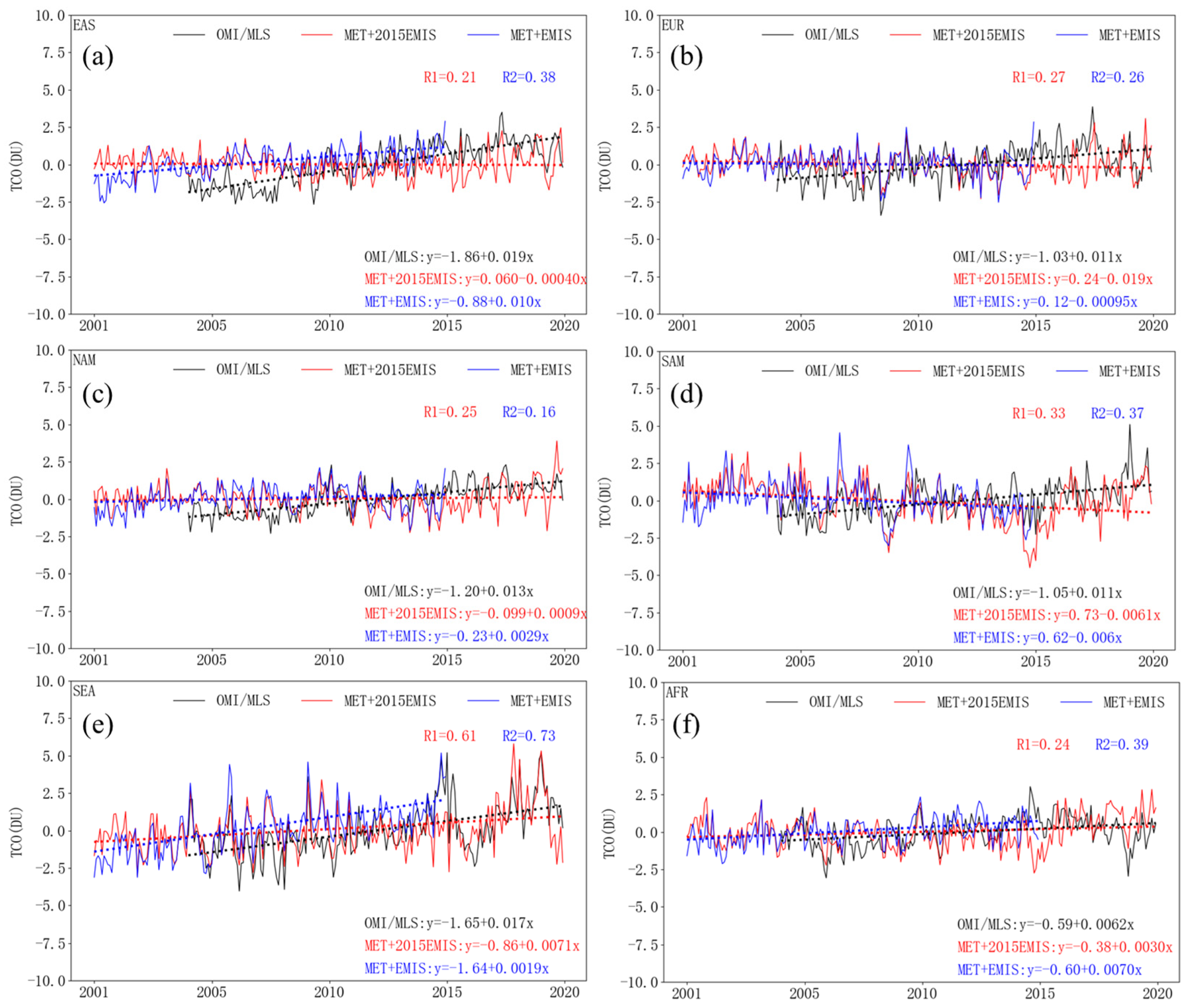
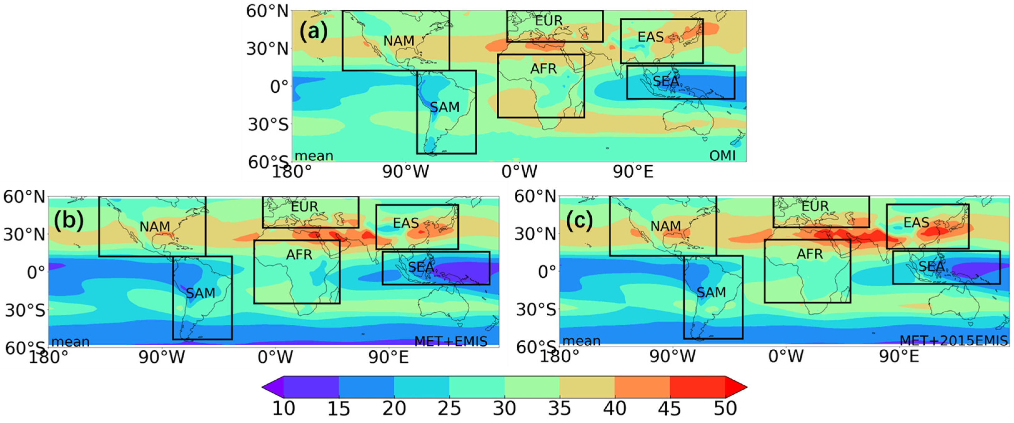
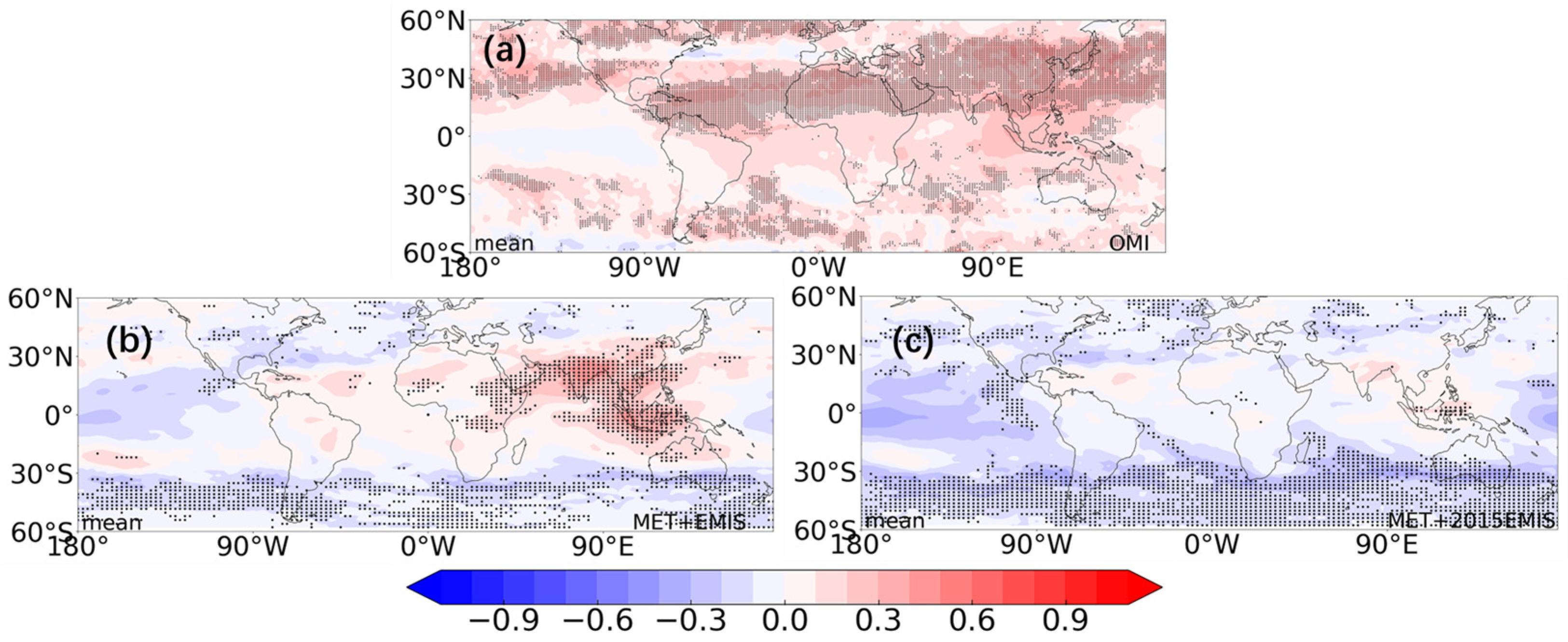
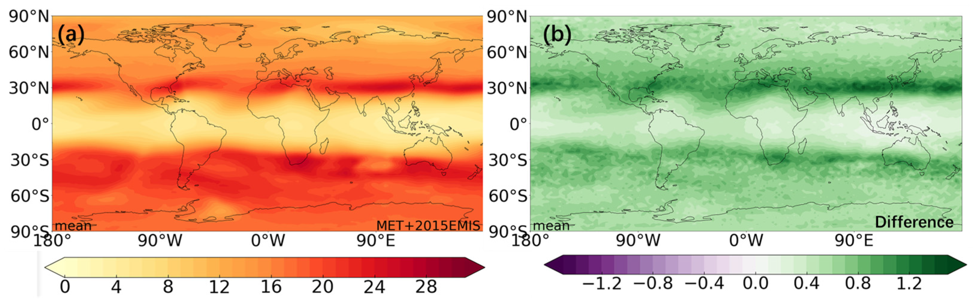
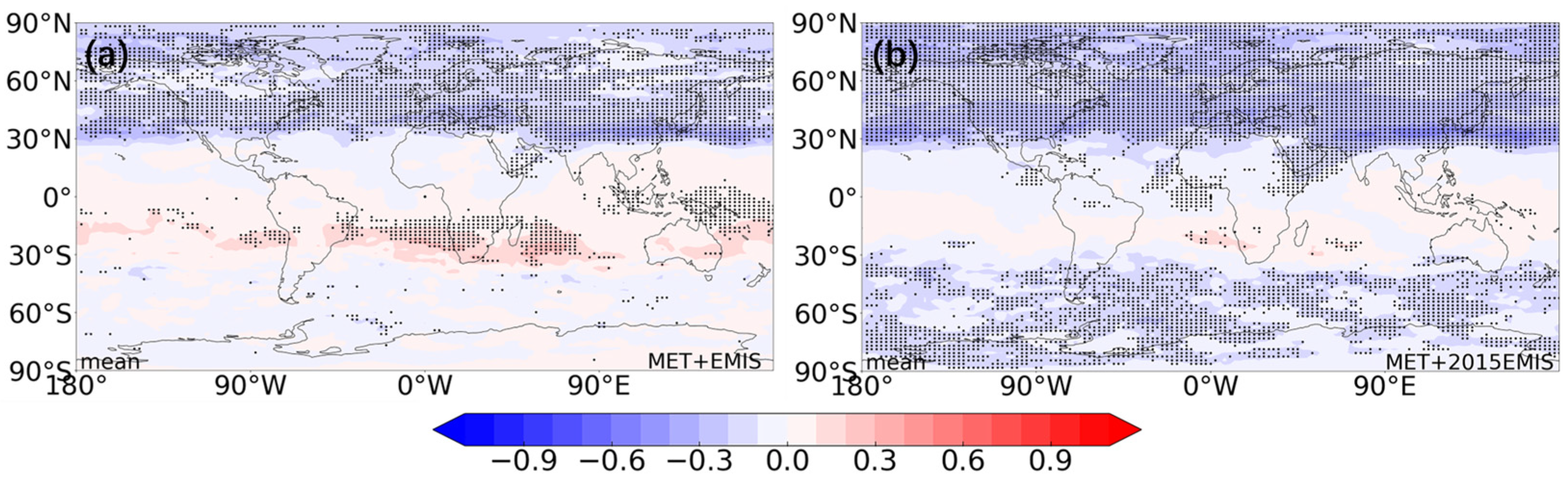
3.1. Distribution and Trend of Tropospheric Column Ozone

Figure 1 shows multi-year mean spatial distribution of TCO based on OMI/MLS satellite data, simulated results of case MET+EMIS and case MET+2015EMIS. In Figure 1a, it can be found from OMI/MLS satellite data that TCO in the northern hemisphere is higher than southern hemisphere, especially in the south of East Asia and Europe, and the north of Africa with the highest value of more than 40 DU. Over Southeast Asia and South America, TCO is low with the lowest value of less than 20 DU. Figure 1b,c are the MET+EMIS and MET+2015EMIS experiments results, respectively. Multi-year mean of TCO in MET+2015EMIS is higher than in MET+EMIS, due to the fixed emission inventory in year 2015 of case MET+2015EMIS which keeps a higher precursors emission than in case MET+EMIS. And the difference in simulation time length of these two cases also is attributed to the difference in TCO. The simulated TCO values in both two cases are higher than satellite data in East Asia and the south of Europe (~50 DU), and are lower in tropical Pacific Ocean (~15 DU) and south hemisphere (~30 DU), which may be due to the coarse horizontal and vertical resolutions and the accuracy of emission inventory used by simulation experiments. In summary, the comparison of simulated TCO with the OMI/MLS satellite data indicate that the simulated results capture the high values of TCO in the middle latitude of northern hemisphere and the low values in tropical Pacific Ocean well, and can be used in this study. Comparing to the MET+EMIS, the results of MET+2015EMIS are higher than satellite data.
The MK Test and a linear estimator are used to calculate the annual trend of TCO by satellite data and simulated results, as shown in Figure 2. Figure 2a is the trend of TCO in satellite data, which shows an increase year by year in most parts of the world. The increase in the northern hemisphere is stronger than southern hemisphere, and the strongest value of more than 0.3 DU/yr located near 30°N. Figure 2b is the simulated results of case MET+EMIS which used the dynamic emission inventory. The simulated TCO also shows a significant increase from 2001 to 2015 in East Asia and Southeast Asia, indicating that the simulated results capture the trend of TCO in satellite data over East Asia and Southeast Asia well. But in middle and high latitudes above 30°S the simulated results mismatched the week increase in OMI/MLS data. The accuracy of emission inventories in the simulation and the uncertainty in satellite data both contribute to the differences of TCO between satellite data and simulated results. Figure 2c is the result of case MET+2015EMIS with fixed emission inventory in year 2015, and the annual trend of TCO is mainly attribute to the change in meteorological field. The change in meteorological field makes the TCO decrease in various regions of the world, especially in the middle and high latitudes of the southern hemisphere, which has passed the 95% significance test. Over East Asia and Southeast Asia, the increase in Figure 2b becomes weaker in Figure 2c. It indicates the emission of ozone precursors makes the TCO increase over East Asia and Southeast Asia while the change in meteorological field weakened the increase, which also matched the previous study [8,25]. For Southeast Asia, TCO still shows an increase in case MET+2015EMIS, which may result from the increased temperature and humidity from 2005 to 2015 as a consequence of climate change.
In this study, six regions are classified to describe the regional changes in detail: North America (12°N–60°N, 140°W–55°W, NAM), South America (50°S–12°S, 81°W–34.5°W, SAM), Africa (25°S–25°N, 17°W–51°E, AFR), Europe (35°N–60°N, 10°W–66°E, EUR), East Asia (18°N–53°N, 80°E–145°E, EAS) and Southeast Asia (10°S–16°N, 85°E–170°E, SEA). Their locations are shown in Figure 1. The de-seasonal trend of TCO in regional averages are shown in Figure 3 and Table 2. The OMI/MLS data showed a significant increase in these six regions, with the largest value of 0.23 DU/yr in the EAS region, and the smallest value of ~0.07 DU/yr in the AFR region. The model results of case MET+EMIS also show significant increased trends in the NAM, EAS, AFR and SEA regions. But the largest value is SEA (~0.23 DU/yr) and the smallest value is NAM, (~0.03 DU/yr). The annual variability in the SAM and EUR regions is negative but insignificant. In MET+2015EMIS, the annual variation over SEA still is increased, with a value of 0.09 DU/yr, but they turn to insignificant decreases in the NAM, EAS and AFR. This also proved that the increased trend of TCO in the EAS is most affected by the changes in emissions, while it is least affected by emissions in the EUR. In the SEA, the increased TCO due to both the changes in meteorological conditions and emissions.

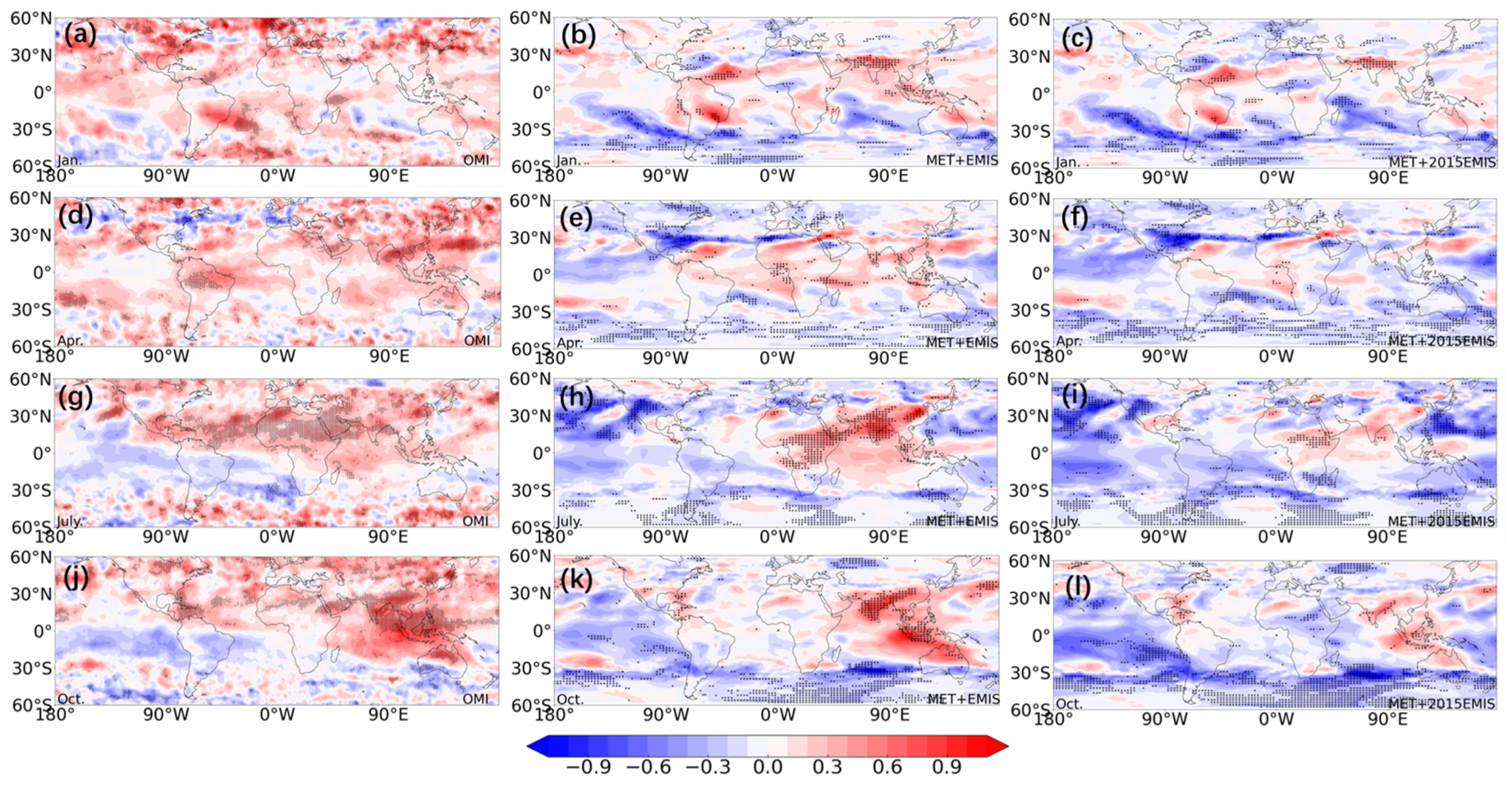
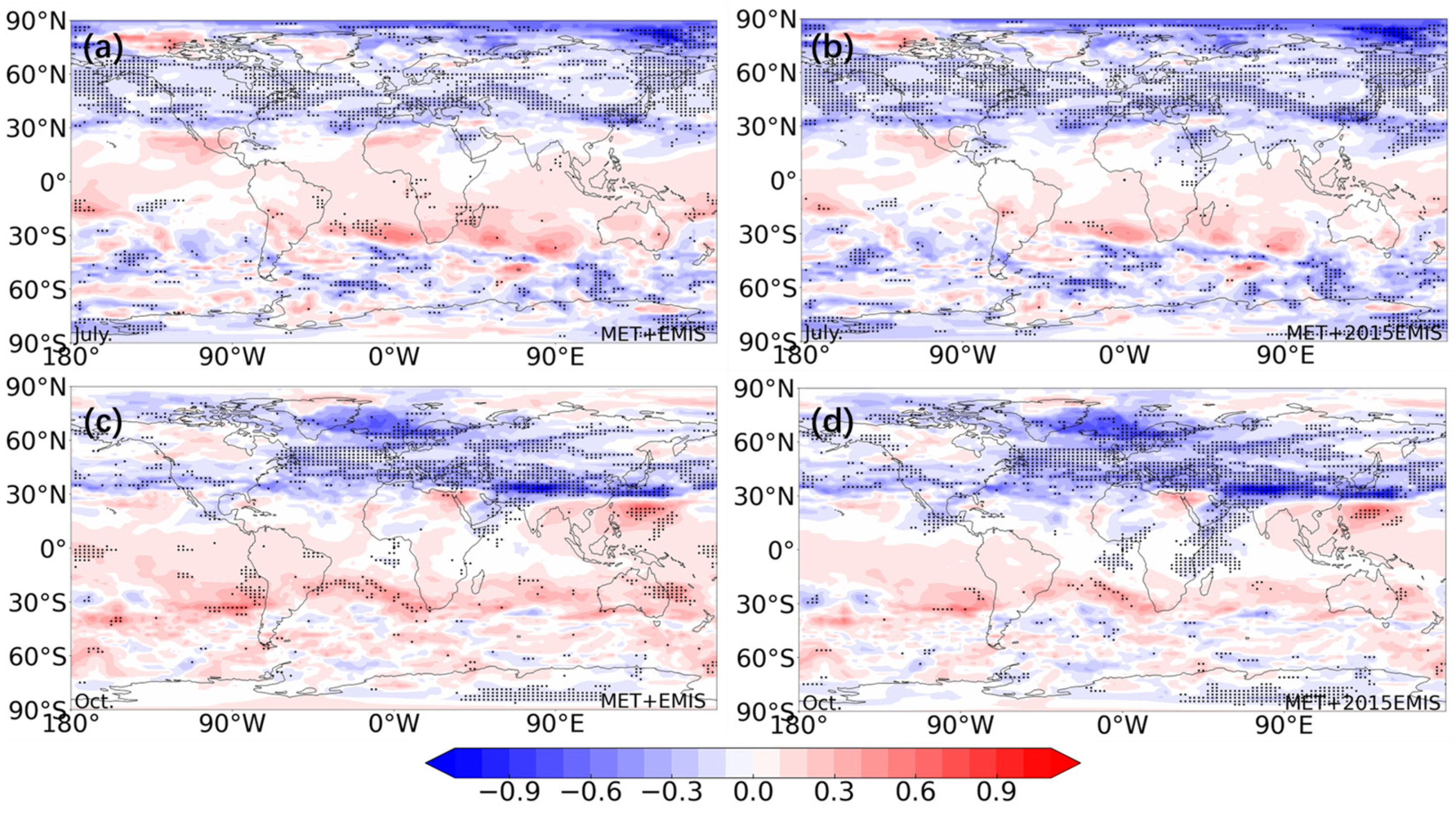
3.2. Seasonal Trend of Tropospheric Column Ozone

We used January, April, July and October to represent winter, spring, summer and autumn, respectively. The distributions of TCO trends in four seasons are calculated, shown in Figure 4 and Table 3. In winter (January, Figure 4a), TCO in OMI/MLS data shows positive trends in most regions, especially in North America, East Asia, Europe and Southeast Asia. The increasing rates in these four regions are more than 0.4 DU/yr. The increase in TCO over Africa is weak, and not significant. In spring (April, Figure 4d), the increase rates in the south of EAS, the west of SEA and the north of SAM are 0.3–0.4 DU/yr, which are significant. Compared with January, the increase in April is weaker in Europe and Africa, but stronger in East Asia, Southeast Asia and north of South America. In summer (July, Figure 4g), TCO is increased in the southeast and northwest of East Asia, Southeast Asia, north of Africa, and south of North America, with the rates of more than 0.3 DU/yr. The MK Test results in the central of Africa, Europe and South America are insignificant. In autumn (October, Figure 4j), there is a significant positive trend in East Asia, and Southeast Asia, with the rates of more than 0.4 DU/yr. The changes in TCO in Africa and South America are insignificant. In summary, TCO in most areas of East Asia and Southeast Asia is increased in four seasons, and the increase rate is the fastest in autumn with a regional value of more than 0.3 DU/yr (shown in Table 3). Over East Asia, the increase rate is the weakest in winter with a regional value of 0.19 DU/yr. Over Southeast Asia, it is the weakest in summer, with a value of 0.15 DU/yr.
The simulated results show that TCO in case MET+EMIS has a significant increase in the middle of East Asia and Southeast Asia in four seasons (Figure 4b,e,h,k), while TCO in case MET+2015EMIS has no obvious change (Figure 4c,f,i,l), indicating that the increase is mainly caused by the change in pollutant emissions. In the central and northern of Africa, southern North America, and central of South America, the change in meteorological field also weakens the increase rate of TCO in winter and spring. It indicates that the changes in emissions in most parts of the world will make TCO increased, while the change in meteorological conditions weaken the increasing rate of TCO, even lead to a significant decrease in most of the southern hemisphere. In summer (July, Figure 4h), the significant increase in TCO covers central of Africa, India and south of China with the value of more than 0.5 DU/yr. In autumn (October, Figure 4k), the significant increase in TCO covers India, south of China, Indonesia, and north of Australia. The comparison between the two simulated results in four seasons indicates that the change in emissions had the greatest impact on the increase in TCO while the change in meteorological conditions weakens the increasing rate, even lead to a decrease in TCO.
In order to quantify the impact of emissions and meteorological fields on the inter-annual variation in TCO, the regional averages of TCO trends are calculated in four seasons (Table 3). The increased rates of TCO are the fastest in EAS and SEA in four seasons based on OMI/MLS data, and the simulated results of case MET+EMIS matches the changes in observed TCO well. In winter (January, Table 3), OMI/MLS data show the significant increasing rates of TCO in NAM, EAS, EUR and SEA are 0.15, 0.19, 0.17 and 0.25 DU/yr on regional average, respectively. The simulated TCO trends also reproduce the increasing rates, but the simulated increasing rates are weaker, and MK Tests in NAM and EUR are insignificant. Similar results are shown in other three seasons. The changes in meteorological conditions lead to insignificant trends of TCO and the variability rate in most regions is below 0.1 DU/yr. In spring (April, Table 3), the change in meteorological field leads to the significant decrease over EAS, SAM and EUR, and the variation rate is approximately 0.05 DU/yr. In summer (July, Table 3), the change in meteorological field only leads to a decrease over EAS with the decreasing rate of 0.06 DU/yr. Based on the regional averages, the comparisons of two simulated results further indicate that the change in emissions had the greatest impact on the increase in TCO while the change in meteorological conditions weaken the increasing rates, even lead to a significant decrease in EAS in spring and summer.

3.3. Impact of Stratospheric Intrusion to the Trend of TCO

Simulated O3S is used to explore the impact of stratospheric intrusion on tropospheric ozone in this study. The distribution of O3S column in the troposphere on multi-year average are shown in Figure 5a. Weak stratospheric intrusion in the equatorial region, and its contribution to TCO is below 10 DU. The tropical region near the equator receives more atmospheric radiation energy, forming an updraft in the Brewer–Dobson circulation, making the stratospheric ozone hardly transported to the troposphere. The stratospheric intrusion is high near 30°N and in the south of 30°S in the southern hemisphere, with the contribution of ~25 DU. It may be affected by the descending branch of the Brewer–Dobson circulation and stratosphere–troposphere exchange in the vicinity of tropical jet stream, which transports more stratospheric ozone into troposphere [26]. At high latitudes, the contribution of stratospheric ozone to TCO in the southern hemisphere is higher than that in the northern hemisphere with the value of more than 15 DU. The reason is that there is more land in the northern hemisphere and the population distribution is denser. At the global scale, the land can be regarded as a heat source, resulting in more updrafts in the northern hemisphere than in the southern hemisphere, making the contribution of stratospheric intrusion in the northern hemisphere lower than that in the southern hemisphere. The faster chemical loss of ozone in the troposphere in the northern hemisphere also attribute to its lower stratospheric contribution. The differences of O3S column in the troposphere in two simulation experiments are shown in Figure 5b. It can be seen that the changes in precursors emission have the greatest impact on O3S in the region at approximately 30°N (S), with a variation of approximately 1.2 DU caused by emissions. The variation in O3S caused by emissions is the smallest in the low-latitude region near the equator, with a variation below 0.4 DU. It indicates that higher emissions of ozone precursors accelerate the photochemical reactions, including the photochemical loss of ozone, which leads to the faster loss of O3S in the troposphere in case MET+2015EMIS.
The trend of O3S column in the troposphere is calculated and shown in Figure 6. In the south of Africa and Australia (0–30°S, Figure 6a), the O3S column in the troposphere shows a significant increase, with an annual rate of less than 0.4 DU/yr, which may be due to the increase in tropopause under warmer climate. In the north of 30°N, the O3S column in the troposphere shows a significant decrease, probably due to the increased water vapor, which accelerates the loss of ozone. The changes in atmosphere circulation also have an influence on the inter-decadal variation in stratospheric intrusion. Comparing the results of the two simulation experiments (Figure 6a,b), it can be seen that the change in meteorological field makes the decrease in O3S column in the troposphere in the north of 30°N more significant, and the change in emissions weakens this decreasing rates. The increase in O3 precursor emissions, especially from aircraft, increases stratospheric ozone and leads to more ozone transported from stratosphere to troposphere, which in turn inhibits the decrease caused by the changes in meteorology.
Due to the significant trends of TCO in summer and autumn from Table 3, the variation rates of O3S column in the troposphere in summer (July) and autumn (October) are calculated using a linear estimator and the MK Test method which shown in Figure 7. In the latitude between 30°S–30°N, stratospheric contributions to TCO are increased in summer and autumn, and the increasing rates are more than 0.2 DU/yr, much higher than annual average in Figure 6. The decreasing rates in the north of 30°N are stronger than the annual average, especially in the north of China with more than 0.5 DU/yr in autumn. Changes in meteorological conditions will significantly affect the contribution of this region, resulting in significant inter-decadal variability of stratospheric contributions in these regions. At low latitudes, the increased height of tropopause may contribute to the increased stratospheric input, which leads to an increase in stratospheric contributions to TCO. At middle and high latitudes, the changes in temperature and relative humidity may contribute to the change in O3S column in the troposphere. The rising temperature may accelerate the chemical process of ozone and the loss of O3S. In addition, an increase in temperature may also increase the water vapor content in the atmosphere, which may lead to increased ozone loss, following the reactions below:
O3 + hv → O2 + O (D1)
O (D1) + H2O → 2OH
Comparing the two simulations results, the change in emissions weakens the decreasing rates and enhances the increasing rates significantly with the similar reasons in annual trend of Figure 6.

4. Conclusions

Based on the OMI/MLS satellite data and the simulation experiments of CESM2 model, the distributions of trends and seasonal changes in TCO in the recent two decades are explored, and the effects of meteorological field and emission on tropospheric ozone trend are also compared and quantified. Based on the simulated variable of O3S, the influence of stratospheric intrusion on tropospheric ozone is quantitatively analyzed.
The increase in TCO in the northern hemisphere is stronger than that in the southern hemisphere, which has the strongest rate value of 0.3 DU/yr near 30°N. The increasing rates over North America, East Asia, South America, Africa, Europe, and South of East Asia are 0.15, 0.23, 0.13, 0.07, 0.13 and 0.21 DU/yr, respectively, and the value all passed the MK Test. In four seasons, the increasing rates are highest in autumn, especially over North America, East Asia, Europe and South of East Asia with rate values of 0.20, 0.31, 0.17, and 0.32 DU/yr, respectively. The simulated results capture the distribution and seasonal changes in TCO trends in satellite data well, especially over East Asia and South of East Asia. The simulated experiments indicate that the change in ozone precursors emissions had the greatest impact on the increase in TCO while the change in meteorological conditions weaken the increasing rates, even lead to the significant decrease over East Asia in April and July.
The contribution of stratospheric ozone on TCO in the tropical troposphere is the lowest, with a value of below 10 DU. At approximately the latitude of 30°N/S, the stratospheric contribution on TCO is high which affected by the descending branch of the Brewer–Dobson circulation and stratosphere–troposphere exchange in the vicinity of tropical jet stream, approximately 25 DU. In 30°S~30°N, the stratospheric contribution shows a weak increase, with an annual variation rate of below 0.4 DU/yr, while it shows a significant decrease in the north of 30°N. The changes in meteorological conditions under climate change contribute to the trend of stratospheric contributions on TCO. The change in emissions weakens the decreasing rates and enhances the increasing rates from climate change significantly. The trends of stratospheric contributions on TCO partly explain the trends of TCO which are mostly affected by changes in emissions. To control the increasing TCO, actions to reduce emissions are urgently needed, especially over East Asia and Southeast Asia.
One limitation of our study is the time duration of satellite data, from 2005 to 2020. Before 2005, it is TOMS. Different data sources may increase the uncertainty of TCO trends. In the future, we will try to use more reliable data to obtain clearer results.

Author Contributions

Conceptualization, X.H.; Methodology, Y.Z. and X.L.; Validation, X.H.; Formal analysis, Y.Z.; Resources, X.H.; Data curation, X.L.; Writing—original draft, Y.Z. and X.H.; Writing—review & editing, X.H. and J.L.; Visualization, Y.Z. and J.L.; Supervision, X.H. and J.L.; Project administration, X.H. All authors have read and agreed to the published version of the manuscript.

Funding

This research was funded by the National Key Research and Development Program of China (Grant No., 2022YFC3701204) and the Key Laboratory of Atmospheric Chemistry, China Meteorological Administration (LAC/CMA, Grant No., 2023B05).

Data Availability Statement

Data are contained within the article.

Acknowledgments

Numerical calculations in this paper have been performed on the high-performance computing system at the High-Performance Computing Center, Nanjing University of Information Science and Technology. This paper was edited by Nikola Labovic and reviewed by three anonymous referees.

Conflicts of Interest

The authors declare no conflict of interest.

References

  1. Li, G.; Tan, Y.K.; Li, C.Y.; Chen, S.C.; Bai, T.; Yang, D.Y.; Zhang, Y. The distribution characteristics of total ozone and its relationship with stratospheric temperature during boreal winter in the recent 30 years. Chin. J. Geophys. 2015, 58, 1475–1491. (In Chinese) [Google Scholar]
  2. Wild, O. Modelling the global tropospheric ozone budget: Exploring the variability in current models. Atmos. Chem. Phys. 2007, 7, 2643–2660. [Google Scholar]
  3. Gaudel, A.; Cooper, O.R.; Ancellet, G.; Barret, B.; Boynard, A.; Burrows, J.P.; Clerbaux, C.; Coheur, P.F.; Cuesta, J.; Cuevas, E.; et al. Tropospheric Ozone Assessment Report: Present-day distribution and trends of tropospheric ozone relevant to climate and global atmospheric chemistry model evaluation. Elem. Sci. Anthr. 2018, 6, 39. [Google Scholar]
  4. Mehmood, T.; Hassan, M.A.; Li, X.H.; Ashraf, A.; Rehman, S.; Bilal, M.; Obodo, R.M.; Mustafa, B.; Shaz, M.; Bibi, S.; et al. Mechanism behind Sources and Sinks of Major Anthropogenic Greenhouse Gases. In Climate Change Alleviation for Sustainable Progression: Floristic Prospects and Arboreal Avenues as a Viable Sequestration Tool; Dervash, M.A., Wani, A.A., Eds.; CRC Press: Boca Raton, FL, USA, 2022; pp. 114–150. [Google Scholar]
  5. Tian, H.; Ren, W.; Tao, B.; Chappelka, A.; Wang, X.; Pan, S.; Yang, J.; Liu, J.; Ben, S.; Jerry, M.; et al. Impacts of tropospheric ozone and climate change on net primary productivity and net carbon exchange of China’s forest ecosystems. Glob. Ecol. Biogeogr. 2011, 20, 391–406. [Google Scholar]
  6. Wang, T.; Xue, L.; Brimblecombe, P.; Lam, Y.F.; Li, L.; Zhang, L. Ozone pollution in China: A review of concentrations, meteorogical influences, chemical precursors, and effects. Sci. Total Environ. 2016, 575, 1582–1596. [Google Scholar] [PubMed]
  7. Ziemke, J.R.; Oman, L.D.; Strode, S.A.; Douglass, A.R.; Taylor, S.L. Trends in global tropospheric ozone inferred from a composite record of toms/omi/mls/omps satellite measurements and the merra-2 gmi simulation. Atmos. Chem. Phys. 2019, 19, 3257–3269. [Google Scholar]
  8. Zhang, Y.; Cooper, O.R.; Gaudel, A.; Philippe, N.; Ogino, S.; Anne, M.T.; West, J.J. Tropospheric ozone change from 1980 to 2010 dominated by equatorward redistribution of emissions. Nat. Geosci. 2016, 9, 875–879. [Google Scholar]
  9. Ziemke, J.R.; Chandra, S.; Bhartia, P.K. A 25-year data record of atmospheric ozone in the Pacific from Total Ozone Mapping Spectrometer (TOMS)cloud slicing: Implications for ozone trends in the stratosphere and troposphere. J. Geophys. Res. Atmos. 2005, 110, D15105. [Google Scholar]
  10. Lal, D.M.; Ghude, S.D.; Patil, S.D.; Kulkarni, S.H.; Jena, C.; Tiwari, S.; Srivastava, M.K. Tropospheric ozone aerosol long-term trends over the Indo-Gangetic Plain (IGP), India. Atmos. Res. 2012, 116, 82–92. [Google Scholar]
  11. Kulkarni, P.S.; Bortoli, D.; Salgado, R.; Antón, M.; Costa, M.J.; Silva, A.M. Tropospheric ozone variability over the Iberian Peninsula. Atmos. Environ. 2011, 45, 174–182. [Google Scholar]
  12. Kulkarni, P.S.; Jain, S.L.; Ghude, S.D.; Arya, B.C.; Dubey, P.K.; Shahnawaz. On some aspects of tropospheric ozone variability over the Indo-Gangetic (IG) basi, India. Int. J. Remote Sens. 2009, 30, 4111–4122. [Google Scholar]
  13. Lin, M.; Horowitz, L.W.; Payton, R.; Fiore, A.M.; Tonnesen, G. US surface ozone trends and extremes from 1980 to 2014: Quantifying the roles of rising Asian emissions, domestic controls, wildfires, and climate. Atmos. Chem. Phys. 2017, 17, 2943–2970. [Google Scholar]
  14. Oltmans, S.J.; Lefohn, A.S.; Shadwick, D.; Harris, J.M.; Scheel, H.E.; Galbally, I.; Tarasick, D.W.; Johnson, B.J.; Brunke, E.G.; Claude, H.; et al. Recent tropospheric ozone change—A pattern dominated by slow or no growth. Atmos. Environ. 2013, 67, 331–351. [Google Scholar]
  15. Parrish, D.D.; Law, K.S.; Staehelin, J.; Derwent, R.; Cooper, O.R.; Tanimoto, H.; Volz-Thomas, A.; Gilge, S.; Scheel, H.E.; Steinbacher, M.; et al. Long-term changes in lower tropospheric baseline ozone concentrations at northern mid-latitudes. Atmos. Chem. Phys. 2012, 12, 13881–13931. [Google Scholar]
  16. Parrish, D.D.; Derwent, R.G.; Staehelin, J. Long-term changes in northern mid-latitude tropospheric ozone concentrations: Synthesis of two recent analyses. Atmos. Environ. 2021, 248, 118–227. [Google Scholar]
  17. Cooper, O.R.; Parrish, D.D.; Ziemke, J.; Balashow, N.V.; Cupeiro, M. Global distribution and trends of tropospheric ozone: An observation-based review. Elem. Sci. Anthr. 2014, 2, 2–29. [Google Scholar]
  18. Anet, J.G.; Steinbacher, M.; Gallardo, L.; Patricio, A.; Álvarez, V.; Emmenegger, L.; Buchmann, B. Surface ozone in the southern hemisphere: 20 years of data from a site with a unique setting in El Tololo, Chile. Atmos. Chem. Phys. 2017, 17, 6477–6492. [Google Scholar]
  19. Lu, X.; Zhang, L.; Zhao, Y.; Daniel, J.J.; Hu, Y.; Hu, L.; Gao, M.; Liu, X.; Petropavlovskikh, I.; Audra, M.B.; et al. Surface and tropospheric ozone trends in the Southern Hemisphere since 1990: Possible linkages to poleward expansion of the Hadley circulation. Sci. Bull. 2019, 64, 400–409. [Google Scholar]
  20. Hassan, M.A.; Faheem, M.; Mehmood, T.; Yin, Y.; Liu, J. Assessment of meteorological and air quality drivers of elevated ambient ozone in Beijing via machine learning approach. Environ. Sci. Pollut. Res. 2023, 30, 104086–104099. [Google Scholar]
  21. Ziemke, J.R.; Chandra, S.; Duncan, B.N.; Froidevaux, L.; Bhartia, P.F.; Levelt, P.F.; Waters, J.W. Tropospheric ozone determined from Aura OMI and MLS: Evaluation of measurements and comparison with the Global Modeling Initiative Chemical Transport Model. J. Geophys. Res. 2006, 111, 193–203. [Google Scholar]
  22. Esterby, S.R. Review of methods for the detection and estimation of trends with emphasis on water quality applications. Hydrol. Process. 1996, 10, 127–149. [Google Scholar]
  23. Mann, H.B. Non-parametric tests against trend. Econometrica 1945, 13, 163–171. [Google Scholar]
  24. Lv, X.; Hou, X.W.; Lu, W. Numerical simulation of the impact of intercontinental transmission on tropospheric ozone in China. China Environ. Sci. 2021, 41, 537–547. (In Chinese) [Google Scholar]
  25. Sicard, P.; Agathokleous, E.; Anenberg, S.C.; Marco, A.D.; Paoletti, E.; Calatayud, E. Trends in urban air pollution over the last two decades: A global perspective. Sci. Total Environ. 2023, 858, 160064. [Google Scholar]
  26. Tian, H.; Tian, W.; Luo, J.; Zhang, J.; Yang, Q.; Huang, Q. Characteristics of Water Vapor Distribution and Variation in Upper Troposphere and Lower Stratosphere over Qinghai-Xizang Plateau. Plateau Meteorol. 2014, 33, 1–13. (In Chinese) [Google Scholar]
Figure 1. Multi-year mean spatial distribution of tropospheric column ozone (TCO) (DU) based on OMI/MLS satellite data ((a), 2005–2020), simulated results of case MET+EMIS ((b), 2001–2015) and case MET+2015EMIS ((c), 2001–2020).
Remotesensing 15 05293 g001
Figure 2. Annual trend of TCO (DU/yr) in OMI/MLS satellite data ((a), 2005–2020), simulated results of case MET+EMIS ((b), 2001–2015) and case MET+2015EMIS ((c), 2001–2020). The regions covered by black spot means the significance passed the MK trend test with a confidence interval of 95%.
Remotesensing 15 05293 g002
Figure 3. The regional averages of de-seasonal trend of TCO (DU) in OMI/MLS satellite data and simulated results over the EAS (a), EUR (b), NAM (c), SAM (d), SEA (e), and AFR (f) regions. The solid line is the de-seasonal monthly values of TCO (DU), and the dotted line is the linear fitting results. Black represents OMI/MLS data, red represents simulated results of case MET+2015EMIS, blue represents simulated results of case MET+EMIS. R1 is the correlation coefficient between OMI/MLS and MET+2015EMIS, while R2 is the correlation coefficient between OMI/MLS and MET+EMIS.
Remotesensing 15 05293 g003
Figure 4. The distribution of TCO trends (DU/yr) in January (ac), April (df), July (gi) and October (jl), based on OMI/MLS satellite data (left panels), case MET+EMIS results (middle panels), and case MET+2015EMIS results (right panels). The regions covered by black spot means the significance has passed the MK Test with a confidence interval of 95%.
Remotesensing 15 05293 g004
Figure 5. The spatial distribution of O3S (DU) column in the troposphere on multi-year average of case MET+EMIS (a) and the difference between the two simulated results ((b), MET+EMIS minus MET+2015EMIS).
Remotesensing 15 05293 g005
Figure 6. Annual trend distribution of simulated tropospheric column O3S (DU/yr) in the case MET+EMIST (a) and case MET+2015 EMIS (b). The regions covered by black spots indicate the significance has passed the MK Test with a confidence interval of 95%.
Remotesensing 15 05293 g006
Figure 7. The trend distribution of O3S column in the troposphere in July (a,b) and October (c,d). The left panels are the simulated results of case MET+EMIS, and the right panels are case MET+2015EMIS. The regions covered by black spot means the significance has passed the MK Test with a confidence interval of 95%.
Remotesensing 15 05293 g007
Table 1. Experimental settings.
EXPMET+EMISMET+2015EMIS
ModelCESM2.2.0CESM2.2.0
Year2001~20152001~2020
EmissionDynamic emission inventoryFixed emission inventory, 2015
Resolution1.9° × 2.5°1.9° × 2.5°
Level5656
ComponentFCSDFCSD
Chemical mechanismtroposphere/stratosphere chemistry with simplified VBS-SOA, MOZART-TS1
Spin-up20002000
Table 2. Annual variation rates and MK trend test results of each region.
Slope (DU/yr)NAMEASSAMAFREURSEA
OMI/MLS0.15 *0.23 *0.13 *0.07 *0.13 *0.21 *
MET+EMIS0.03 *0.13 *−0.070.08 *−0.010.23 *
MET+2015EMIS0.01−0.01−0.07 *0.04−0.02 *0.09 *
Note: The star (*) in the table indicates that it has passed the MK Test with a confidence of 95%. The red font indicated positive trend and the blue font indicated negative trend. The unit is DU per year (DU/yr).
Table 3. Annual variability rates and MK trend test results of each region.
Slope (DU/yr)NAMEASSAMAFREURSEA
Jan.OMI0.15 *0.19 *0.230.080.17 *0.25 *
MET+EMIS0.050.10 *0.020.12 *0.020.22 *
MET+2015EMIS0.000.04−0.100.050.040.12
Apr.OMI0.11 *0.23 *0.12 *0.060.100.20 *
MET+EMIS0.000.09−0.12 *0.13 *0.020.18 *
MET+2015EMIS−0.07−0.06 *−0.07 *0.05−0.05 *0.07
Jul.OMI0.18 *0.25 *0.090.060.090.15 *
MET+EMIS−0.060.22 *−0.080.22 *−0.060.20 *
MET+2015EMIS0.02−0.06 *−0.060.07−0.030.02
Oct.OMI0.20 *0.31 *0.100.030.17 *0.32 *
MET+EMIS0.080.15 *0.16 *0.040.020.28 *
MET+2015EMIS0.070.060.15 *0.040.040.09
Note: The star (*) in the table indicates that it has passed the MK Test with a confidence of 95%. The red font indicated positive trend and the blue font indicated negative trend. The unit is DU per year (DU/yr).
Disclaimer/Publisher’s Note: The statements, opinions and data contained in all publications are solely those of the individual author(s) and contributor(s) and not of MDPI and/or the editor(s). MDPI and/or the editor(s) disclaim responsibility for any injury to people or property resulting from any ideas, methods, instructions or products referred to in the content.

