
A Gridless DOA Estimation Method for Sparse Sensor Array


Abstract
:1. Introduction
- (1)
- Combined with unsupervised learning, a DOA estimation method for sparse sensor arrays is first proposed. Our proposed method combines the advantages of DL and can reduce the problem of computational complexity to some extent by using the data-driven approach.
- (2)
- We introduce ResNet and combine it with unsupervised learning. The proposed method is a good solution when facing the dilemma that labeled datasets in DOA estimation are hard to obtain. Due to the characteristics of the residual network itself, the network structure proposed in this paper can circumvent gradient disappearance and gradient explosion and can solve the overfitting of the deep network.
- (3)
- We took some complex environments into consideration, such as low SNRs and few snapshots. Methods are given on how to train the network using data containing such errors.
2. Model and Cost Function
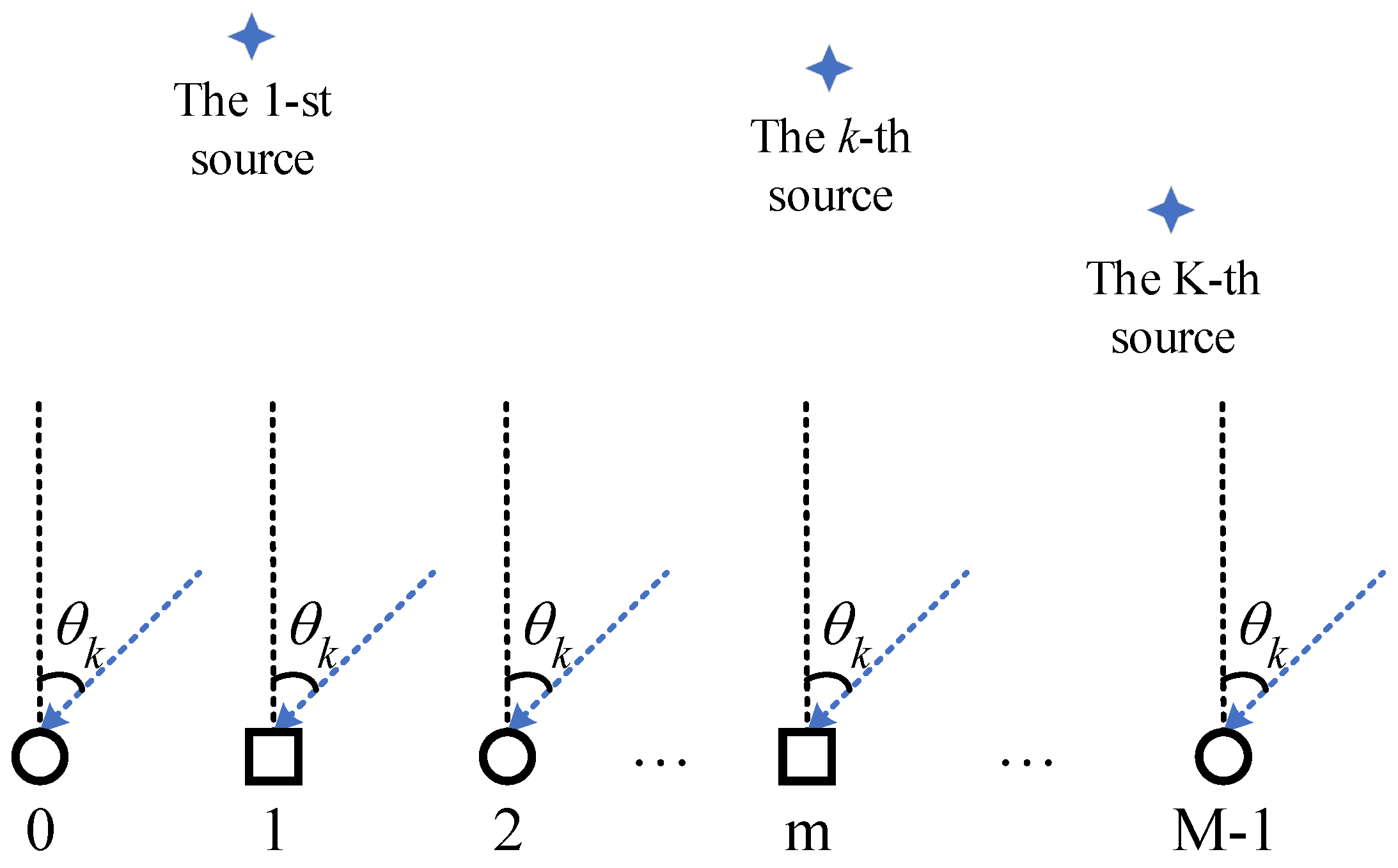
2.1. Model
2.2. The Cost Function of Network Training
3. Deep Networks for DOA Estimation
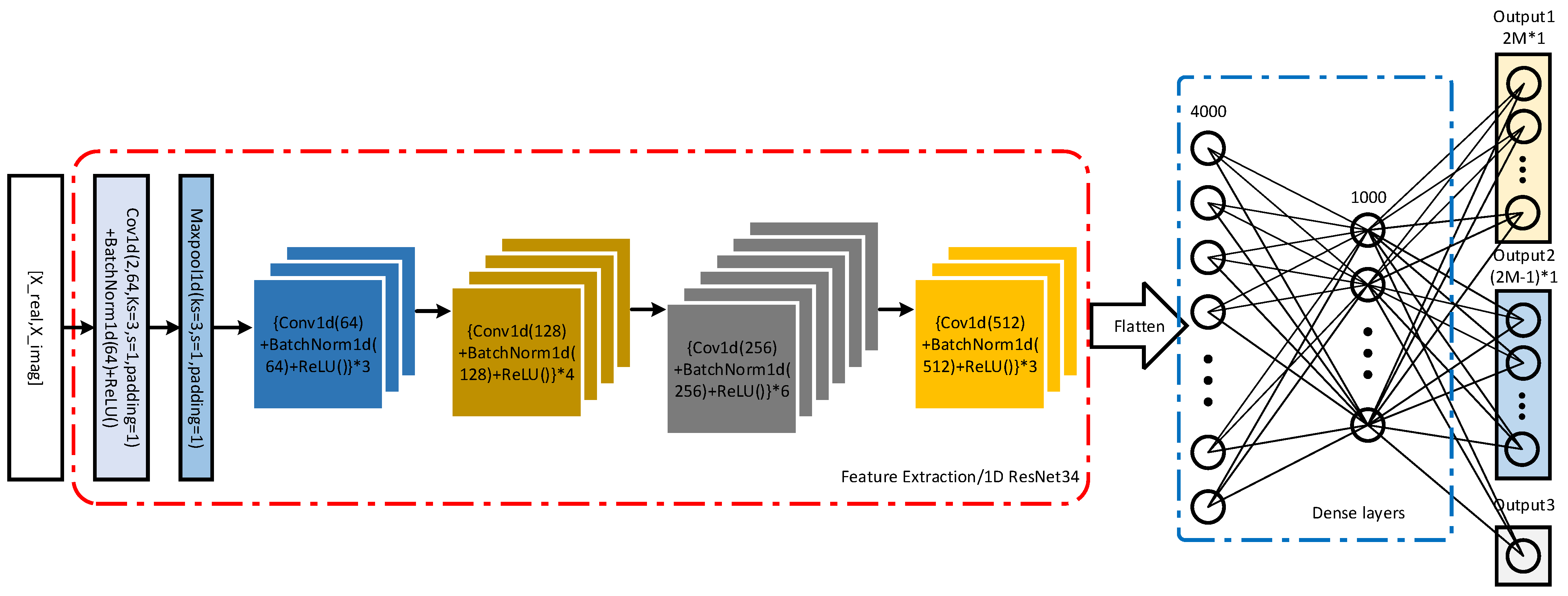
3.1. Network Structure
3.2. DOA Estimation
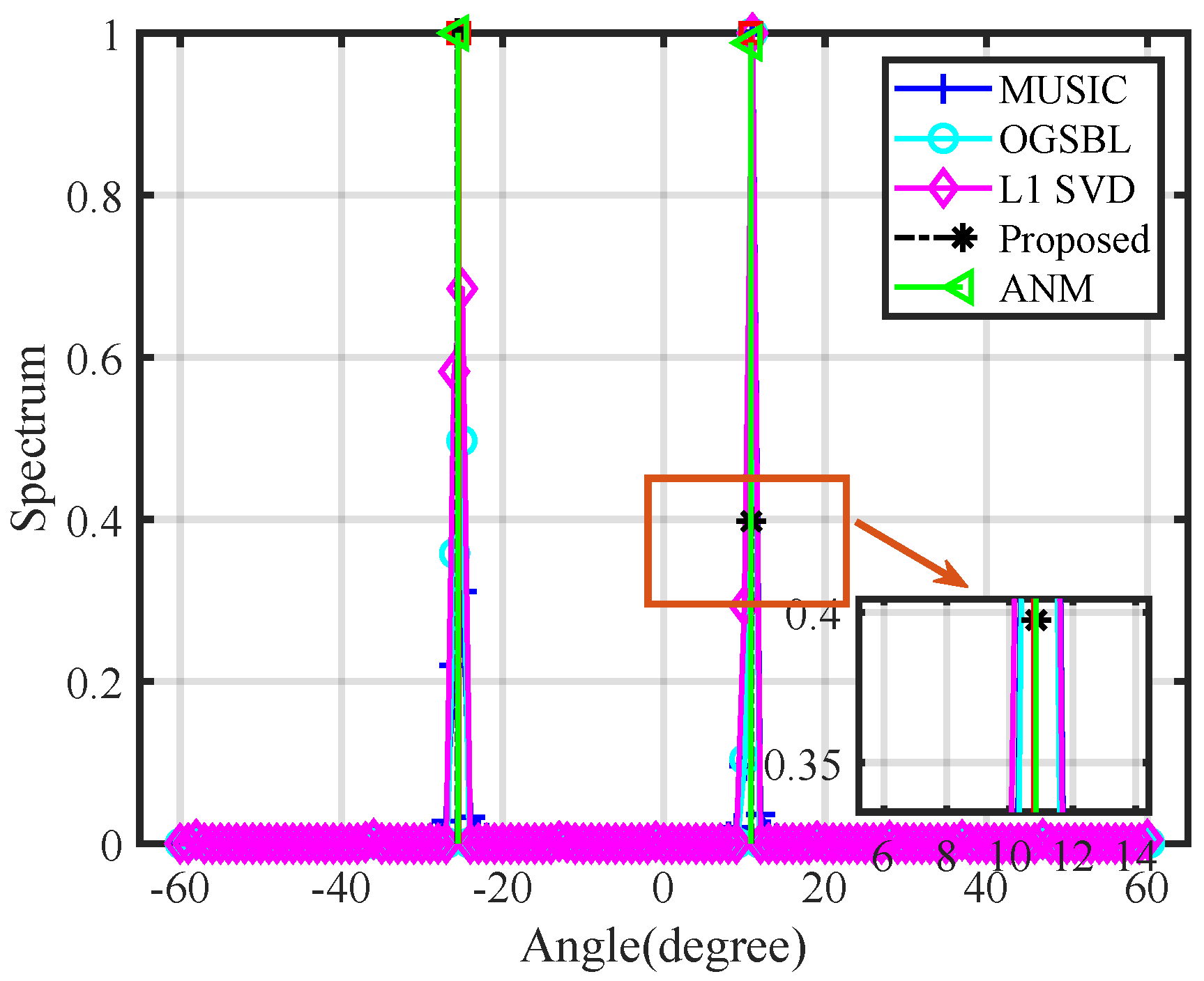
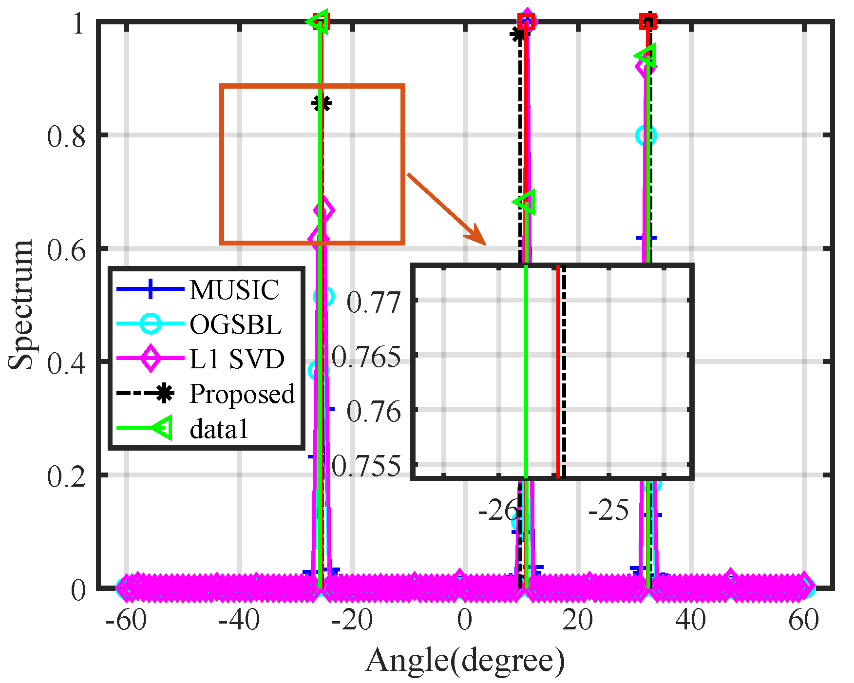
4. Simulations
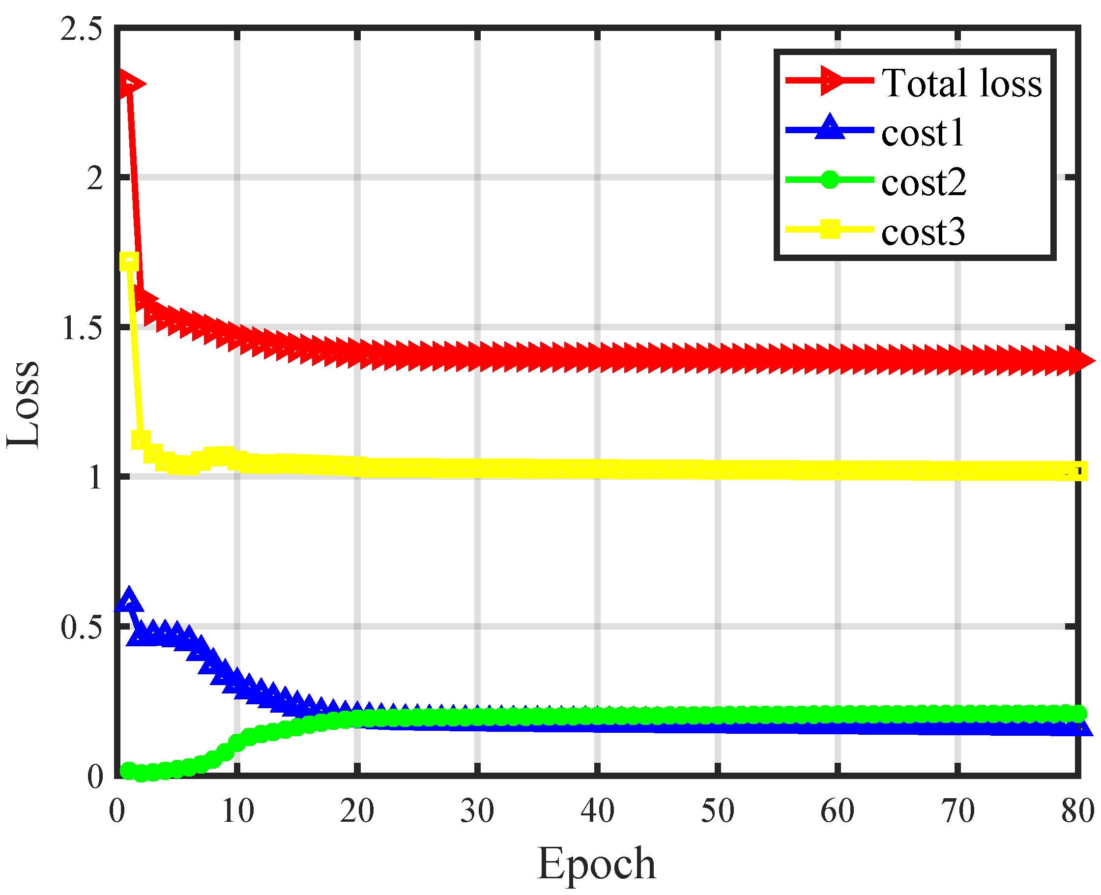
4.1. Network Training
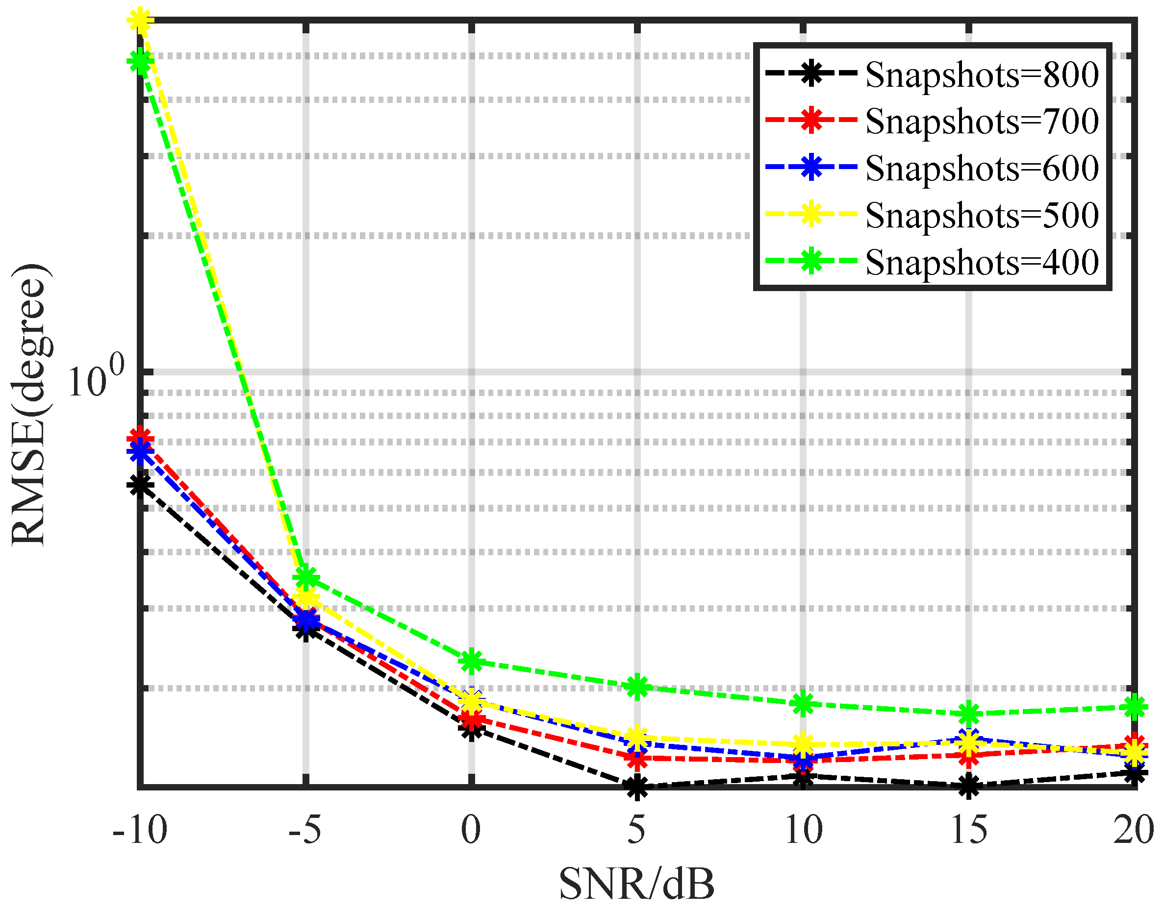
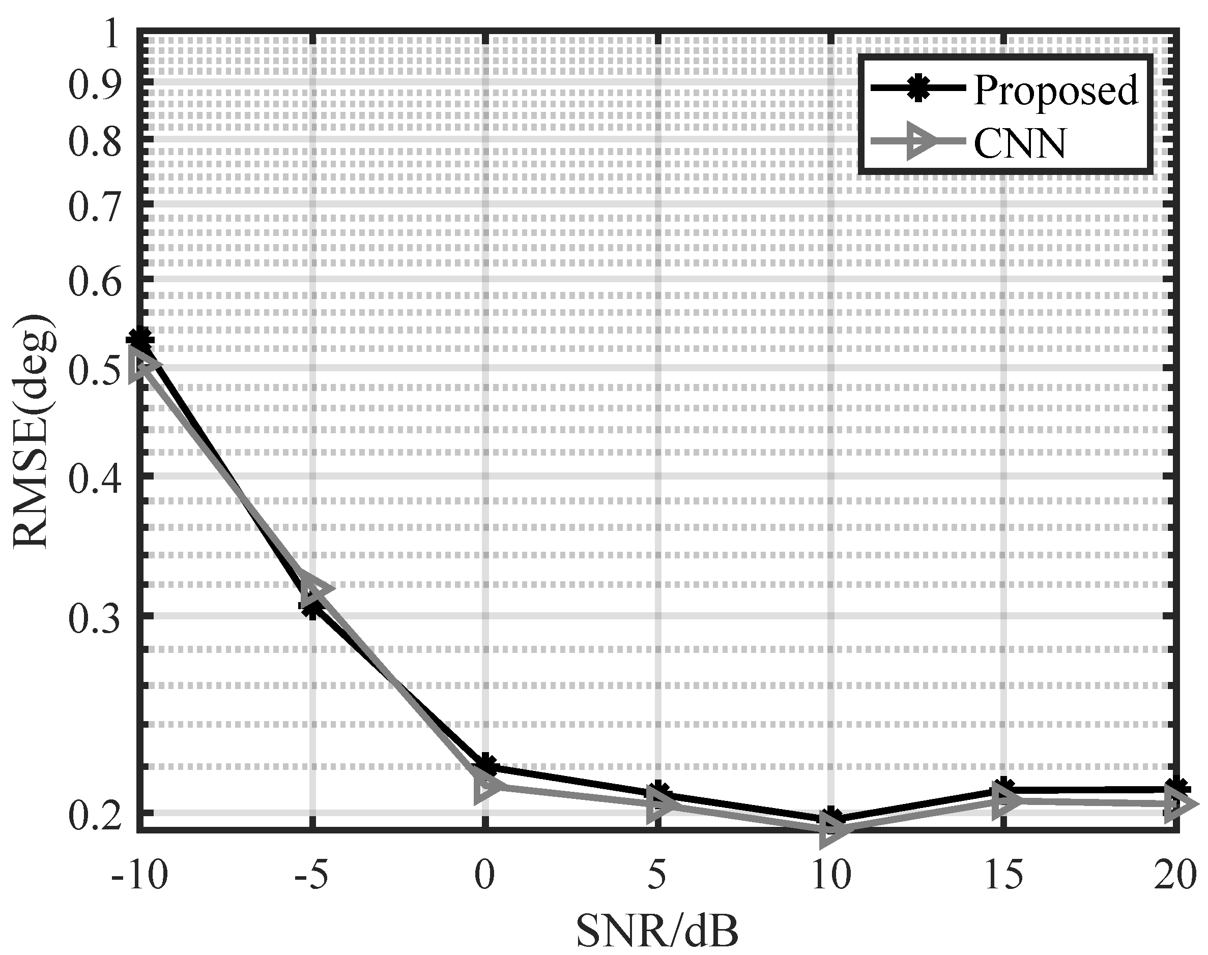
4.2. Performance Analysis
4.3. Computational Complexity Analysis
4.4. Adaptability of Different Network Architectures
5. Conclusions
Author Contributions
Funding
Data Availability Statement
Acknowledgments
Conflicts of Interest
References
- Huang, Q.; Fang, W. A Deep Learning Method for DOA Estimation with Covariance Matrices in Reverberant Environments. Appl. Sci. 2022, 12, 4278. [Google Scholar] [CrossRef]
- Yuan, Y.; Wu, S.; Wu, M.; Yuan, N. Unsupervised learning strategy for direction-of-arrival estimation network. IEEE Signal Process. Lett. 2021, 28, 1450–1454. [Google Scholar] [CrossRef]
- Guo, M.; Zhang, Y.D.; Chen, T. DOA estimation using compressed sparse array. IEEE Trans. Signal Process. 2018, 66, 4133–4146. [Google Scholar] [CrossRef]
- Schmidt, R. Multiple emitter location and signal parameter estimation. IEEE Trans. Antennas Propag. 1986, 34, 276–280. [Google Scholar] [CrossRef]
- Vallet, P.; Mestre, X.; Loubaton, P. Performance analysis of an improved MUSIC DoA estimator. IEEE Trans. Signal Process. 2015, 63, 6407–6422. [Google Scholar] [CrossRef]
- Gao, F.; Gershman, A.B. A generalized ESPRIT approach to direction-of-arrival estimation. IEEE Signal Process. Lett. 2005, 12, 254–257. [Google Scholar] [CrossRef]
- Haardt, M.; Nossek, J.A. Unitary ESPRIT: How to obtain increased estimation accuracy with a reduced computational burden. IEEE Trans. Signal Process. 1995, 43, 1232–1242. [Google Scholar] [CrossRef]
- Zheng, G.; Chen, B.; Yang, M. Unitary ESPRIT algorithm for bistatic MIMO radar. Electron. Lett. 2012, 48, 179–181. [Google Scholar] [CrossRef]
- Chen, J.; Zhang, T.; Li, J.; Chen, X. Joint Sensor Failure Detection and Corrupted Covariance Matrix Recovery in Bistatic MIMO Radar With Impaired Arrays. IEEE Sens. J. 2019, 19, 5834–5842. [Google Scholar] [CrossRef]
- Lin, B.; Liu, J.; Xie, M.; Zhu, J. Direction-of-Arrival Tracking via Low-Rank Plus Sparse Matrix Decomposition. IEEE Antennas Wirel. Propag. Lett. 2015, 14, 1302–1305. [Google Scholar] [CrossRef]
- Das, A. A Bayesian Sparse-Plus-Low-Rank Matrix Decomposition Method for Direction-of-Arrival Tracking. IEEE Sens. J. 2017, 17, 4894–4902. [Google Scholar] [CrossRef]
- Liu, Q.; Gu, Y.; So, H.C. DOA Estimation in Impulsive Noise via Low-Rank Matrix Approximation and Weakly Convex Optimization. IEEE Trans. Aerosp. Electron. Syst. 2019, 55, 3603–3616. [Google Scholar] [CrossRef]
- Donoho, D.L. Compressed sensing. IEEE Trans. Inf. Theory 2006, 52, 1289–1306. [Google Scholar] [CrossRef]
- Malioutov, D.; Cetin, M.; Willsky, A.S. A sparse signal reconstruction perspective for source localization with sensor arrays. IEEE Trans. Signal Process. 2005, 53, 3010–3022. [Google Scholar] [CrossRef]
- Yang, Z.; Xie, L.; Zhang, C. Off-grid direction of arrival estimation using sparse Bayesian inference. IEEE Trans. Signal Process. 2012, 61, 38–43. [Google Scholar] [CrossRef]
- Chen, P.; Cao, Z.; Chen, Z.; Wang, X. Off-Grid DOA Estimation Using Sparse Bayesian Learning in MIMO Radar With Unknown Mutual Coupling. IEEE Trans. Signal Process. 2019, 67, 208–220. [Google Scholar] [CrossRef]
- Tang, G.; Bhaskar, B.N.; Shah, P.; Recht, B. Compressed sensing off the grid. IEEE Trans. Inf. Theory 2013, 59, 7465–7490. [Google Scholar] [CrossRef]
- Yang, Z.; Xie, L. On gridless sparse methods for line spectral estimation from complete and incomplete data. IEEE Trans. Signal Process. 2015, 63, 3139–3153. [Google Scholar] [CrossRef]
- Huang, H.; Yang, J.; Huang, H.; Song, Y.; Gui, G. Deep learning for super-resolution channel estimation and DOA estimation based massive MIMO system. IEEE Trans. Veh. Technol. 2018, 67, 8549–8560. [Google Scholar] [CrossRef]
- Ge, S.; Li, K.; Rum, S.N.B.M. Deep learning approach in DOA estimation: A systematic literature review. Mob. Inf. Syst. 2021, 2021, 6392875. [Google Scholar] [CrossRef]
- Wan, L.; Sun, Y.; Sun, L.; Ning, Z.; Rodrigues, J.J. Deep learning based autonomous vehicle super resolution DOA estimation for safety driving. IEEE Trans. Intell. Transp. Syst. 2020, 22, 4301–4315. [Google Scholar] [CrossRef]
- Kase, Y.; Nishimura, T.; Ohgane, T.; Ogawa, Y.; Kitayama, D.; Kishiyama, Y. DOA estimation of two targets with deep learning. In Proceedings of the IEEE 2018 15th Workshop on Positioning, Navigation and Communications (WPNC), Bremen, Germany, 25–26 October 2018; pp. 1–5. [Google Scholar] [CrossRef]
- Papageorgiou, G.K.; Sellathurai, M.; Eldar, Y.C. Deep networks for direction-of-arrival estimation in low SNR. IEEE Trans. Signal Process. 2021, 69, 3714–3729. [Google Scholar] [CrossRef]
- Papageorgiou, G.K.; Sellathurai, M. Fast direction-of-arrival estimation of multiple targets using deep learning and sparse arrays. In Proceedings of the International Conference on Acoustics, Speech and Signal Processing (ICASSP), Barcelona, Spain, 4–8 May 2020; pp. 4632–4636. [Google Scholar] [CrossRef]
- Yang, Z.; Xie, L. On gridless sparse methods for multi-snapshot DOA estimation. In Proceedings of the IEEE International Conference on Acoustics, Speech and Signal Processing (ICASSP), Shanghai, China, 20–25 March 2016; pp. 3236–3240. [Google Scholar] [CrossRef]
- He, K.; Zhang, X.; Ren, S.; Sun, J. Deep residual learning for image recognition. In Proceedings of the IEEE Conference on Computer Vision and Pattern Recognition, Las Vegas, NV, USA, 27–30 June 2016. pp. 770–778. [CrossRef]
- Fang, W.; Yu, D.; Wang, X.; Xi, Y.; Cao, Z.; Song, C.; Xu, Z. A deep learning based mutual coupling correction and DOA estimation algorithm. In Proceedings of the 13th International Conference on Wireless Communications and Signal Processing (WCSP), Changsha, China, 20–22 October 2021. pp. 1–5. [CrossRef]
- Li, P.; Tian, Y. DOA estimation of underwater acoustic signals based on deep learning. In Proceedings of the 2nd International Seminar on Artificial Intelligence, Networking and Information Technology (AINIT), Nanjing, China, 20–22 October 2021; pp. 221–225. [Google Scholar] [CrossRef]
- Cadzow, J.A.; Kim, Y.S.; Shiue, D.C. General direction-of-arrival estimation: A signal subspace approach. IEEE Trans. Aerosp. Electron. Syst. 1989, 25, 31–47. [Google Scholar] [CrossRef]
- Wu, X.; Zhu, W.P.; Yan, J. A Toeplitz covariance matrix reconstruction approach for direction-of-arrival estimation. IEEE Trans. Veh. Technol. 2017, 66, 8223–8237. [Google Scholar] [CrossRef]
- Chen, T.; Shen, M.; Guo, L.; Hu, X. A gridless DOA estimation algorithm based on unsupervised deep learning. Digit. Signal Process. 2023, 133, 103823. [Google Scholar] [CrossRef]
- Yang, Z.; Xie, L. Exact joint sparse frequency recovery via optimization methods. IEEE Trans. Signal Process. 2016, 64, 5145–5157. [Google Scholar] [CrossRef]
- Candès, E.J.; Fernandez-Granda, C. Towards a mathematical theory of super-resolution. Commun. Pure Appl. Math. 2014, 67, 906–956. [Google Scholar] [CrossRef]
- Kingma, D.P.; Ba, J. Adam: A method for stochastic optimization. arXiv 2014, arXiv:1412.6980. [Google Scholar] [CrossRef]
- Rao, B.D.; Hari, K.S. Performance analysis of root-MUSIC. IEEE Trans. Acoust. Speech Signal Process. 1989, 37, 1939–1949. [Google Scholar] [CrossRef]


| Parameters | Value |
|---|---|
| N | 10 |
| M | 16 |
| L | 1000 |
| P | 100 |
| The wavelength | 1 |
| The location of Source 1 | |
| The location of Source 2 | |
| The location of Source 3 |
| Algorithm | MUSIC | rootMUSIC | OGSBL | L1 SVD | ANM | Proposed |
|---|---|---|---|---|---|---|
| Time/s | 0.0025 | 0.0012 | 246.0584 | 2.4271 | 0.5355 | 0.0123 |
| RMSE/ | 0.3637 | 23.7399 | 0.3248 | 0.3637 | 0.1067 | 0.1095 |
Disclaimer/Publisher’s Note: The statements, opinions and data contained in all publications are solely those of the individual author(s) and contributor(s) and not of MDPI and/or the editor(s). MDPI and/or the editor(s) disclaim responsibility for any injury to people or property resulting from any ideas, methods, instructions or products referred to in the content. |
© 2023 by the authors. Licensee MDPI, Basel, Switzerland. This article is an open access article distributed under the terms and conditions of the Creative Commons Attribution (CC BY) license (https://creativecommons.org/licenses/by/4.0/).
Share and Cite
Gao, S.; Ma, H.; Liu, H.; Yang, J.; Yang, Y. A Gridless DOA Estimation Method for Sparse Sensor Array. Remote Sens. 2023, 15, 5281. https://doi.org/10.3390/rs15225281
Gao S, Ma H, Liu H, Yang J, Yang Y. A Gridless DOA Estimation Method for Sparse Sensor Array. Remote Sensing. 2023; 15(22):5281. https://doi.org/10.3390/rs15225281
Chicago/Turabian StyleGao, Sizhe, Hui Ma, Hongwei Liu, Junxiang Yang, and Yang Yang. 2023. "A Gridless DOA Estimation Method for Sparse Sensor Array" Remote Sensing 15, no. 22: 5281. https://doi.org/10.3390/rs15225281
APA StyleGao, S., Ma, H., Liu, H., Yang, J., & Yang, Y. (2023). A Gridless DOA Estimation Method for Sparse Sensor Array. Remote Sensing, 15(22), 5281. https://doi.org/10.3390/rs15225281