Article

First Assessment of Bistatic Geometric Calibration and Geolocation Accuracy of Innovative Spaceborne Synthetic Aperture Radar LuTan-1

1
National Key Laboratory of Microwave Imaging Technology, Aerospace Information Research Institute, Chinese Academy of Sciences, Beijing 100190, China
2
School of Electronic, Electrical and Communication Engineering, University of Chinese Academy of Sciences, Beijing 100049, China
3
China Center for Resources Satellite Data and Application, Beijing 100049, China
*
Author to whom correspondence should be addressed.
Remote Sens. 2023, 15(22), 5280; https://doi.org/10.3390/rs15225280
Submission received: 12 August 2023 / Revised: 13 October 2023 / Accepted: 3 November 2023 / Published: 7 November 2023
(This article belongs to the Special Issue Spaceborne SAR Calibration Technology)

Abstract

:
LuTan-1 (LT-1) is a bistatic synthetic aperture radar (BiSAR) system consisting of two identical L-band SAR satellites. The bistatic mode of LT-1 plays a critical role in generating high-precision digital elevation models (DEMs), which requires precise geometric calibration of initial range and azimuth times for both SARs to ensure the reliability and quality of geolocation. However, existing geometric calibration methods predominantly focus on monostatic SAR systems, with limited literature on slave SAR calibration in bistatic systems. This research addresses this gap by establishing geometric calibration models for both SARs based on signal echo history and the range–Doppler model. The geometric errors are effectively resolved using corner reflector data from Xinjiang, China. Through statistical analysis of LT-1 SAR images acquired between July and November in bistatic mode, this paper has demonstrated range delay accuracy of better than 5 ns and azimuth time accuracy of better than 0.1 ms. This level of precision translates into a positional accuracy better than 0.8 m. The proposed models have been successfully applied to geometric calibration, providing precise geolocation for LT-1, thus enhancing its utility for a wide range of Earth observation applications. This paper is the first endeavor to present the assessment of the geometric calibration and geolocation accuracy of LT-1 and discuss the results of the bistatic geometric calibration of the master and slave SARs in a BiSAR formation.

1. Introduction

Synthetic aperture radar (SAR) technology has revolutionized Earth observation by enabling the acquisition of high-resolution images regardless of temporal and meteorological conditions [1]. However, azimuth time and range time errors stem from intrinsic temporal deviations within the system, leading to geolocation errors exceeding 10 m in azimuth and range directions. These errors typically exhibit a constant character and necessitate detection through geometric calibration [2]. Geometric calibration estimates systematic time errors by comparing SAR image parameters with reference data, such as corner reflectors (CRs) and digital orthophoto maps (DOMs) [3].
The range–Doppler (RD) model is a classical model in geometric calibration. The RD model, initially proposed in [4], utilizes range and Doppler parameters derived from spaceborne SAR data and satellite ephemeris data to derive the three-dimensional coordinates of ground targets. The authors of [5] discuss the solution method for the RD model, enabling precise pixel localization in digital SAR images. Over time, the RD model has undergone refinement by various researchers. For instance, [6] investigates the impact of atmospheric path delay on geometric calibration, while [7] addresses the bistatic azimuth shift and eliminates errors introduced by the start-stop approximation. Furthermore, [8] explores the influence of solid Earth tidal perturbations, and [9] examines the effect of Doppler shift for terrain observation with progressive scan (TOPS) SAR. As a result, the RD model has found extensive application in the geometric calibration and geolocation of advanced SAR satellites such as ERS [10,11], TerraSAR-X [12,13], ALOS/PALSAR [14,15], Sentinel [8,9,16], RADARSAT [17], and Gaofen-3 [18].
Bistatic SAR (BiSAR) is a radar technology that deploys the transmitter and receiver on independent platforms, offering enhanced system performance, increased reliability, and greater operational flexibility  [19,20]. LuTan-1 (LT-1) is a BiSAR system comprising two SAR satellites, LT-1A and LT-1B, which were successfully launched at the Jiuquan Satellite Launch Center in China on 26 January 2022, and 27 February 2022, respectively [21]. Equipped with advanced L-band polarimetric and multichannel SAR payloads, these satellites can capture images in various modes, offering a maximum resolution of 2 m and a wide observation swath of up to 400 km [22]. The LT-1 constellation advances spatial coverage, imaging versatility, and remote sensing capabilities.
The bistatic mode is a crucial mode of LT-1, where LT-1A transmits L-band electromagnetic waves while LT-1A and LT-1B satellites both receive them [23]. The aim is to employ interferometry to generate a digital elevation model (DEM), a three-dimensional representation of a terrain’s surface. DEMs are widely used in various applications, including terrain analysis, hydrological modeling, land planning, and navigation applications [24,25]. The bistatic mode offers advantages such as excellent interferometric quality, shorter DEM generation cycles, and higher DEM accuracy [26]. However, as DEM is a three-dimensional geolocation product, precise two-dimensional planimetric geolocation is crucial before obtaining elevation information.
Additionally, DEM is created through the interferometric processing process, which includes steps like absolute interferometric phase and baseline calibration to detect the precise interferometric phase and baseline [27]. These steps require precise geometric parameters related to the BiSAR system. Incorrect geometric parameters of the BiSAR system result in the erroneous estimation of the interferometric phase and baseline, decreasing DEM accuracy [21].
However, existing geometric calibration models are developed explicitly for monostatic SAR systems. In this case, the SAR transmits and receives electromagnetic signals. However, the slave SAR exclusively receives electromagnetic signals. The spatial separation of the transmitter and receiver in BiSAR poses calibration challenges, and valid bistatic geometric calibration has not been realized. Despite the emergence of several BiSAR systems, such as TanDEM-X [28] and SAOCOM-1 [29], their calibration of slave SAR is mainly conducted during the pursuit monostatic phase, treating the slave SAR as a monostatic SAR for geometric calibration [30,31]. Furthermore, within the bistatic mode of LT-1, a range time synchronization process is implemented, aligning the timeline of the slave SAR with that of the master SAR. This synchronization renders the results of slave SAR systematic time error acquired in monostatic mode potentially unsuitable for applying to the bistatic mode.
Therefore, this paper provides a detailed assessment of the geometric calibration process and bistatic geometric accuracy in LT-1. An improved geometric calibration model is explicitly proposed for the slave SAR based on the echo trajectory. In addition, two calibration sites in Xinjiang, China, are selected to deploy sixteen trihedral CRs with a right-angle side length of 3 m for geometric calibration. The efficacy of the proposed geometric calibration method and the long-term geometric performance are corroborated through the examination of LT-1A and LT-1B images collected in the bistatic mode over a duration of five months. This paper is the first endeavor to present the assessment of the geometric calibration and geolocation accuracy of LT-1 and discuss the results of the geometric calibration of the master and slave SARs in a bistatic mode for BiSAR formation.
The remaining sections of this paper are structured as follows. Section 2 explains the establishment and derivation of the geometric calibration model for the master and slave SARs. Section 3 introduces the test site regions and data parameters utilized in the experiment. Subsequently, the geometric calibration of LT-1 is completed. Section 4 compares the geometric accuracy of LT-1 and other L-band SAR systems and discusses future work. Finally, Section 5 presents a comprehensive summary of the entire paper.

2. Material and Methods

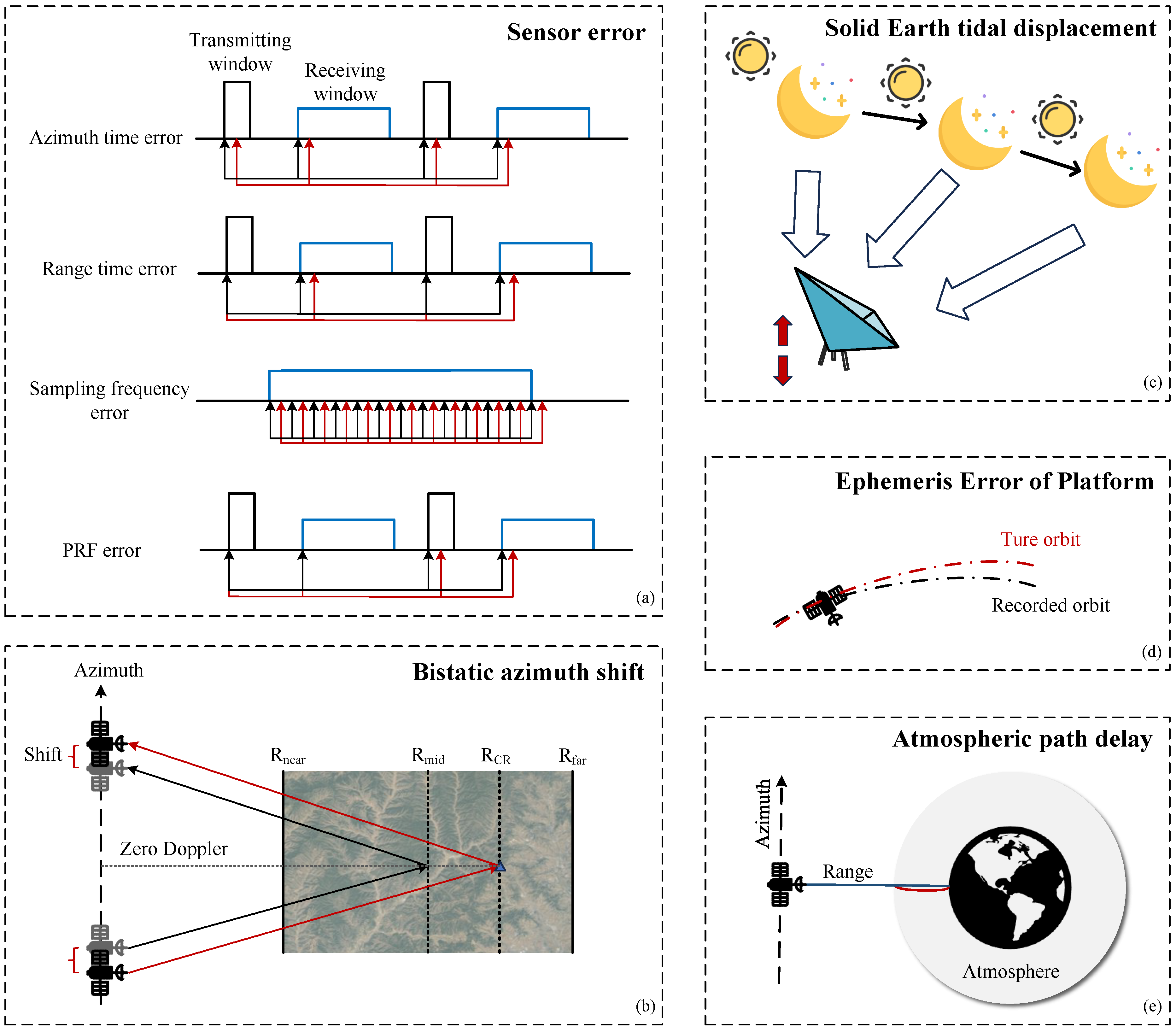
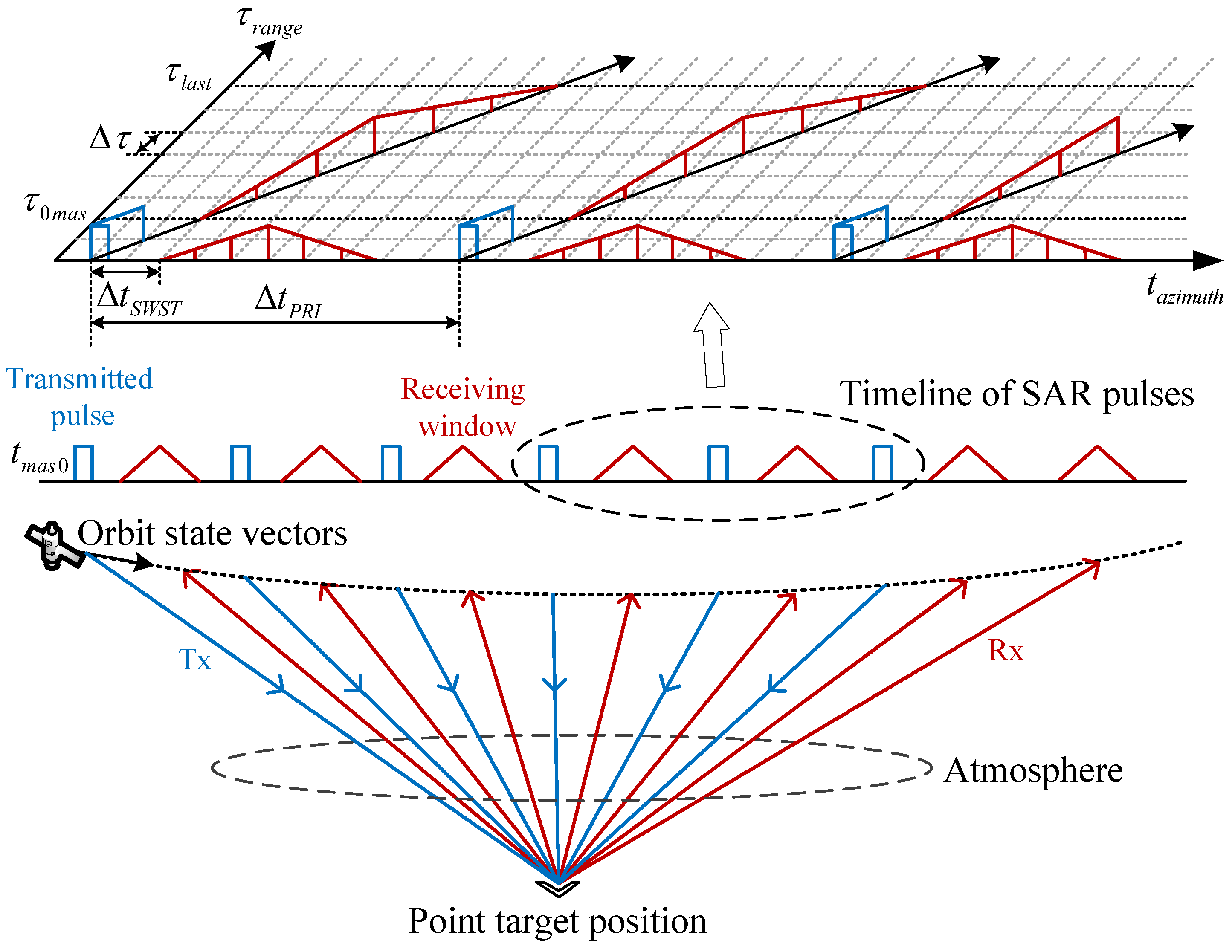
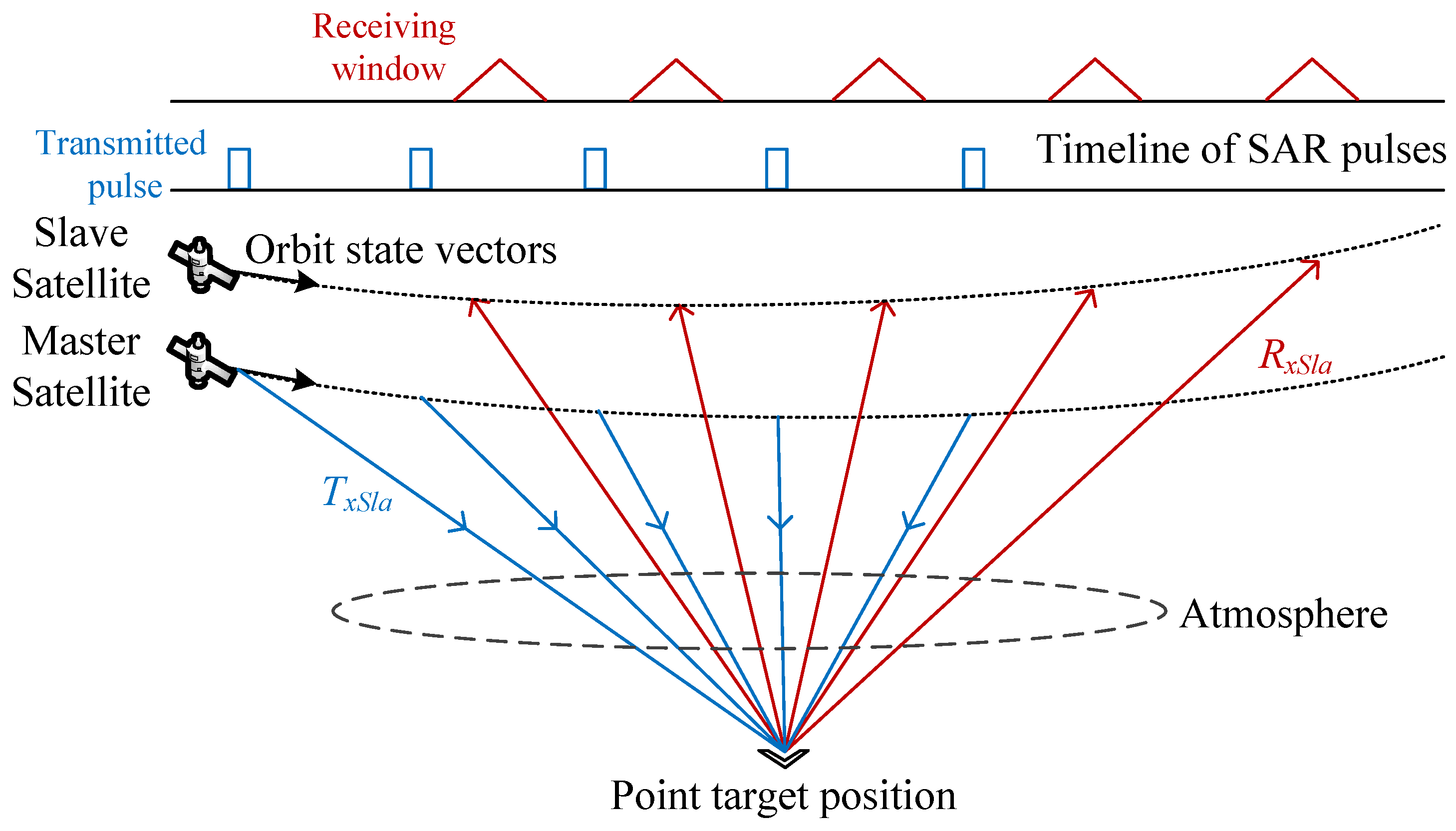
2.1. Geometric Distortions

Before establishing the geometric calibration model, we analyze the sources of geometric distortions in the uncorrected data. These sources mainly include sensor error, bistatic azimuth shift, solid Earth tidal displacement, ephemeris error of platform, and atmospheric path delay [2,5,6,7,8].
1.
Sensor error.
Sensor error can result in four types of systematic time errors, namely: azimuth time error, range time error, sampling frequency error, and pulse repetition frequency (PRF) error [32]. As shown in Figure 1a, the recorded time by the system is indicated by the black arrow, but sensor errors cause time inaccuracies, as shown by the red arrow.
  • Azimuth time error.
Azimuth time error is caused by the timing error of the time control unit in the system equipment. The time control unit records the system time of all events with a specific timing accuracy and record frequency. Due to the low updating frequency of the time control unit, which does not match the pulse frequency of the SAR, all recorded times are displaced. The direct manifestation of this error is the initial azimuth time error in the auxiliary data.
  • Range time error.
The phenomenon of radar signals traversing the signal channel’s components causes systematic delay errors. These errors generate discrepancies in the recorded time stamps for the beginning of echo pulse reception. Consequently, temporal offset appears as the initial range time error in the auxiliary data.
  • Sampling frequency error.
Sampling frequency error results from the nominal value error of the system oscillator and the stability of the crystal oscillator, leading to a deviation between the real sampling frequency of the SAR system and the sampling frequency used for imaging and location processing.
  • PRF error.
The long-term drift of the local oscillator causes variations in the PRF, which affects the pixel spacing in the azimuth direction due to the conversion of the fractional error of the local oscillator frequency into a corresponding decimal part error of the PRF, resulting in a proportional error in the azimuth direction.
The sampling frequency and PRF inaccuracies are primarily caused by the crystal oscillator’s inherent stability. Long-term stability and short-term stability of the crystal oscillator in LT-1 are on the order of 10 7 and 10 10 , indicating high precision. As a result, the sampling frequency and PRF errors caused by this oscillator’s stability are so minute that they can be disregarded.
2.
Bistatic azimuth shift.
Bistatic azimuth shift is equivalent to start-stop approximation, which postulates that the SAR remains stationary during the transmission and reception of the same pulse. However, within the same azimuth, different ranges correspond to distinct transmission and reception positions [7]. Consequently, the satellite’s movement during the pulse transmission, reception, and duration of pulse reception leads to azimuthal errors that vary with ranges. In the subsequent development of the geometric calibration model, we are concerned with the continuous motion of the actual satellite movement. This choice effectively averts the emergence of such errors.
3.
Solid Earth tidal displacement.
Tidal displacement of Earth’s crust is induced by the gravitational forces of the Sun and Moon [8]. It can be computed using the conventional geodynamic model, which is aligned with established geodetic reference frames. This computation results in temporal corrections for both range and azimuth measurements. The consequential impact varies between 0.2 m in the range direction and 0.05 m in the azimuth direction  [33]. These variations are contingent on the specific geographic location and the relative positions of the Sun and Moon. Given the relatively minor magnitude of the effect of this particular error, it will not be considered within the scope of this study.
4.
Ephemeris error of platform.
The ephemeris error of the platform includes both position and velocity errors [2]. Positional inaccuracies of the platform can potentially introduce errors in the azimuth and range directions. However, orbit parameters comprise data that have been meticulously processed, resulting in extremely accurate results. The accuracy of precise orbit data can approach the decimeter or centimeter scale. After meticulous processing, the platform’s ephemeris error can be interpreted as exhibiting random characteristics.
5.
Atmospheric path delay.
Atmospheric path delay refers to the additional delay error caused by atmospheric effects during signal propagation, which impacts the range direction. Tropospheric delay and ionospheric delay are the origins of atmospheric path delay. The tropospheric influence can exhibit variations ranging from 0.5 m to 4.5 m depending on atmospheric conditions and geographic location. Similarly, the ionospheric impact can vary between 1 m and 20 m based on geographic location and solar activity  [33].
The atmospheric path delay is an error influenced by external environmental factors that vary with atmospheric properties and are not subject to systematic biases [34]. Nevertheless, it can still introduce errors in range time measurements and can not be neglected. Consequently, it necessitates elimination in the calibration process.
In summary, the geometric calibration in this paper aims to rectify inherent biases within the SAR system, particularly correcting range and azimuth time errors caused by sensor errors. Additional error factors considered in this study include bistatic azimuth shift and atmospheric path delay. In contrast, solid Earth tidal displacement and ephemeris error of the platform are not addressed within the scope of this paper. To achieve precise geometric geolocation, LT-1’s range time error accuracy must be greater than 5 ns, and its azimuth time accuracy must be greater than 0.1 ms. This guarantees that both range and azimuth geolocation are accurate to within 0.8 m.

2.2. Geometric Calibration Model of Master SAR

The observation scheme of the master SAR is depicted in Figure 2. In bistatic mode, the master SAR transmits the signal pulses at time t T x and receives the backscatter signal from the point target at time t R x , and it can be considered equivalent to a monostatic SAR.
According to Figure 2, the receiving time associated with the pixel coordinates of the point target on the master SAR image is:
t R x ( m m a s , n m a s ) = t m a s 0 + t m a s 0 e r r + m m a s Δ t P R I + Δ t S W S T + n m a s Δ τ
where m m a s is the azimuth pixel coordinate of the point target on the master SAR image, n m a s is the range pixel coordinate of the point target on the master SAR image, t m a s 0 represents the measured value of the initial azimuth time, t m a s 0 e r r is the systematic error of the initial azimuth time, Δ t P R I represents the azimuth pulse repetition interval, Δ t S W S T represents the sampling window start time, and Δ τ represents the range sampling time interval.
Additionally, the two-way pulse round trip time τ n m a s can be expressed as:
τ n m a s = τ m a s 0 + τ m a s 0 e r r + n m a s Δ τ + R a t c
where τ m a s 0 is the measured value of the initial range time, τ m a s 0 e r r is the systematic error of the initial range time, R a t is the atmospheric path delay. The corresponding slant range from satellite to ground point target is:
R m a s = c τ n m a s 2 = c 2 τ m a s 0 + τ m a s 0 e r r + n m a s Δ τ + R a t c
where R m a s is the slant range, and c is the speed of light.
According to the signal transmission path shown in Figure 2, the transmitting time is:
t T x ( m m a s , n m a s ) = t R x ( m m a s , n m a s ) τ n m a s
The imaging time for the focused SAR image is in the middle between the transmitting time and the receiving time:
t m a s ( m m a s , n m a s ) = 1 2 t R x ( m m a s , n m a s ) + t T x ( m m a s , n m a s )
Then, we can obtain the RD equation of the master SAR:
R m a s = P M t m a s P G C P f d M = 2 P M t m a s P G C P V M t m a s λ P G C P P M t m a s
where P G C P = X G C P , Y G C P , Z G C P T represents the coordinate of the point target, superscript T indicates matrix transpose, V M denotes the velocity of the master SAR, f d M represents the Doppler centroid frequency of the master SAR, and P M = X M , Y M , Z M T is the coordinate of the master SAR. Notably, all coordinates mentioned in this paper are defined within the Earth-centered, Earth-fixed (ECEF) coordinate system. The ECEF coordinate system is a three-dimensional Cartesian coordinate system with its origin at the center of the Earth and its axes aligned with the Earth’s rotation.
Given the low sampling frequency of the global navigation satellite system (GNSS), acquiring the position corresponding to each azimuth sampling time is necessary through up-sampling. In this study, we use polynomial functions, specifically Equation (7), to model the satellite orbits’ state vector.
P M t = X M t Y M t Z M t = k = 0 N k a M k t k k = 0 N k b M k t k k = 0 N k c M k t k
where N k is the polynomial degree, and N k is set to 3 in this paper; a M k , b M k , and c M k are the polynomial coefficients; t is the time and is the independent variable of the polynomial function. We use the least squares method to fit the polynomial coefficients of the polynomial function by the available data recorded by GNSS. This approach permits an accurate estimation of the satellite’s position at any given time within the azimuth sampling interval.
To maintain consistency between position and velocity, the satellite’s velocity can be derived by taking the derivative of the position polynomial concerning time, and the satellite’s velocity can be expressed as:
V M t = V X M t V Y M t V Z M t = k = 0 N k 1 k a M k t k 1 k = 0 N k 1 k b M k t k 1 k = 0 N k 1 k c M k t k 1
Take P m a s = t m a s 0 e r r , τ m a s 0 e r r T as the geometric calibration parameter of the master SAR and bring it into the RD equation to obtain the calibration equation:
F 1 ( P m a s ) = P M t m a s P G C P c τ n m a s 2 = 0 F 2 ( P m a s ) = 2 V M t m a s P M t m a s P G C P λ P M t m a s P G C P f d M = 0

2.3. Geometric Calibration Model of Slave SAR

The observation geometry of the slave SAR is depicted in Figure 3. t T x S l a can be considered the transmitting time of the master SAR, and its corresponding transmitting slant range is T x S l a . In addition, t R x S l a can be considered the receiving time of the slave SAR, leading to the receiving slant range of R x S l a . Similarly to the master SAR, the receiving time associated with the pixel coordinate of the point target on the slave SAR image is:
t R x S l a ( m s l a , n s l a ) = t s l a 0 + t s l a 0 e r r + m s l a Δ t P R I + Δ t S W S T + n s l a Δ τ
where m s l a is the azimuth pixel coordinate of the point target on the slave SAR image, n s l a the range pixel coordinate of the point target on the slave SAR image, t s l a 0 is the measured value of the initial azimuth time of the slave SAR, and t s l a 0 e r r is the systematic error of the initial azimuth time. Due to the same internal clock settings of the main and slave SAR, the slave SAR has the same Δ t PRI , Δ t SWST , and Δ τ as the master SAR.
The two-way pulse round trip time of the slave SAR τ n s l a can be expressed as:
τ n s l a = τ s l a 0 + τ s l a 0 e r r + n s l a Δ τ + R a t c
where τ s l a 0 is the measured value of the initial range time of the slave SAR, and τ s l a 0 e r r is the systematic error of the initial range time. According to the signal transmission path, the transmitting time is:
t T x S l a ( m s l a , n s l a ) = t R x S l a τ n s l a
The two-way slant range of the pulse trip is:
R s l a = T x S l a + R x S l a = c τ n s l a
The RD model of the slave SAR is:
T x S l a = P M t T x S l a P G C P R x S l a = P S t R x S l a P G C P f d S = V M t T x S l a P M t T x S l a P G C P λ P M t T x S l a P G C P + V S t T x S l a P S R x S l a P G C P λ P S t R x S l a P G C P
where P M t T x S l a = X M t T x S l a , Y M t T x S l a , Z M t T x S l a T is the trajectory coordinate of the master SAR at transmitting time, which is acquired by taking t T x S l a into Equation (7); V M = V X M t T x S l a , V Y M t T x S l a , V Z M t T x S l a T is the corresponding velocity vector of the master SAR at transmitting time; f d S is the Doppler centroid frequency; P S t R x S l a and V S t R x S l a are trajectory coordinates and velocity vector of the slave SAR at the receiving time, respectively. Similarly to the master SAR, the approach for fitting the trajectory of the slave SAR is as follows:
P S t = X S t Y S t Z S t = k = 0 N k a S k t k k = 0 N k b S k t k k = 0 N k c S k t k , V S t = V X S t V Y S t V Z S t = k = 0 N k 1 k a S k t k 1 k = 0 N k 1 k b S k t k 1 k = 0 N k 1 k c S k t k 1
where a S k , b S k , and c S k are the polynomial coefficients.
The systematic time errors of the slave SAR are set as the calibration parameters P s l a = t s l a 0 e r r , τ s l a 0 e r r T . The geometric calibration model is established as Equation (16) by Equations (10), (12)–(14).
F 3 ( P ) = P M t T x S l a P G C P + P S t R x S l a P G C P c τ n s l a = 0 F 4 ( P ) = V M t T x S l a P M t T x S l a P G C P λ P M t T x S l a P G C P + V S t R x S l a P S t R x S l a P G C P λ P S t R x S l a P G C P f d S = 0
Therefore, the calibration parameters can be obtained by solving Equation (16).

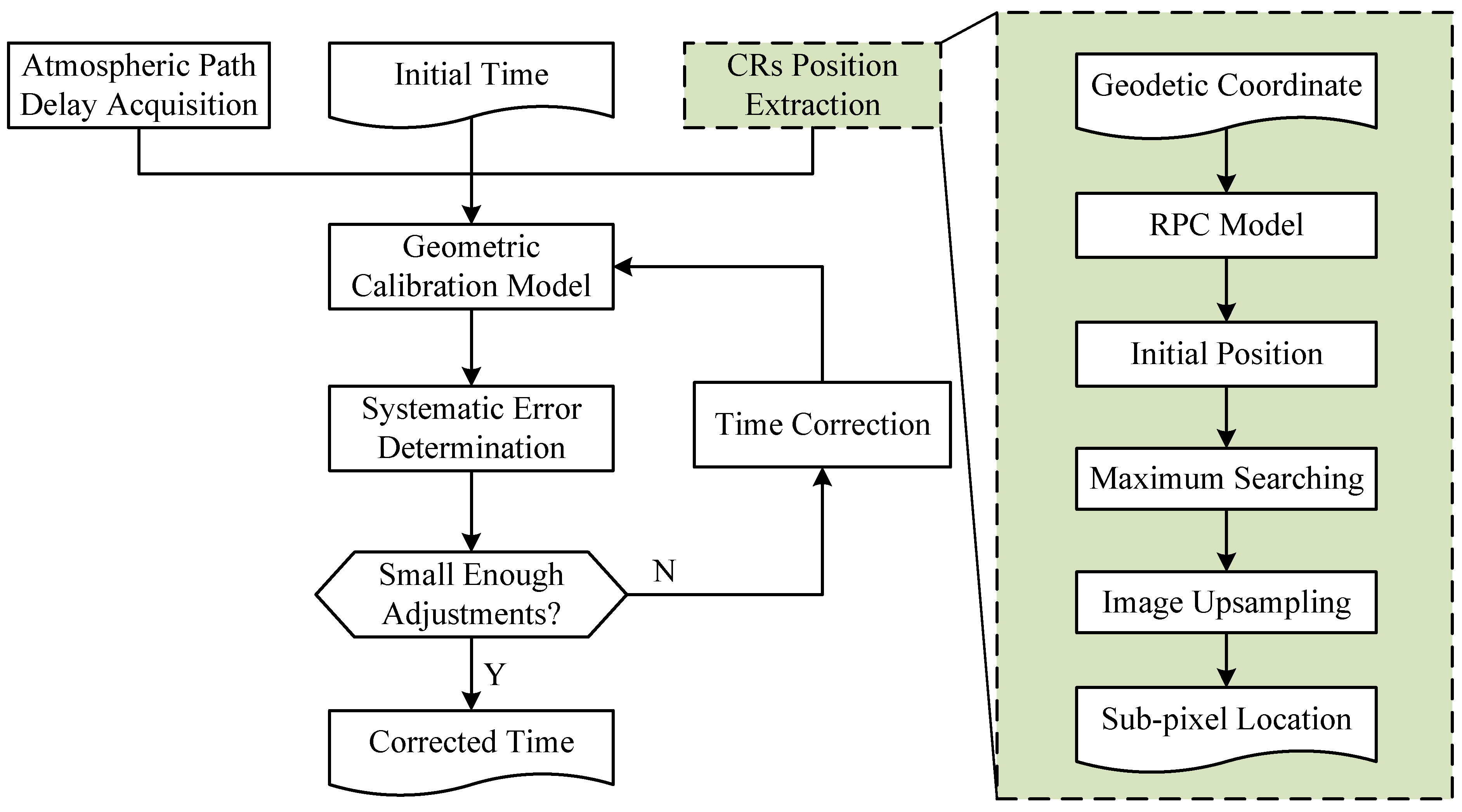
2.4. Atmospheric Path Delay Correction

In this section, the focus is on addressing the influence of atmospheric conditions on SAR measurements. The atmospheric path delay is composed of ionospheric delay and tropospheric delay.
Tropospheric delay can be derived from the ERA5 reanalysis product released by the European Centre for Medium-Range Weather Forecasts (ECMWF) [2]. In addition, the tropospheric delay can also be obtained by the Generic Atmospheric Correction Online Service for InSAR (GACOS) model [35,36,37]. The tropospheric delay can be calculated using the following equations [38]:
L t r o = 10 6 h 0 N d h = 10 6 i n 1 N i + N i + 1 × h i + 1 h i / 2
N = k 1 ( P e ) T + k 2 e T + k 3 e T
e = q × P 0.622 + 0.378 q
where L t r o is the tropospheric delay, h 0 represents the surface height, N is the atmospheric refractive index, n is the total number of pressure levels contained within the ERA5 data above the station, h i refers to the height of i-th level, P denotes the surface pressure (in hPa), e signifies the surface water vapor pressure (in hPa), T is the surface temperature (in K), q is specific humidity, and k 1 , k 2 , and k 3 are constants equal to 77.604 K/hPa, 64.79 K/hPa, and 377,600 K 2 / hPa, respectively.
Additionally, the ionospheric delay can be calculated by [39]:
L i o n = 40.28 × T E C f 2
where L i o n is the ionospheric delay, T E C is the total electron content data provided by the Center for Orbit Determination in Europe (CODE), and f is the frequency of the radar signal.
Therefore, the radar signal transmission delay error caused by the atmospheric influence in the slant range direction is:
R a t = L t r o + L i n o cos φ
where φ is the incidence angle.

2.5. Model Resolving

In previous sections, we have developed the geometric calibration model for the master and slave SARs, requiring the determination of precise calibration parameters. However, due to the inherent complexity of the equation, obtaining a closed-form expression for these parameters poses a considerable challenge. To facilitate the solution process, we propose to employ the Taylor expansion to expand the calibration equation systematically. By utilizing this approach, we aim to derive an approximate solution that will aid in effectively addressing the complexities associated with solving the calibration parameters.
Firstly, solve the geometric calibration model of the master SAR. Denote the calibration equation by F, the calibration parameter by P m a s , and the initial value of the calibration parameter by P m a s 0 . The Taylor expansion of F at P m a s 0 is:
F P m a s = F P m a s P m a s = P m a s 0 p + F ( P m a s 0 ) = 0
where p = P m a s P m a s 0 .
Given the simultaneous determination of two calibration parameters (initial range time and initial azimuth time), the two calibration equations must be solved concurrently. Equation (22) is therefore expressed in matrix form as follows:
A p + F ( P m a s 0 ) = 0
where
F ( P m a s 0 ) = [ F 1 ( P m a s 0 ) , F 2 ( P m a s 0 ) ] T
A = F 1 P m a s t m a s 0 e r r P m a s = P m a s 0 F 1 P m a s τ m a s 0 e r r P m a s = P m a s 0 F 2 P m a s t m a s 0 e r r P m a s = P m a s 0 F 2 P m a s τ m a s 0 e r r P m a s = P m a s 0
The solution of Equation (23) can be acquired by minimizing the 2-norm of residuals:
p ^ = arg min A p + F ( P m a s 0 ) 2
The best-unbiased estimation of the calibration parameter is:
p ^ = A T A A T E
where E is the error matrix and E = F ( P m a s 0 ) , and superscript † indicates pseudo-inverse.
Thus, the estimation of P m a s is:
P ^ m a s = P m a s 0 + p ^ .
The preceding analysis reveals that improved accuracy in estimating the systematic time error corresponds to continuously reduced errors in range and Doppler. Consequently, an iterative process is necessary to enhance the precision of systematic time error estimation. In this study, the termination criteria for the iterative procedure are set as p ^ < 10 10 , leading to a final iteration that adjusts the time error to a value smaller than 10 10 s.
Regarding the geometric calibration model for the slave SAR, the solution method is comparable to the one used for the master SAR, as was previously discussed. Nonetheless, the matrix A for the slave SAR has distinct expressions, as shown below:
A = F 3 P s l a t s l a 0 e r r P s l a = P s l a 0 F 3 P s l a τ s l a 0 e r r P s l a = P s l a 0 F 4 P s l a t s l a 0 e r r P s l a = P s l a 0 F 4 P s l a τ s l a 0 e r r P s l a = P s l a 0
where F 3 and F 4 are the geometric calibration equations of the slave SAR found in Equation (16), P s l a is the calibration parameter of the slave SAR, and P s l a 0 is the initial value of the calibration parameter.
The flowchart illustrating the geometric calibration process is depicted in Figure 4. The atmospheric path delay is initially estimated based on the principles elucidated in Section 2.4.
Subsequently, the positions of CRs on the image are obtained. The derivations in Section 2 underscore the significance of accurate geolocation of calibration points on the image, as it constitutes a critical input parameter determining the upper limit of geometric calibration accuracy. We employ the procedure described within the green box in Figure 4 for position searching to achieve efficient and precise automatic detection of calibration targets in SAR images, thereby preventing manual searching.
As shown in the green box in Figure 4, the geodetic coordinates of the CRs are input into the rational polynomial coefficients (RPC) model to derive the initial coordinates of the CRs on the SAR image. The RPC model is a mathematical model utilized for geometric correction and geolocation of remote sensing images [40,41]. Rational polynomials are employed in the RPC model to approximate the mapping relationship between image pixel coordinates and geographical coordinates. The Level 1 imaging products of LT-1 provide RPC files that can be directly utilized for this purpose. However, inherent geolocation errors persist since the RPC model does not incorporate geometric correction. Consequently, it becomes necessary to establish a 50 × 50 search window centered at the initial coordinates and search for the maximum image amplitude, serving as the actual position of the CRs.
Moreover, the image is upsampled in the frequency domain to yield the image coordinates of the CRs at the sub-pixel level. Upon inputting the Single Look Complex (SLC) image and the geodetic coordinates of CRs, the plugin can calculate the sub-pixel level positions of CRs on the SAR image within 1 s. This approach effectively eliminates the necessity for manual calibration of point searching, leading to significant time and effort savings.
Subsequently, the initial range time and initial azimuth time parameters are read from the auxiliary files of the SAR image as input, and Algorithm 1 is utilized to calculate the systematic time errors.
Algorithm 1 Calibration parameter derivation.
Input: SLC images and their auxiliary files, coordinates of CRs, and atmospheric delay.
Initialization: Set the initial values of the calibration parameters P 0 as (0,0) and F l a g = 1 . Repeat the following steps until F l a g is smaller than 10 10 :
     Step 1: Compute the Jacobian matrix A using Equations (25) and (29).
     Step 2: Calculate the error matrix E using F ( P 0 ) based on Equations (6) and (14).
     Step 3: Compute the best unbiased estimation of p using A T A A T E .
     Step 4: Calculate the best estimation of P as P ^ = P 0 + p ^ .
     Step 5: Update the initial values of the calibration parameters P 0 to P ^ .
     Step 6: Update the value of F l a g with p ^ .
Output: Calibration parameter P .

3. Results and Analysis

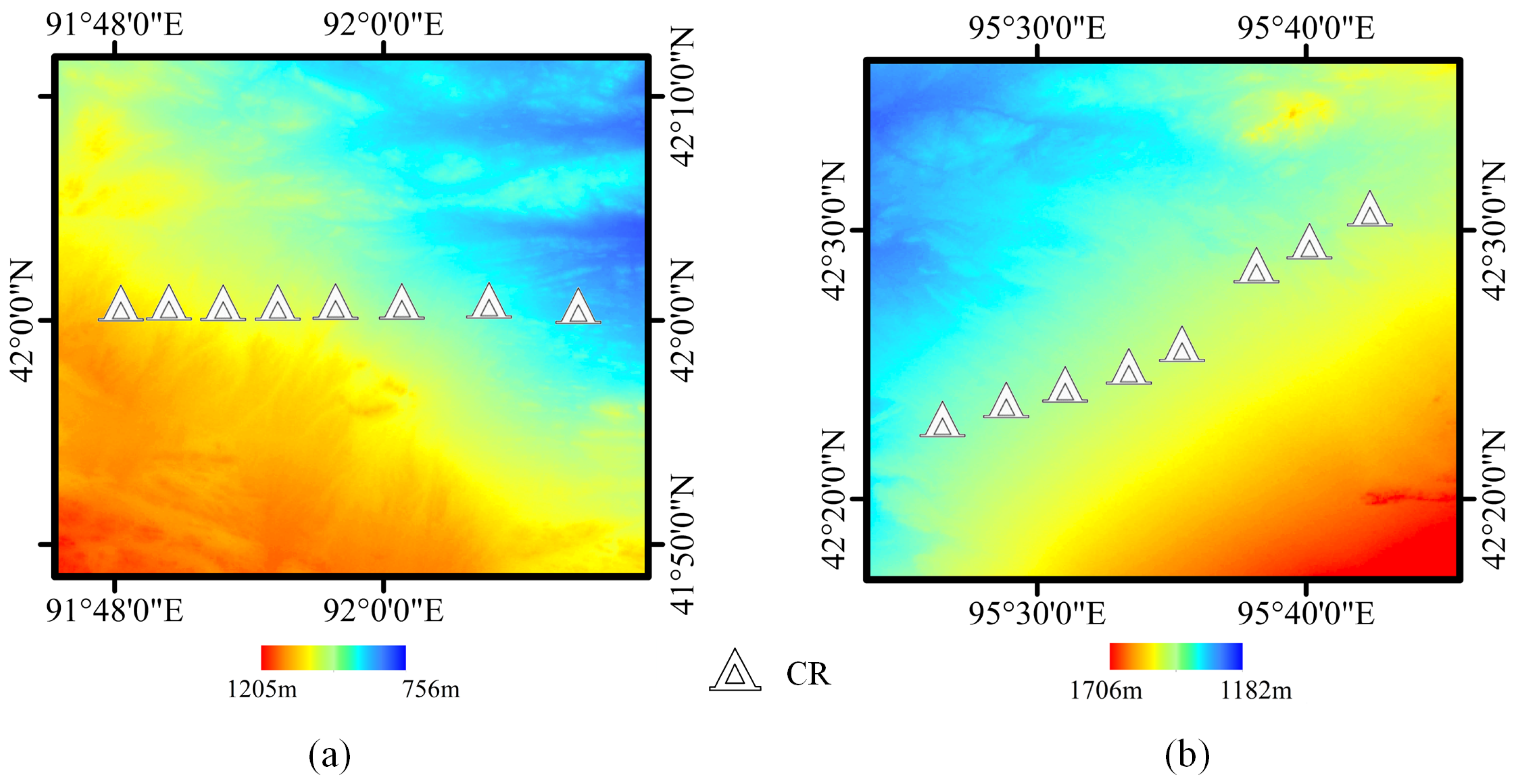
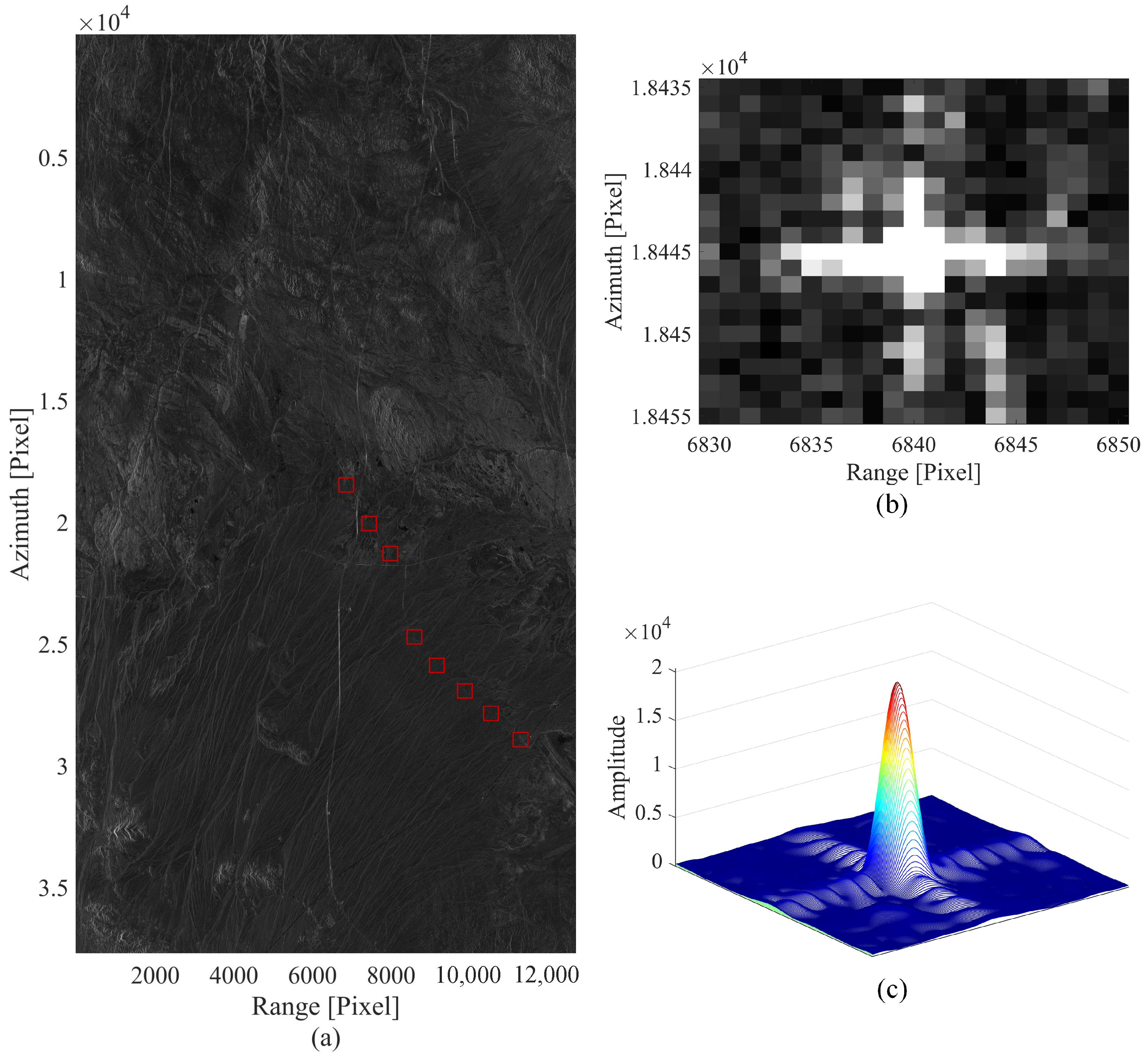
3.1. Study Area and Datasets

Two distinct sites in Xinjiang, China, were judiciously selected to accomplish geometric calibration, and CRs were strategically installed at these coordinates based on the satellite track map. The topographic delineation of these selected sites is visually conveyed in Figure 5, where white triangles accurately mark the geolocation of the CRs. These specifically chosen areas, hallmarked by their arid environmental conditions, minimal vegetation cover, and uniform backscattering coefficients, are optimally conducive for serving as calibration sites.
The incidence angle range of LT-1 is specified to be between 20° and 46° [42]. Analyzing the trajectory of LT-1 reveals that it will illuminate test site A with an incidence angle exceeding 40° and test site B with an incidence angle of approximately 20°. As a result, test site A represents the far-range beam site, while test site B represents the near-range beam site. This design ensures avoidance of the beam dependency hypothesis observed in Sentinel-1 [16], where distinct azimuth time and range time errors are associated with different beams.
In June, the LT-1 satellite formation attained a stable orbit. The deployment of CRs and the measurement of their three-dimensional positions were completed by the beginning of July. After meticulous planning for satellite imaging, LT-1 successfully observed the CRs on 7 July, producing high-quality SAR images with excellent focus. We chose 30 bistatic images acquired by the LT-1 from July to November 2022. Table 1 lists the specific dates and their corresponding scene numbers. These images were captured using HH polarisation and strip mode. Note that each scene number corresponds to two images acquired in bistatic mode by LT-1A and LT-1B.
To comprehensively elucidate the entirety of LT-1’s geometric calibration process, we randomly selected two pairs of SAR images acquired by LT-1 on 8 September 2022. The specific parameters of the data are presented in Table 2.

3.2. Geometric Calibration of Example Data

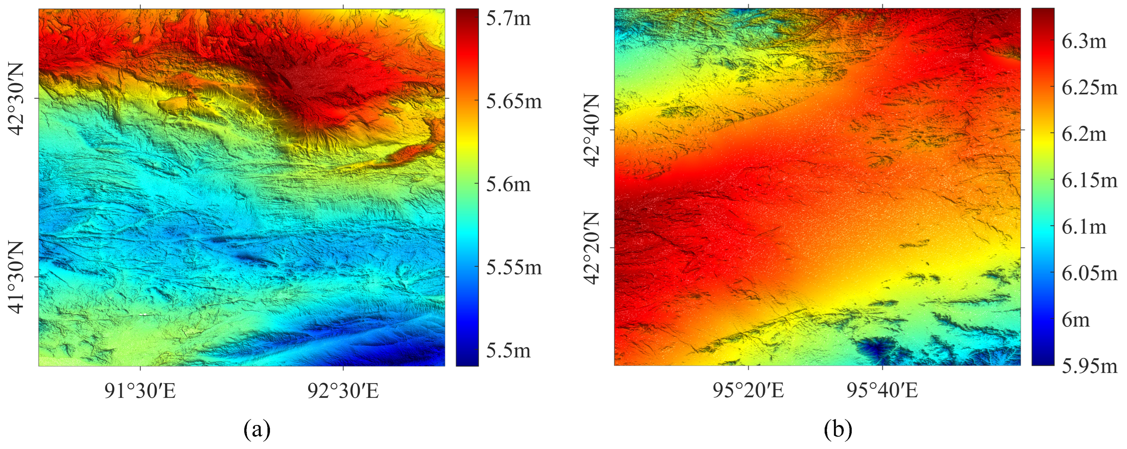
3.2.1. Atmospheric Path Delay Acquisition

In this section, we focus on estimating atmospheric path delay. We employed the Shuttle Radar Topography Mission (SRTM) DEM and the high-resolution ECMWF weather model at 0.1° and 6-h resolutions to calculate the tropospheric delay for test sites A and B. The values of tropospheric delay fall within the range of 1.851 m to 2.364 m at these two sites.
Based on the CODE ionospheric TEC dataset with a latitude and longitude resolution of 5° × 2.5° and a temporal resolution of 1 h, the ionospheric delays at two experimental locations were determined to be 3.5532 m and 4.235 m, respectively. Figure 6 illustrates the total atmospheric path delay at test sites A and B for an incident angle of 0°.
To obtain the total atmospheric delay error generated by SAR propagation to the CRs, matching the geodetic coordinates of the CRs with Figure 6 is required. For the case of vertical incidence, the mean atmospheric path delay at the CRs in test site A is determined to be 5.516 m, while in test site B, it is found to be 6.392 m.
It is important to highlight the role of radar incident angles in SAR signal propagation, as higher incident angles result in increased atmospheric path delay. Therefore, we consider the weighted impact of radar incident angles. Specifically, at test site A, the incident angle is 44.365°, while at test site B, it is 22.440°. Consequently, the average atmospheric path delay computed for the radar signal at test site A is 7.715 m, whereas at test site B, it amounts to 6.9157 m.

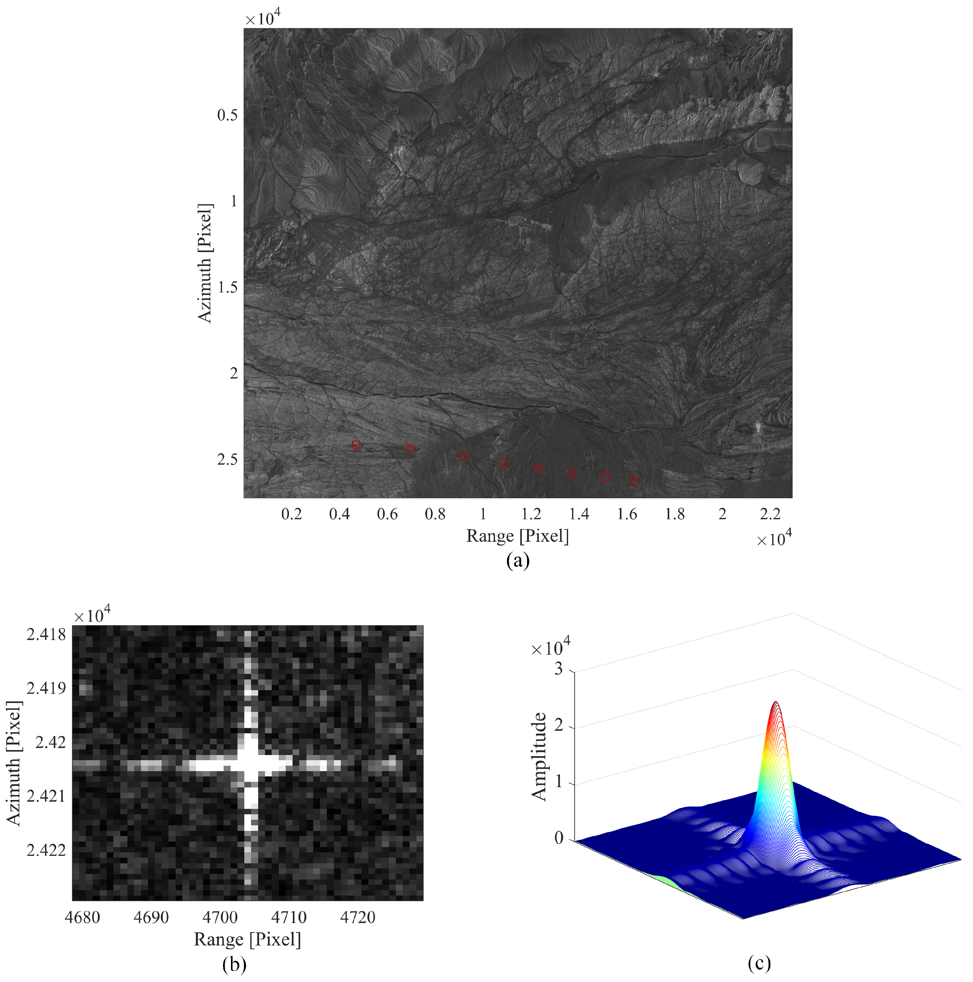
3.2.2. CRs Position Extraction

We employ localization techniques utilizing the RPC data, maximum amplitude value search, and upsampling image operations as mentioned in Section 2.5 to accurately determine CRs’ positions on the image.
To visually depict the localization results of test site A, we present the positions of CRs on the magnitude image of the SLC data for test site A in Figure 7a. The red boxes in the figure indicate the positions of the CRs on the image, corresponding to the eight targets listed in Figure 5a. Additionally, we magnified the image of the first CR in Figure 7b. The shape of the CR can be seen clearly in the illustration, indicating that the CR has been successfully localized.
After successfully determining the initial positions of the CRs, the subsequent step involves an upsampling procedure, where the peak amplitude value obtained from Figure 7b serves as the central reference. The resulting upsampled amplitude map is visually depicted in Figure 7c. The precise sub-pixel position of the initial CR is determined by identifying the peak’s coordinates within Figure 7c. It is worth noting that the CR exhibits an intensity of 28,000, which significantly surpasses the average magnitude of adjacent signals by a factor of no less than 300. This indicates an exceptionally robust echo power and a signal-to-noise ratio (SNR) exceeding 25 dB. The minimal geolocation precision, or standard deviation (STD), is theoretically linked to the SNR and resolutions [43]. Leveraging the SNR and resolutions of the selected data, the theoretical geolocation precision in the azimuth and range directions is calculated to be 0.046 m and 0.038 m, respectively. This outstanding performance undeniably establishes the CR we deployed as a precious instrument for calibration purposes.
Similarly, the results related to the localization of the CRs at test site B are depicted in Figure 8. Figure 8a illustrates the coordinates of the calibration point corresponding to Figure 5b, while Figure 8b presents an enlarged view of the first CR. Furthermore, Figure 8c showcases the upsampled amplitude map obtained through the aforementioned process. The peak intensity in Figure 8c is measured at 20,000, yielding an associated SNR of 23.01 dB. The theoretical geolocation precision is computed for both azimuth and range directions, resulting in values of 0.048 m and 0.045 m, respectively.
We observe that the shape of the CR image at test site B in Figure 8b appears less prominent than the results obtained at test site A in Figure 7b. This distinction can be attributed to the consistent slant range sampling intervals between the two sites, while the incident angle at test site B is smaller than at test site A, resulting in the ground range sampling interval at test site B being correspondingly reduced. Specifically, the incident angle at test site A was measured at 44.496°, whereas at test site B, it was recorded as 22.440°. As a result, the ground range sampling interval at test site A is twice that of test site B. Consequently, the angular shape of the corner reflector in Figure 7b exhibited a more pronounced appearance than the shape observed in Figure 8b.
Furthermore, due to the significant overlap between the master and slave SAR images, the localization results of the slave SAR closely resemble those of the master SAR. In this context, we focus our presentation on the SLC image and localization results of the master SAR.
Accurate localization of the CRs on SAR images establishes a fundamental basis for subsequent procedures, facilitating precise geometric calibration and accurate interpretation of SAR data.

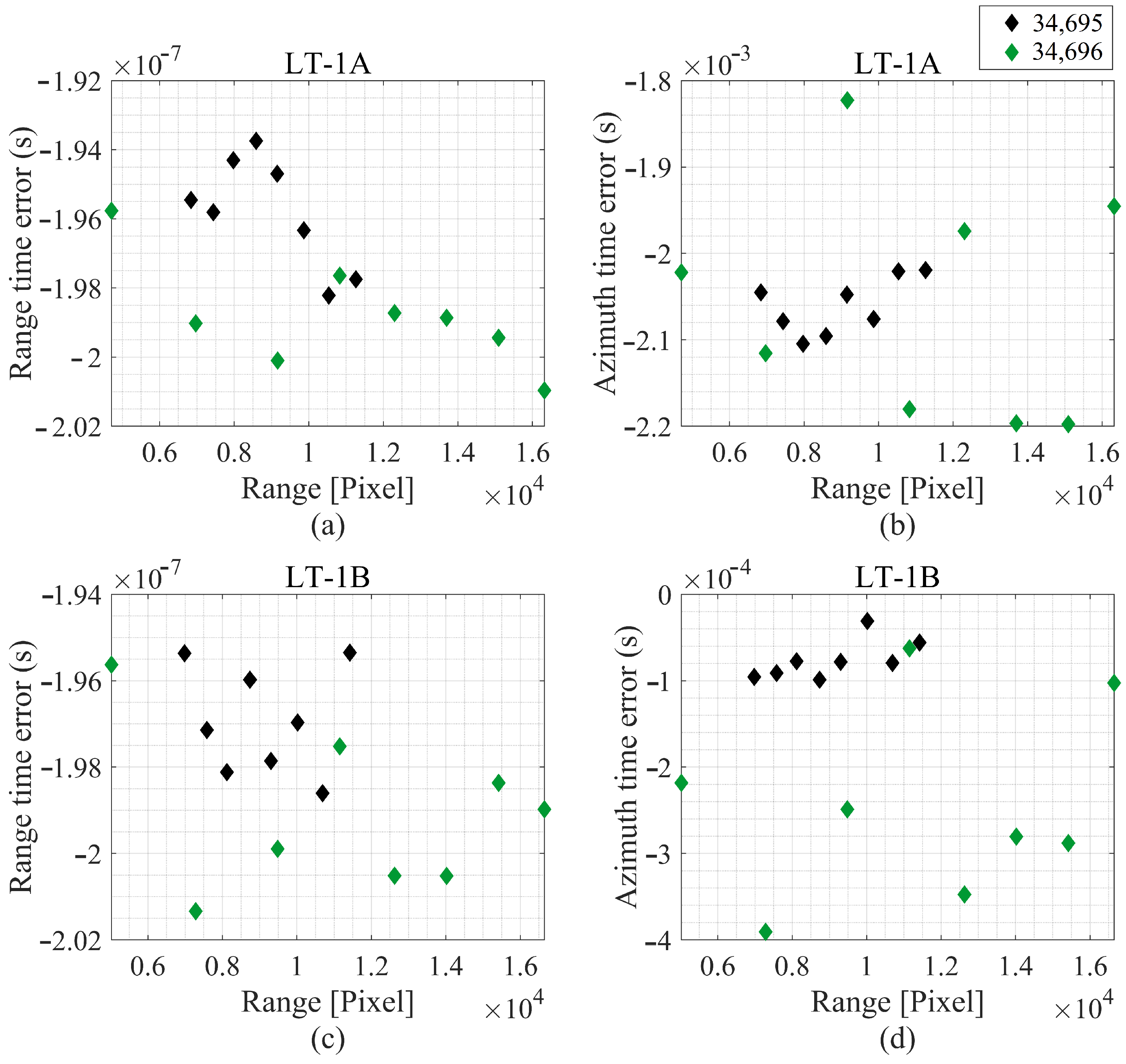
3.2.3. Systematic Error Determination

We can proceed with geometric calibration based on the proposed Algorithm 1 from Section 2.5. The outcomes are presented in Figure 9, where Figure 9a,b illustrate the range and azimuth time error results for LT-1A, respectively. Figure 9c,d portray the range and azimuth time error results for LT-1B, respectively. The green markers denote the results for test site A, while the black markers represent the outcomes for test site B. The statistical results are shown in Table 3.
From Figure 9 and Table 3, we observe that the results obtained under two different beams are consistent, which helps us rule out the beam dependency hypothesis. Combining the results from the two test sites, we find that the average range time error for LT-1A is 197.610 ns, and the average azimuth time error is 2.058 ms. As for LT-1B, the average range time error is 198.010 ns, and the average azimuth time error is 0.159 ms. The STD of the range time error for LT-1A and LT-1B are 2.161 ns and 1.975 ns, respectively, satisfying the precision requirement of 5 ns. The STD of the azimuth time error for LT-1A and LT-1B are 0.096 ms and 0.085 ms, meeting the precision requirement of 0.1 ms.
Furthermore, we note a consistent result in the range time error for LT-1A and LT-1B, with a discrepancy of only 0.4 ns between them. This minor difference can be attributed to the residual error caused by range time synchronization, which is a commendable performance in LT-1 [24].
Subsequently, we computed the absolute location errors (ALE) caused by systematic time errors, as presented in Table 3. For LT-1A, systematic time errors led to a range geolocation error of 29.621 m and an azimuth geolocation error of −15.726 m, resulting in an overall geolocation error of 33.537 m. Similarly, for LT-1B, the existence of the system time error caused a range geolocation error of 29.681 m and an azimuth geolocation error of −1.208 m, culminating in an overall geolocation error of 29.706 m. These errors can be effectively eliminated after geometric calibration.

3.3. Long-Term Monitoring of Geometric Calibration

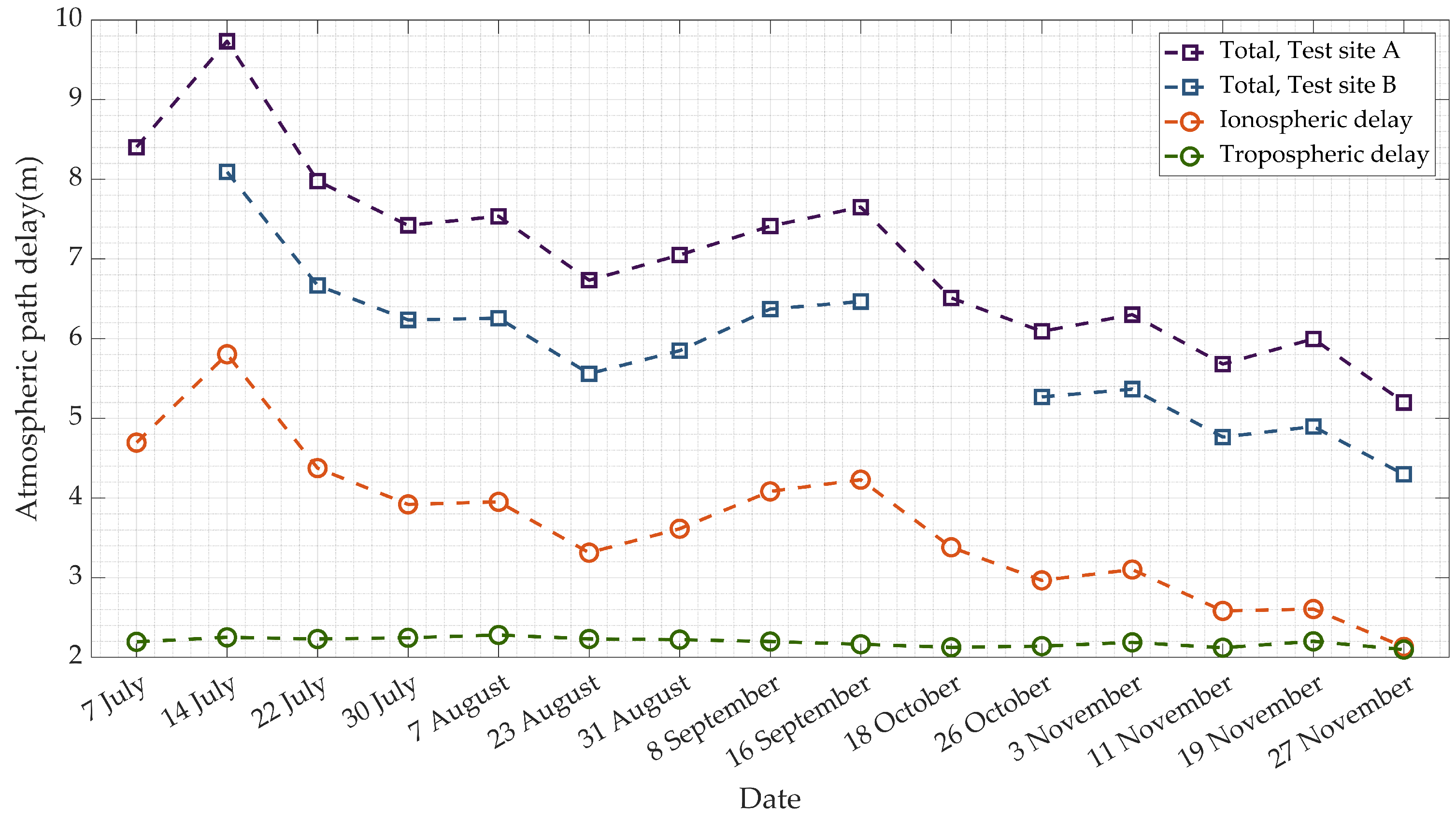
3.3.1. Atmospheric Path Delay Acquisition

Section 3.2 introduced the overall geometric calibration process using sample data. This section aims to present statistical results for the geometric calibration of all scenes from July to November based on the same process in Section 3.2. As shown in Figure 10, we first analyze the atmospheric path delay.
Atmospheric path delay results on 7 July and 18 October are missing for test site B because the CRs are outside the image extent in these scenes. The orange and green markers in Figure 10 represent vertical ionospheric delay and tropospheric delay, respectively. Figure 10 shows that the tropospheric delay is highly stable at 2.194 m, and the ionospheric delay exhibits a trend toward decreasing values.
We weigh the atmospheric delays based on the SAR electromagnetic wave incidence angles for sites A and B. The total atmospheric delay for test site A decreases from 9.732 m to 5.201 m, as shown by the purple marker in Figure 10, while it decreases from 8.094 m to 4.297 m for test site B, as indicated by the blue marker in Figure 10. The calibration model can then make adjustments based on these values.

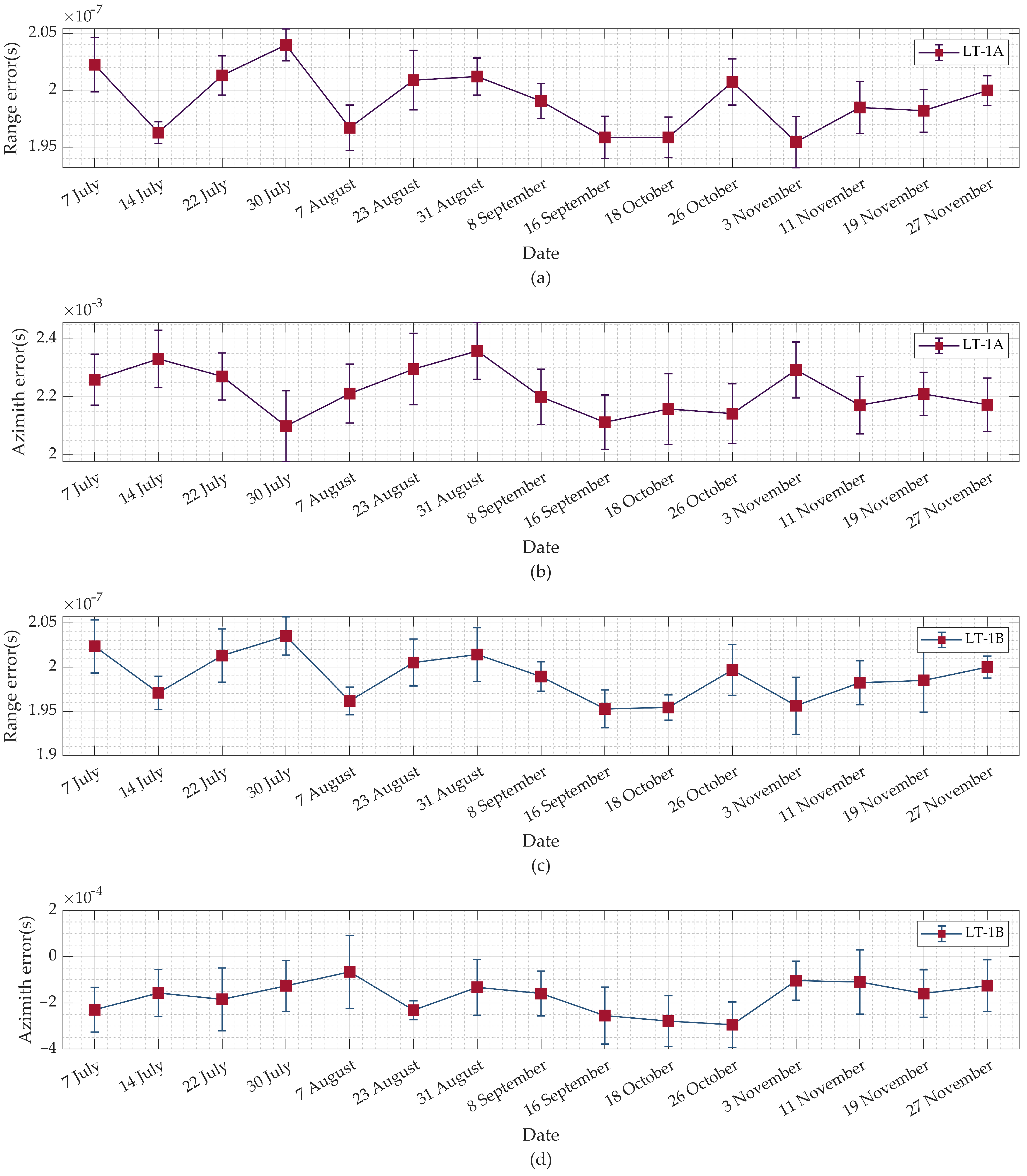
3.3.2. Systematic Error Determination

In this section, we compile the results of geometric calibration, as depicted in Figure 11. Each red dot in the graph represents the average error determined from the two test sites for a specific date, with error bars representing the STD of the daily results.
Figure 11a illustrates the range time error for the master SAR LT-1A. The range time error is stable from July to November, with a mean value of 199.078 ns and an STD of 2.658 ns. Figure 11c shows the range time error results for LT-1B, which maintains stability from July to November at 198.939 ns with an STD of 2.635 ns. Additionally, the daily range time error STD for both the master SAR and slave SAR remains within 3.5 ns.
Figure 11b displays the azimuth time error for the master SAR. Long-term monitoring reveals an average azimuth time error of 2.218 ms, with an STD of 0.076 ms. Figure 11d presents the azimuth time error for the slave SAR, with an average error of 0.174 ms and an STD of 0.066 ms over time.
Moreover, the geometric calibration accuracy of LT-1A and LT-1B are nearly identical. The reasons for this similarity are as follows: Firstly, the master and slave satellites have identical payloads, antennas, GNSS equipment, and other devices. Secondly, the external environment in which the master and slave satellites operate is nearly identical, resulting in similar environmental influences on the equipment. Lastly, in bistatic mode, the master and slave satellites undergo operations for time synchronization, beam synchronization, and phase synchronization. During the time synchronization procedure, a synchronization signal is employed to maintain synchronization between the timeline of the slave satellite and that of the master satellite. It is important to note that this synchronization process only applies to the range time and not to the azimuth time. Consequently, the range time errors for both the master and slave satellites are nearly identical, while the azimuth time errors differ. This conclusion is validated by the geometric calibration results in Figure 11.

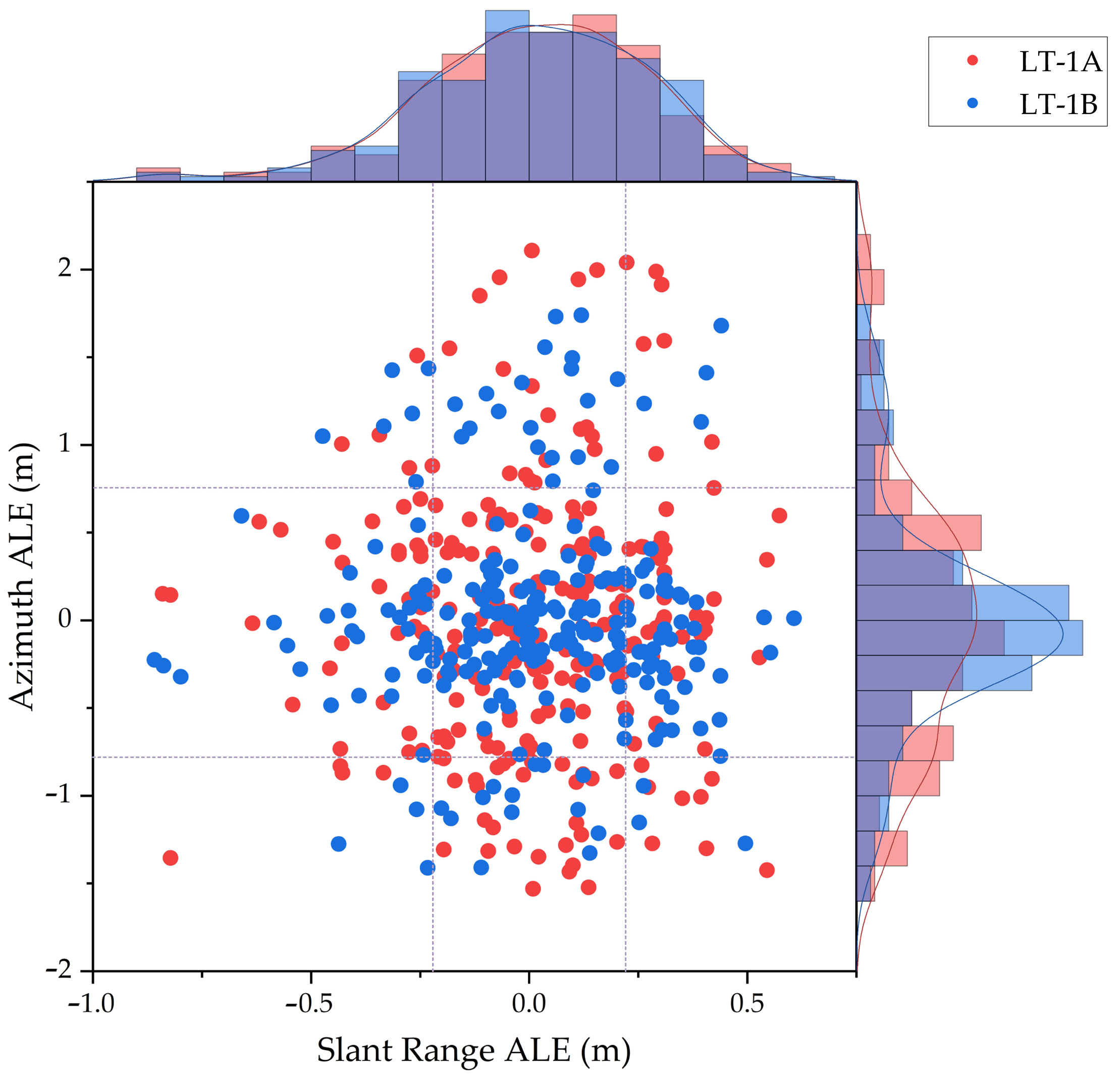
3.3.3. Absolute Location Error Derivation

Subsequently, we compensate for the initial azimuth and range time of master and slave SAR based on the average values of time errors. The ALE results for all CRs in the SLC data are depicted in Figure 12. As shown in the histogram and the dotted line in Figure 12, the STD of the azimuth and slant range ALE for LT-1A are 0.767 m and 0.229 m, respectively, corresponding to a planimetric geolocation error STD of 0.788 m (1 δ ). Similarly, the STD of azimuth and slant range ALE for LT-1B are 0.614 m and 0.228 m, respectively, with a corresponding planimetric geolocation error STD of 0.687 m (1 δ ). Furthermore, through the analysis of the error histogram, it can be observed that the error results exhibit a Gaussian-like distribution, indicating typical characteristics of the random error distribution. Thus, the systematic time errors have been effectively compensated for.
Therefore, the long-term error monitoring results of LT-1 demonstrate that both azimuth and range time errors meet the specified requirements. The systematic time error can be effectively compensated for during data processing, facilitating accurate geometric geolocation.

4. Discussion

In this section, we contrast the geolocation accuracy of LT-1 with that of existing L-band SAR systems, including ALOS-1 [14], ALOS-2 [15], SAOCOM-1A [44,45], and SAOCOM-1B [31].
Based on [43], the theoretical lower limit for identifying the location of the main lobe peak in a single SAR image observation (in length units) is as follows:
σ C R = 3 π 2 · 1 S N R · ρ r , a 0.39 S N R · ρ r , a
where S N R is the signal-to-noise ratio, and ρ r , a represents one of range or azimuth resolutions. Based on the existing literature, we list the related geolocation parameters of existing L-band SAR systems and calculate the ideal accuracy using Equation (30) in Table 4. Since the SNR of the CRs used for geolocation in ALOS-2, SAOCOM-1A, and SAOCOM-1B is unknown, we assume it to be the same as the SNR of the CRs used for LT-1, which is 20 dB, for our calculations.
According to Table 4, the ideal geolocation accuracy for ALOS-1, ALOS-2, SAOCOM-1A, SAOCOM-1B, and LT-1 are 1.54m, 0.48m, 0.51m, 0.51m, and 0.09m, respectively. LT-1’s geolocation accuracy surpasses other L-band SAR systems by more than an order of magnitude, primarily due to its high resolution.
According to published sources, ALOS-1 has a geometric accuracy of 9.7 m (root mean square) [14]. Similarly, ALOS-2 boasts a geometric accuracy of 10 m (root mean square) [15]. Concerning SAOCOM-1A, the geolocation error STD is noted at 1.8 m in azimuth and 18.1 m in the ground range, encompassing all beams and sites. A more focused analysis on the same beam and calibration site reveals an STD of 0.8 m in azimuth and 6.4 m in the ground range [44]. Transitioning to SAOCOM-1B, with an azimuth resolution of 6 m and a ground range resolution of 10 m, the azimuth and range ALE distribution spans from 20 m to 20 m, and 10 m to 10 m [31]. Here, we take one-third of the ALE peak value as the STD, which means SAOCOM-1B’s geolocation accuracy is 3.3 m in azimuth and 6.6 m in the range.
By comparison, the geometric geolocation results presented by LT-1 in Figure 12 reveal geolocation accuracies of 0.788 m and 0.687 m for LT-1A and LT-1B, which firmly establishes LT-1 as a benchmark in geometric accuracy exceeding the performance of eminent L-band SAR systems like ALOS-1, ALOS-2, SAOCOM-1A, and SAOCOM-1B. In addition, LT-1 has elevated the geolocation precision of L-band SAR systems from meter-level to decimeter-level accuracy, thus solidifying a promising status among these well-established L-band SAR systems.
However, it is imperative to acknowledge that these outcomes may vary depending on geographical location, imaging modes, image resolutions, and environmental conditions. This underscores the necessity for meticulous deliberation when interpreting and applying these geolocation accuracies for practical applications.
Moreover, it is vital to recognize that while geometric calibration is of utmost importance, the primary objective of LT-1 in bistatic mode is DEM production. Range time and azimuth time are essential inputs for subsequent DEM generation processes. For instance, the value of the slant range directly influences height accuracy, with a 30 m slant range error typically resulting in a height error of 15 to 30 m. Additionally, azimuth time errors can lead to discrepancies between the estimated and actual satellite positions. If the satellite’s velocity is 7.6 km/s, a 2 ms azimuth time error can result in a 15.2 m position estimation error, thus affecting the baseline vector derived from the subtraction of master and slave satellite vectors [46]. In cases with a 70 m ambiguous height, a 1 cm baseline error in the L-band biSAR system can introduce approximately 3 m of height error [33]. Consequently, interferometric processing to generate DEM is susceptible to geometric parameters. If geometric calibration is not performed before interferometric processing, the existing geometric errors of the master and slave satellites introduce a minimum height error of 30 m, whereas the height accuracy requirement for LT-1 is 5 m [42]. Future research endeavors will focus on integrating the outcomes of geometric calibration into subsequent interferometric procedures.

5. Conclusions

The objective of this study is to achieve geometric calibration for the LT-1 system. We analyzed the sources of geometric distortions, identifying the critical calibration parameters as the initial azimuth time and initial range time. Subsequently, we formulated geometric calibration models for LT-1A and LT-1B based on range and Doppler parameters. These models were solved through the minimization of the 2-norm of residuals approach. We selected two calibration sites in Xinjiang, China, where 16 CRs were deployed to validate the proposed calibration models.
Utilizing LT-1 data obtained on 8 September 2022, as sample data, we elaborated on the calibration process. The results from this sample data indicated that the mean range time errors for LT-1A and LT-1B were 197.610 ns and 198.010 ns, with STD of 2.161 ns and 1.975 ns, respectively, fulfilling the required precision of 5 ns. Similarly, the mean azimuth time errors for LT-1A and LT-1B were found to be 2.058 ms and −0.159 ms, accompanied by STD of 0.096 ms and 0.085 ms, respectively, in compliance with the 0.1 ms precision criteria.
Building upon these initial results, we conducted further geometric calibration verification using LT-1 image data from July to November, employing the same methodology. The mean range time errors for LT-1A and LT-1B were calculated as 199.078 ns and 198.939 ns, respectively, accompanied by STD of 2.658 ms and 2.635 ms, satisfying the 5 ns precision criterion. Similarly, the mean azimuth time errors for LT-1A and LT-1B were calculated as 2.218 ms and 0.174 ms, respectively, accompanied by STD of 0.076 ms and 0.066 ms, satisfying the 0.1 ms precision criterion.
Furthermore, the error results derived from geometric calibration were applied to enhance geometric geolocation accuracy. Consequently, planimetric geolocation errors for LT-1A and LT-1B exhibited STD of 0.767 m and 0.687 m (1 δ ), respectively. These outcomes affirm that both the sample data and the long-term monitoring results meet the geometric calibration requirements for LT-1, thereby enabling precise geometric geolocation.
Finally, we conducted a comparative analysis of LT-1’s geolocation results against existing L-band SAR systems. This comparison verified that LT-1 has elevated the polarimetric geolocation accuracy of L-band SAR systems from meter-level to decimeter-level precision. Moving forward, we focus on integrating the obtained geometric calibration results into subsequent interferometric calibration procedures for accurate DEM generation.

Author Contributions

Conceptualization, Y.W. (Yu Wang); data curation, A.W.; formal analysis, J.M. and G.L.; funding acquisition, Y.W. (Yu Wang); investigation, J.M., S.S. and G.L.; methodology, J.M.; project administration, J.H.; resources, A.W.; software, J.M.; supervision, J.H.; validation, J.M., Y.W. (Yu Wang), Y.W. (Yachao Wang) and S.S.; visualization, J.M.; writing—original draft, J.M. and Y.W. (Yu Wang); writing—review and editing, J.M. and Y.W. (Yu Wang). All authors will be informed about each step of manuscript processing including submission, revision, revision reminder, etc. via emails from our system or assigned Assistant Editor. All authors have read and agreed to the published version of the manuscript.

Funding

This research was funded by the National Natural Science Foundation of China under grant number 61771453.

Data Availability Statement

No new data were created or analyzed in this study. Data sharing is not applicable to this article.

Acknowledgments

The authors would like to express their gratitude to the anonymous reviewers, associate editor, and the engineers involved in the deployment of corner reflectors at the calibration site for their valuable contributions and support.

Conflicts of Interest

The authors declare no conflict of interest.

References

  1. Moreira, A.; Prats-Iraola, P.; Younis, M.; Krieger, G.; Hajnsek, I.; Papathanassiou, K.P. A tutorial on synthetic aperture radar. IEEE Geosci. Remote Sens. Mag. 2013, 1, 6–43. [Google Scholar] [CrossRef]
  2. Zhang, G.; Zhao, R.; Li, S.; Deng, M.; Guo, F.; Xu, K.; Wang, T.; Jia, P.; Hao, X. Stability analysis of geometric geolocation accuracy of YG-13 satellite. IEEE Trans. Geosci. Remote Sens. 2020, 60, 1–12. [Google Scholar] [CrossRef]
  3. Feng, Y.; Lei, Z.; Tong, X.; Xi, M.; Li, P. An Improved Geometric Calibration Model for Spaceborne Sar Systems with a Case Study of Large-Scale Gaofen-3 Images. IEEE J. Sel. Top. Appl. Earth Obs. Remote Sens. 2022, 15, 6928–6942. [Google Scholar] [CrossRef]
  4. Curlander, J.C. Location of spaceborne SAR imagery. IEEE Trans. Geosci. Remote Sens. 1982, GE-20, 359–364. [Google Scholar] [CrossRef]
  5. Wivell, C.; Steinwand, D.; Kelly, G.; Meyer, D. Evaluation of terrain models for the geocoding and terrain correction, of synthetic aperture radar (SAR) image. IEEE Trans. Geosci. Remote Sens. 2020, 30, 1137–1144. [Google Scholar] [CrossRef]
  6. Schubert, A.; Jehle, M.; Small, D.; Meier, E. Influence of Atmospheric Path Delay on the Absolute Geolocation Accuracy of TerraSAR-X High-Resolution Products. IEEE Trans. Geosci. Remote Sens. 2009, 48, 751–758. [Google Scholar] [CrossRef]
  7. Small, D.; Rosich, B.; Schubert, A.; Meier, E.; Nüesch, D. Geometric validation of low and high-resolution ASAR imagery. In Proceedings of the 2004 Envisat and ERS Symposium, ESA SP-572, Salzburg, Austria, 6–10 September 2004. [Google Scholar]
  8. Schubert, A.; Small, D.; Miranda, N.; Geudtner, D.; Meier, E. Sentinel-1A Product Geolocation Accuracy: Commissioning Phase Results. Remote Sens. 2015, 7, 9431–9449. [Google Scholar] [CrossRef]
  9. Gisinger, C.; Schubert, A.; Breit, H.; Garthwaite, M.; Balss, U.; Willberg, M.; Small, D.; Eineder, M.; Miranda, N. In-depth verification of Sentinel-1 and TerraSAR-X geolocation accuracy using the Australian corner reflector array. IEEE Trans. Geosci. Remote Sens. 2021, 59, 1154–1181. [Google Scholar] [CrossRef]
  10. Mohr, J.J.; Madsen, S.N. Geometric calibration of ERS satellite SAR images. IEEE Trans. Geosci. Remote Sens. 2001, 39, 842–850. [Google Scholar] [CrossRef]
  11. Zandbergen, R.; Dow, J.; Merino, M.R.; Píriz, R.; Fadrique, F.M. ERS-1 and ERS-2 tandem mission: Orbit determination, prediction and maintenance. Adv. Space Res. 1997, 19, 1649–1653. [Google Scholar] [CrossRef]
  12. Brautigam, B.; Schwerdt, M.; Bachmann, M.; Doring, B. Results from geometric and radiometric calibration of TerraSAR-X. In Proceedings of the 2007 European Radar Conference, EUSAR 2007, Munich, Germany, 17 December 2007; pp. 87–90. [Google Scholar]
  13. Schwerdt, M.; Brautigam, B.; Bachmann, M.; Doring, B.; Schrank, D.; Gonzalez, J.H. Final results of the efficient TerraSAR-X calibration method. In Proceedings of the 2008 IEEE Radar Conference, Rome, Italy, 26–30 May 2008; pp. 1–6. [Google Scholar]
  14. Shimada, M.; Isoguchi, O.; Tadono, T.; Isono, K. PALSAR radiometric and geometric calibration. IEEE Trans. Geosci. Remote Sens. 2009, 47, 3915–3932. [Google Scholar] [CrossRef]
  15. Motohka, T.; Isoguchi, O.; Sakashita, M.; Shimada, M. Results of ALOS-2 PALSAR-2 Calibration and Validation After 3 Years of Operation. In Proceedings of the 2018 IEEE International Geoscience and Remote Sensing Symposium, IGARSS 2018, Valencia, Spain, 22–27 July 2018; pp. 4169–4170. [Google Scholar]
  16. Schubert, A.; Miranda, N.; Geudtner, D.; Small, D. Sentinel-1A/B Combined Product Geolocation Accuracy. Remote Sens. 2017, 9, 607. [Google Scholar] [CrossRef]
  17. Williams, D.; LeDantec, P.; Chabot, M.; Hillman, A.; James, K.; Caves, R.; Thompson, A.; Vigneron, C.; Wu, Y. RADARSAT-2 image quality and calibration update. In Proceedings of the 10th European Conference on Synthetic Aperture Radar, 2014 EUSAR, Berlin, Germany, 3–5 June 2014; pp. 1–4. [Google Scholar]
  18. Zhao, R.; Zhang, G.; Deng, M.; Xu, K.; Guo, F. Geometric Calibration and Accuracy Verification of the GF-3 Satellite. Sensors 2017, 17, 1977–1989. [Google Scholar] [CrossRef] [PubMed]
  19. Walterscheid, I.; Ender, J.; Brenner, A.; Loffeld, O. Bistatic SAR processing and experiments. IEEE Trans. Geosci. Remote Sens. 2006, 44, 2710–2717. [Google Scholar] [CrossRef]
  20. Wang, R.; Deng, Y. Bistatic SAR System and Signal Processing Technology; Springer: Singapore, 2018. [Google Scholar]
  21. Mou, J.; Wang, Y.; Hong, J.; Wang, Y.; Wang, A. Baseline Calibration of L-Band Spaceborne Bistatic SAR TwinSAR-L for DEM Generation. Remote Sens. 2023, 15, 3024. [Google Scholar] [CrossRef]
  22. Jin, G.; Liu, K.; Liu, D.; Liang, D.; Zhang, H.; Ou, N.; Zhang, Y.; Deng, Y.; Li, C.; Wang, R. An advanced phase synchronization scheme for LT-1. IEEE Trans. Geosci. Remote Sens. 2020, 58, 1735–1746. [Google Scholar] [CrossRef]
  23. Liang, D.; Liu, K.; Yue, H.; Chen, Y.; Deng, Y.; Zhang, H.; Li, C.; Jin, G.; Wang, R. An advanced non-interrupted synchronization scheme for bistatic synthetic aperture radar. In Proceedings of the 2019 IEEE International Geoscience and Remote Sensing Symposium, IGARSS 2019, Yokohama, Japan, 28 July–2 August 2019; pp. 1116–1119. [Google Scholar]
  24. Zhang, Y.; Zhang, H.; Ou, N.; Liu, K.; Liang, D.; Deng, Y.; Wang, R. First demonstration of multipath effects on phase synchronization scheme for LT-1. IEEE Trans. Geosci. Remote Sens. 2019, 58, 2590–2604. [Google Scholar] [CrossRef]
  25. Xie, H.; Zhan, Y.; Zeng, G.; Pan, X. LEO mega-constellations for 6G global coverage: Challenges and opportunities. IEEE Access 2021, 9, 164223–164244. [Google Scholar] [CrossRef]
  26. Zink, M.; Bachmann, M.; Brautigam, B.; Fritz, T.; Hajnsek, I.; Moreira, A.; Wessel, B.; Krieger, G. TanDEM-X: The new global DEM takes shape. IEEE Geosci. Remote Sens. Mag. 2014, 2, 8–23. [Google Scholar] [CrossRef]
  27. Rossi, C.; Gonzalez, F.R.; Fritz, T.; Yague-Martinez, N.; Eineder, M. TanDEM-X calibrated raw DEM generation. ISPRS J. Photogramm. Remote Sens. 2012, 73, 12–20. [Google Scholar] [CrossRef]
  28. Krieger, G.; Moreira, A.; Fiedler, H.; Hajnsek, I.; Werner, M.; Younis, M.; Zink, M. TanDEM-X: A satellite formation for high-resolution SAR interferometry. IEEE Trans. Geosci. Remote Sens. 2007, 45, 3317–3341. [Google Scholar] [CrossRef]
  29. Scipal, K.; Davidson, M. The SAOCOM-CS mission: ESA’s first bistatic and tomographic L-band mission. In Proceedings of the 2017 IEEE International Geoscience and Remote Sensing Symposium. IGARSS 2017, Fort Worth, TX, USA, 23–28 July 2017; pp. 123–124. [Google Scholar]
  30. González, J.H.; Antony, J.M.W.; Bachmann, M.; Krieger, G.; Zink, M.; Schrank, D.; Schwerdt, M. Bistatic system and baseline calibration in TanDEM-X to ensure the global digital elevation model quality. ISPRS J. Photogramm. Remote Sens. 2012, 73, 3–11. [Google Scholar] [CrossRef]
  31. Fioretti, L.; Giudici, D.; Guccione, P.; Recchia, A.; Steinisch, M. SAOCOM-1B Independent Commissioning Phase Results. In Proceedings of the 2021 IEEE International Geoscience and Remote Sensing Symposium. IGARSS 2021, Brussels, Belgium, 11–16 July 2021; pp. 1757–1760. [Google Scholar]
  32. Ding, C.; Liu, J.; Lei, B.; Qiu, X. Preliminary exploration of systematic geolocation accuracy of GF-3 SAR satellite system. J. Radars 2017, 6, 11–16. [Google Scholar]
  33. Antony, J.M.W.; Gonzalez, J.H.; Schwerdt, M.; Bachmann, M.; Krieger, G.; Zink, M. Results of the TanDEM-X Baseline Calibration. IEEE J. Sel. Top. Appl. Earth Obs. Remote. Sens. 2013, 6, 1495–1501. [Google Scholar] [CrossRef]
  34. Mendes, V.B.; Langley, R.B. Tropospheric zenith delay prediction accuracy for airborne GPS high-precision geolocation. In Proceedings of the Institute of Navigation 54th Annual Meeting, Denver, CO, USA, 1–3 June 1998; pp. 337–347. [Google Scholar]
  35. Yu, C.; Li, Z.; Penna, N.T.; Crippa, P. Generic atmospheric correction model for interferometric synthetic aperture radar observations. J. Geophys. Res. Solid Earth 2018, 123, 9202–9222. [Google Scholar] [CrossRef]
  36. Yu, C.; Li, Z.; Penna, N.T. Interferometric synthetic aperture radar atmospheric correction using a GPS-based iterative tropospheric decomposition model. Remote Sens. Environ. 2018, 204, 109–121. [Google Scholar] [CrossRef]
  37. Yu, C.; Penna, N.T.; Li, Z. Generation of rea-time mode high-resolution water vapor fields from GPS observations. J. Geophys. Res. Atmos. 2017, 122, 2008–2025. [Google Scholar] [CrossRef]
  38. Berrada Baby, H.; Gole, P.; Lavergnat, J. A model for the tropospheric excess path length of radio waves from surface meteorological measurements. Radio Sci. 1988, 23, 1023–1038. [Google Scholar] [CrossRef]
  39. Jehle, M.; Perler, D.; Small, D.; Schubert, A.; Meier, E. Estimation of atmospheric path delays in TerraSAR-X data using models vs. measurements. Sensors 2008, 8, 8479–8491. [Google Scholar] [CrossRef]
  40. Zhang, G.; Fei, W.-B.; Li, Z.; Zhu, X.; Li, D.-R. Evaluation of the RPC model for spaceborne SAR imagery. Photogramm. Eng. Remote Sens. 2010, 76, 727–733. [Google Scholar] [CrossRef]
  41. Zhang, L.; Balz, T.; Liao, M. Satellite SAR geocoding with refined RPC model. ISPRS J. Photogramm. Remote Sens. 2012, 69, 37–49. [Google Scholar] [CrossRef]
  42. Qi, Y.; Wang, Y.; Hong, J.; Du, S. Additional Reference Height Error Analysis for Baseline Calibration Based on a Distributed Target DEM in TwinSAR-L. Remote Sens. 2021, 13, 2750. [Google Scholar] [CrossRef]
  43. Schubert, A.; Small, D.; Gisinger, C.; Balss, U.; Eineder, M. Corner Reflector Deployment for SAR Geometric Calibration and Performance Assessment. ESRIN: Frascati 2018, 1.03, 14–17. [Google Scholar]
  44. Azcueta, M.; Gonzalez, J.P.C.; Zajc, T.; Ferreyra, J.; Thibeault, M. External Calibration Results of the SAOCOM-1A Commissioning Phase. IEEE Trans. Geosci. Remote Sens. 2022, 60, 1–8. [Google Scholar] [CrossRef]
  45. Anconitano, G.; Acuña, M.A.; Guerriero, L.; Pierdicca, N. Analysis of Multi-Frequency SAR Data for Evaluating Their Sensitivity to Soil Moisture Over an Agricultural Area in Argentina. In Proceedings of the 2022 IEEE International Geoscience and Remote Sensing Symposium, 2022 IGARSS, Kuala Lumpur, Malaysia, 17–22 July 2022; pp. 5716–5719. [Google Scholar]
  46. Lu, R.; Wen, J.; Zhao, D.; Liu, Y.; Hou, Y.; Chen, C. Analysis of Influencing Factors of Distributed Satellite InSAR Height-Measurement Accuracy based on Positioning Equation. In Proceedings of the 2022 3rd China International SAR Symposium (CISS), Shanghai, China, 2–4 November 2022; pp. 1–8. [Google Scholar]
Figure 1. Sources of geometric distortions. (a) Sensor error. (b) Bistatic azimuth shift. (c) Solid Earth tidal displacement. (d) Ephemeris error of platform. (e) Atmospheric path delay.
Remotesensing 15 05280 g001
Figure 2. Observation scheme of the master SAR.
Remotesensing 15 05280 g002
Figure 3. Observation scheme of the slave SAR.
Remotesensing 15 05280 g003
Figure 4. Workflow of the geometric calibration method.
Remotesensing 15 05280 g004
Figure 5. Diagram illustrating the location of corner reflectors. (a) Test site A. (b) Test site B.
Remotesensing 15 05280 g005
Figure 6. Atmospheric path delay. (a) Test site A. (b) Test site B.
Remotesensing 15 05280 g006
Figure 7. (a) The precise positions of the corner reflectors on the test site A. (b) Enlarged views of the first CR. (c) Upsampled amplitude map of (b).
Remotesensing 15 05280 g007
Figure 8. (a) The precise positions of the CRs on the test site B. (b) Enlarged views of the first CR. (c) Upsampled amplitude map of (b).
Remotesensing 15 05280 g008
Figure 9. Geometric calibration results of the selected SAR image. (a) Range time error of LT-1A. (b) Azimuth time error of LT-1A. (c) Range time error of LT-1B. (d) Azimuth time error of LT-1B.
Remotesensing 15 05280 g009
Figure 10. Atmospheric path delay of two test sites from 7 July 2022 to 27 November 2022.
Remotesensing 15 05280 g010
Figure 11. The long-term monitoring results of geometric calibration. (a) Range time error of LT-1A. (b) Azimuth time error of LT-1A. (c) Range time error of LT-1B. (d) Azimuth time error of LT-1B.
Remotesensing 15 05280 g011
Figure 12. ALE of CRs after geometric calibration.
Remotesensing 15 05280 g012
Table 1. SceneID of selected LT-1 SAR images for validating the geometric calibration model.
Date7 July 202214 July 202222 July 202230 July 20227 August 2022
Test site A26,74728,31328,89129,60730,279
Test site B26,75228,31128,89029,60630,278
Date23 August 202231 August 20228 September 202216 September 202218 October 2022
Test site A32,57233,61634,69636,06642,603
Test site B32,57031,61834,69536,06542,601
Date26 October 20223 November 202211 November 202219 November 202227 November 2022
Test site A44,73546,50448,11749,96051,498
Test site B44,74046,50348,12249,95951,501
Table 2. Parameters of the data acquired on 8 September 2022.
Test Site ATest Site B
MasterSlaveMasterSlave
SceneID34,69634,69634,69534,695
OrbitID3365288733652887
Incidence Angle44.496°44.365°22.440°22.342°
Azimuth Spacing1.995 m1.995 m1.769 m1.769 m
Range Spacing1.665 m1.665 m1.665 m1.665 m
Dimension27,280 × 22,91427,320 × 22,91437,692 × 12,67437,756 × 12,674
Table 3. Statistical results of time errors and geolocation errors in two sites.
LT-1ALT-1B
Slant RangeAzimuthSlant RangeAzimuth
34,69634,69534,69634,69534,69634,69534,69634,695
Time errorMean198.337 ns196.876 ns2.056 ms2.061 ms198.864 ns197.149 ns−0.242 ms−0.075 ms
STD1.574 ns1.587 ns0.137 ms0.032 ms1.881 ns1.254 ns0.112 ms0.026 ms
Total197.610 ± 2.161 ns2.058 ± 0.096 ms198.010 ± 1.975 ns−0.159 ± 0.085 ms
ALEMean29.730 m29.511 m−15.711 m−15.742 m29.809 m29.552 m−15.504 m−16.113 m
STD0.236 m0.238 m1.054 m0.249 m0.282 m0.188 m0.542 m0.233 m
Total29.621 ± 0.324 m−15.726 ± 0.740 m29.681 ± 0.296 m−1.208 ± 0.512 m
Table 4. Each system’s geolocation parameters in strip mode.
SatelliteALOS-1ALOS-2SAOCOM-1ASAOCOM-1BLT-1
Range resolution4.5 m6 m12 m12 m1.7 m
Azimuth resolution8.9 m6 m6 m6 m2 m
SNR8 dBNot mentionedNot mentionedNot mentioned20 dB
Ideal range accuracy0.69 m0.34 m0.46 m0.46 m0.06 m
Ideal azimuth accuracy1.38 m0.34 m0.23 m0.23 m0.07 m
Ideal ALE1.54 m0.48 m0.51 m0.51 m0.09 m
Actual ALE9.7 m10 m0.8 m × 6.4 m3.3 m × 6.6 m0.76 m × 0.23 m
Disclaimer/Publisher’s Note: The statements, opinions and data contained in all publications are solely those of the individual author(s) and contributor(s) and not of MDPI and/or the editor(s). MDPI and/or the editor(s) disclaim responsibility for any injury to people or property resulting from any ideas, methods, instructions or products referred to in the content.

