A Neural Network for Hyperspectral Image Denoising by Combining Spatial–Spectral Information

Abstract

Hyperspectral imaging often suffers from various types of noise, including sensor non-uniformity and atmospheric disturbances. Removing multiple types of complex noise in hyperspectral images (HSIs) while preserving high fidelity in spectral dimensions is a challenging task in hyperspectral data processing. Existing methods typically focus on specific types of noise, resulting in limited applicability and an inadequate ability to handle complex noise scenarios. This paper proposes a denoising method based on a network that considers both the spatial structure and spectral differences of noise in an image data cube. The proposed network takes into account the DN value of the current band, as well as the horizontal, vertical, and spectral gradients as inputs. A multi-resolution convolutional module is employed to accurately extract spatial and spectral noise features, which are then aggregated through residual connections at different levels. Finally, the residual mixed noise is approximated. Both simulated and real case studies confirm the effectiveness of the proposed denoising method. In the simulation experiment, the average PSNR value of the denoised results reached 31.47 at a signal-to-noise ratio of 8 dB, and the experimental results on the real data set Indian Pines show that the classification accuracy of the denoised hyperspectral image (HSI) is improved by 16.31% compared to the original noisy version.

1. Introduction

Hyperspectral cameras have become increasingly popular in environmental monitoring due to their ability to capture continuous spectral bands and high spectral resolution. These cameras provide both spatial and spectral information of objects on the ground [1], making them valuable for applications, such as mineral exploration [2,3], food hygiene [4,5,6], and feature classification [7]. However, hyperspectral images are prone to noise interference caused by factors, such as sensor non-uniformity, atmospheric disturbances, and variations in lighting conditions [8,9]. This noise can significantly affect the image quality, especially in spectral bands with weak signal-to-noise ratios, limiting the utility of hyperspectral data [10,11,12,13].

The research on hyperspectral image denoising algorithms can be broadly categorized into two main approaches: model-based optimization methods and data-driven methods.

Model-based methods [14,15,16,17] aim to transform the problem of image quality improvement into a mathematically modelable optimization problem by analyzing the degradation process and utilizing prior knowledge of an ideal image. These methods typically involve iterative algorithms to achieve various image processing objectives. For example, Yuan et al. [14] proposed a spatial–spectral total variational method that adaptively denoises images by adjusting parameters to distinguish between high-intensity and low-intensity noise. Maggioni et al. [15] utilized local and non-local pixel correlations to stack pixel cubes and remove noise. Zhang et al. [16] exploited the spectral correlations between adjacent pixels and incorporated low-rank matrix characteristics for hyperspectral image recovery. However, these methods often require manual parameter tuning and can become computationally complex due to the large amount of data involved.

The other category of methods for hyperspectral image denoising are data-driven approaches, particularly deep learning methods [18,19,20,21]. These methods involve designing a differentiable multi-layer neural network model that includes convolutional layers and other structures. They make use of a large amount of training image data and optimize the network’s parameters through the back-propagation of surface parameter gradients. A pre-trained model based on a neural network is obtained, which is then applied to collected images for forward inference to achieve various purposes related to image quality improvement [22,23].

Data-driven methods, such as deep learning, have the advantage of utilizing a vast amount of existing data to capture image characteristics that are difficult to describe with strict mathematical models. As a result, they can achieve excellent performance when dealing with complex semantic problems. For instance, Chang et al. [24] introduced a deep convolutional neural network specifically for hyperspectral image denoising, although it was only suitable for noise removal in a specific number of bands. Yuan et al. [25] proposed a deep residual denoising convolutional neural network that achieved good results in removing Gaussian noise from HSIs using multi-scale and multi-level feature representations. Li et al. [26] proposed an HSI denoising method based on multi-resolution-gated networks using wavelet transform. Dong et al. [27] proposed an improved three-dimensional U-Net structure that leveraged the spatial–spectral correlation of HSIs, although it increased the computational requirements of the convolutional neural network.

In summary, existing HSI denoising methods have limitations in addressing specific noise problems and in effectively utilizing the spatial and spectral characteristics of hyperspectral images. While they can achieve certain results, they lack versatility and struggle with removing mixed noise. To overcome these limitations, this paper proposes a neural network approach for mixed noise removal from hyperspectral images by leveraging both spatial and spectral information. The contributions of this paper can be summarized as follows:

(1)

It is a consideration of the spatial–spectral correlation of hyperspectral images and the use of a neural network with multi-resolution convolutional modules to capture the spatial and spectral characteristics of objects and their surroundings.

(2)

It is a proposal of a loss function that balances the spatial and spectral structure of hyperspectral images, suppressing spectral distortion while preserving spatial structure information.

(3)

The proposed method is not specific to any particular detector and remains effective for wavelengths with poor image quality.

The remainder of this article is organized as follows. Section 2 presents the proposed methodology and the network structure used. Section 3 describes the data set and provides an analysis of the results obtained in simulations and real experiments and compares the proposed method with other methods. In addition, it details the ablation experiments, illustrating the effectiveness of the proposed method. Finally, the article is summarized in Section 4.

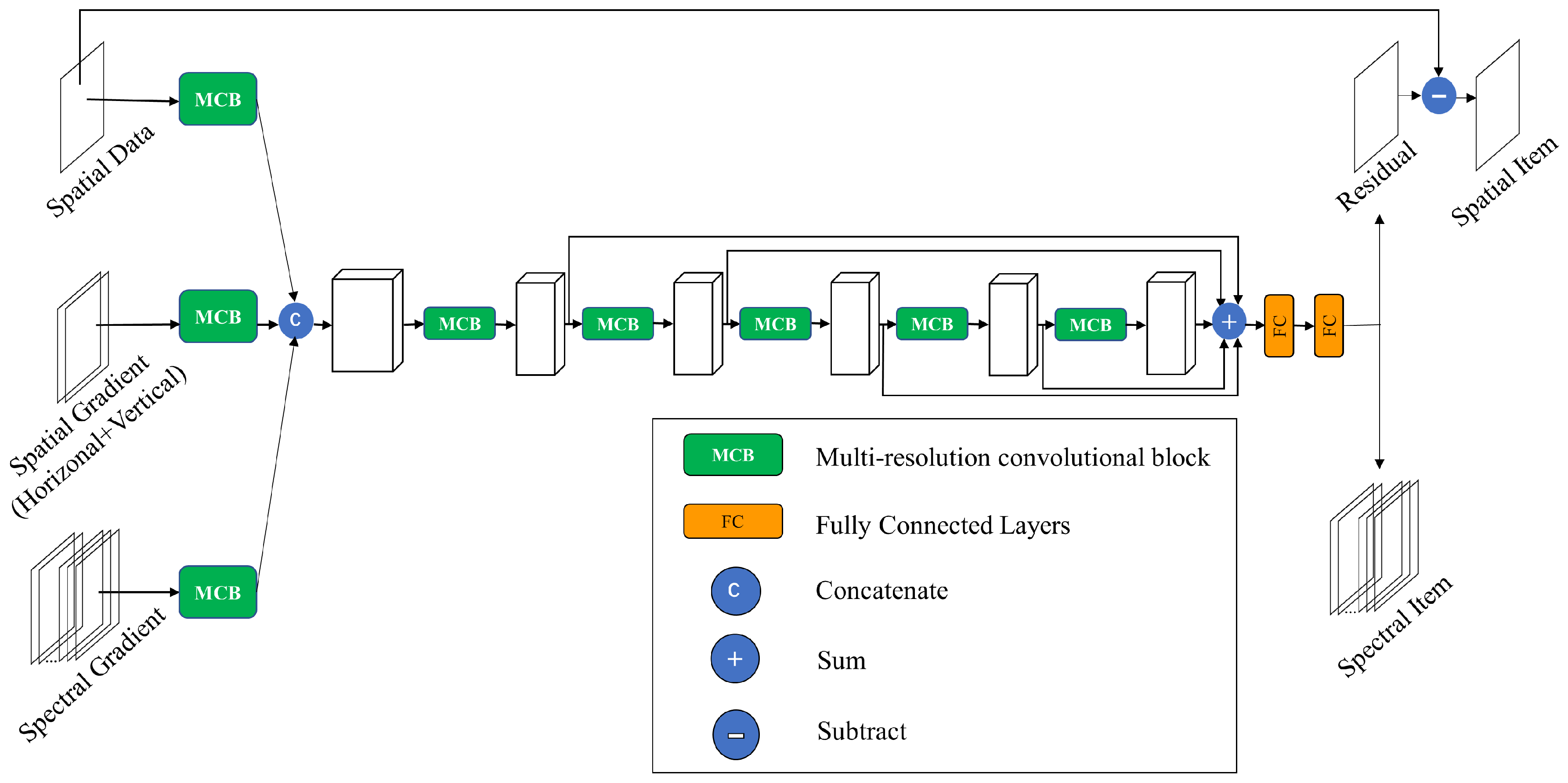
2. Spatial–Spectral Denoising Network

A hyperspectral image is a set of three-dimensional data of size $h\times w\times c$, where $h$ and $w$ represent the height and width of the HSI and $c$ represents the number of spectral bands. The HSI degradation model can be expressed as follows:

$$Y=X+N,$$

(1)

where $X$ represents the true image, $N$ represents noise, and $Y$ represents the image in which the noise can be observed. $X$ and $N$ have the same three-dimensional matrix size as $Y$, and the degradation model can also be expressed as $X=Y-N$. Thus, hyperspectral image denoising consists of subtracting the additive noise $N$ from a known noisy image $Y$, thereby restoring the clean image $X$.

The HSI denoising network proposed in this study is depicted in Figure 1. To fully consider the spatial and spectral correlations of hyperspectral images, the noisy band, its horizontal and vertical gradients, and the spectral gradient of adjacent bands were selected as the input for the network. The features were extracted through convolution at different resolutions, and the fully cascaded network was used to learn the features at different receptive field sizes. Residual connections used multiple feature mappings obtained from the intermediate connection layers. Finally, the residual mixed noise could be approximated, and the estimated noise result $N$ was subtracted from the input noise-polluted image $Y$ to obtain the denoised HSI $X$. HSI noise data with a size of $h\times w\times c$ were used as input during the test, and denoised images of the same size were directly restored by traversing all bands sequentially.

(1)

Spatial–spectral information acquisition module

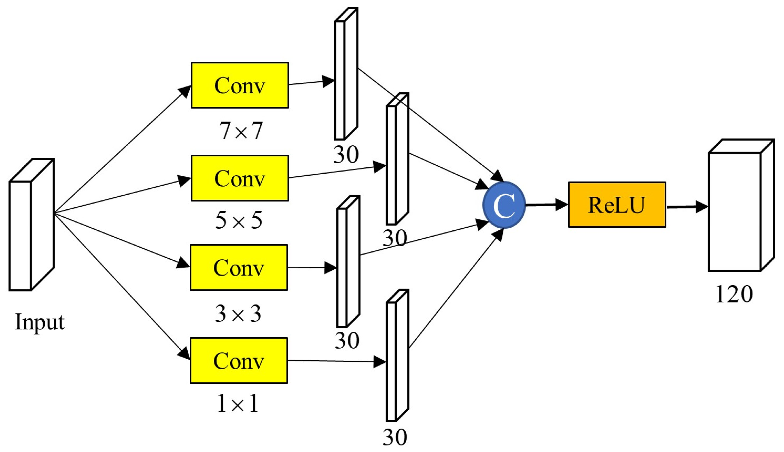
Due to its unique directional structure, spatial gradient information can effectively highlight sparse noise to a certain extent. Hyperspectral images contain rich spectral information, and each band’s noise level and noise type usually differ, providing additional complementary information. Thus, it was significant to fully use both spatial and spectral gradient information when performing HSI denoising.

The spatial gradient information used in this study was calculated using a Sobel filter with a horizontal filter $f_h$ and a vertical filter $f_v$. Convolution was performed among $f_h$, $f_v$, and the input image $Y$, and the horizontal gradient $S_h$ and vertical gradient $S_v$ were obtained as follows:

$$S_h=f_h*Y,$$

(2)

$$S_v=f_v*Y,$$

(3)

where $f_h$ and $f_v$ were represented as follows:

$$f_h=\left[\begin{array}{ccc}-1& 0& 1\\ -2& 0& 2\\ -1& 0& 1\end{array}\right],$$

(4)

$$f_v=\left[\begin{array}{ccc}-1& -2& -1\\ 0& 0& 0\\ 1& 2& 1\end{array}\right].$$

(5)

The spectral gradient could be expressed as follows:

$$S_s=Y(m,n,k+1)-Y(m,n,k),$$

(6)

where $m,n,k$ represented pixel coordinates in the three-dimensional hyperspectral image $Y$. The spatial–spectral information $F$ of the final network input could be represented as follows:

$$F=\left\{Y_k,S_h,S_v,S_s\right\}$$

(7)

where $Y_k$ was the noise map input for the current band $k$.

(2)

Multi-resolution convolutional module (MCB)

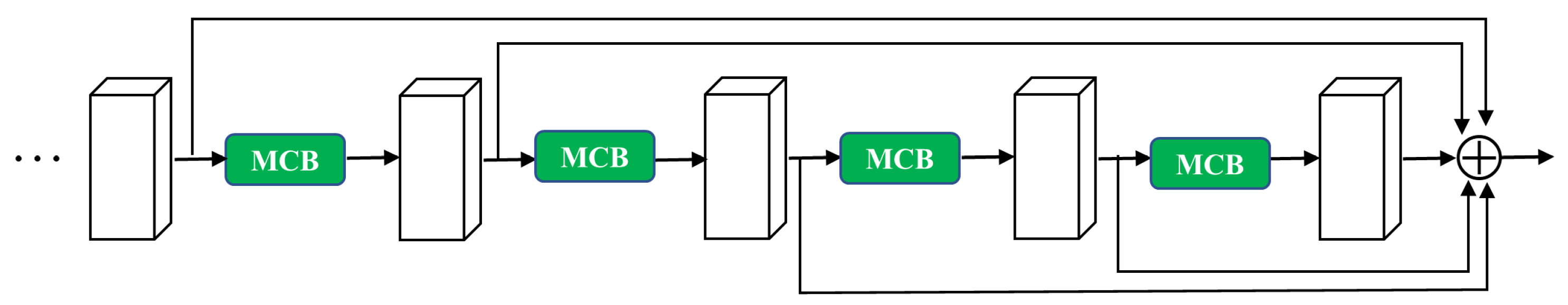
Regarding fringes and deadline noise, multi-resolution convolutional blocks were introduced to extract the multi-resolution features of contextual information, which can be used to obtain better information about objects and the surrounding environment. The receptive field of the network represents the size of the local area on the input image that will be mapped to depth features. Local features with small receptive fields contain more detailed information, and global features with large receptive fields can provide important contextual information for heavy noise removal, according to the non-local self-similarity (NSS) [28]. As shown in Figure 2, four convolution kernel sizes ($7\times 7$, $5\times 5$, $3\times 3$, and $1\times 1$) were applied to the spatial data, spatial gradients, and spectral gradients to obtain feature maps for 30 channels. For image recovery tasks, the input and output sizes must be consistent. Under the premise that the stride length is fixed at 1, in order to keep the output size the same size as the input size after convolution, the convolution operation corresponds to different fill values for convolution kernels of different resolutions. For convolution kernels of $3\times 3$, $5\times 5$, and $7\times 7$, the fill sizes are 1, 2, and 3, respectively. Various activation functions can be used in the non-linear activation layer, such as the tanh, sigmoid, and rectified linear unit (ReLU) functions. The ReLU activation function was chosen for this study considering the learning speed.

(3)

Multi-level feature representation

In this study, a fully cascaded multi-resolution convolution was used. The input features of each MCB were obtained by cascading the output features of all previous MCBs. Neural networks can usually take advantage of high nonlinearity to obtain more basic feature extraction and expression capabilities, and different feature information is present at different levels of depth. To effectively use the features between the indirect connection layers instead of direct attenuation, residual connections were used to concatenate the multiple feature maps from different convolutional layers, as shown in Figure 3. Residual connections can effectively reduce the degradation problem of traditional deep networks, so that we could add more training layers to the network and increase network performance.

(4)

Loss function

For the denoising and recovery of hyperspectral images, preservation of the spectral dimension must be considered as it is important for subsequent applications, such as object detection and demixing. In order to maintain the resilience of both the spatial and spectral dimensions of hyperspectral images, the following loss function was designed:

$$L=\left(1-\lambda \right)L_{spa}+\frac{\lambda }{2}{L}_{spe}+\frac{\lambda }{2}{L}_{d_{spe}},$$

(8)

where $L_{spa}$ was the loss in the spatial dimension; $L_{spe}$ was a loss in the spectral dimension before and after denoising the $K$ bands around it; $L_{d_{spe}}$ was also a loss in the spectral dimension, used to keep the gradient smooth after denoising the $K$ bands around it; and $\lambda$ was a hyperparameter that could balance the losses. We believe that $L_{spe}$ and $L_{d_{spe}}$ should have the same weight; as a rule of thumb, $\lambda =0.001$ was set in this study. A more detailed explanation of the loss functions is provided below:

$$\begin{array}{c}{L}_{spa}=\frac{1}{2T}{\displaystyle {\displaystyle \sum }_{i=1}^T}{\Vert Re{s}_k^i-\left(Y_k^i-X_k^i\right)\Vert }_2^2\end{array},$$

(9)

$$\begin{array}{c}{L}_{spe}=\frac{1}{2T}{\displaystyle {\displaystyle \sum }_{i=1}^T}{\Vert \left(S_s\left(X_z^i+Re{s}_z^i\right)\right)-\left(S_s\left(Y_z^i\right)\right)\Vert }_2^2\end{array},$$

(10)

$$\begin{array}{c}{L}_{d_{spe}}=\frac{1}{2T}{\displaystyle {\displaystyle \sum }_{i=1}^T}{\Vert \left(S_s\left(Y_z^i-Re{s}_z^i\right)\right)-Zer{o}_z^i\Vert }_2^2\end{array}.$$

(11)

In Equation (9), $T$ was the number of training blocks, $Re{s}_k^{}$ was the estimated residual output of the $k$th band, and $X_k$ was the $k$th band without added noise. $X_z$ in Equation (10) represented the $K$ bands around $X_k$, $Re{s}_z$ was the residual noise output of the $K$ bands around the current denoising band $Y_k$, $Y_z$ represented the $K$ bands around the current denoising band $Y_k$, and $S_s(\cdot )$ meant to find the spectral gradient according to Equation (6), so $S_s\left(Y_z\right)$ indicated that the spectral gradient was obtained for $Y_z$ according to Equation (6). In Equation (11), $S_s\left(Y_z^i-Re{s}_z^i\right)$ was the spectral gradient obtained for $Y_z^i-Re{s}_z^i$ according to Equation (6) and $Zer{o}_z$ was used to smooth the spectral gradient of the current band after denoising to zero, which was an all-zero matrix with the same size as $S_s\left(Y_z^i-Re{s}_z^i\right)$.

3. Experiments and Analysis

To verify the effectiveness of the proposed method against mixed noise in hyperspectral images, simulated and real data were utilized. The proposed method was compared with lower rank tensor approximation (LRTA) [29], block-matching and 4-D filtering (BM4D) [15], low-rank total variation (LRTV) [30], low-rank matrix recover (LRMR) [16], noise adjusted iterative low-rank matrix approximation (NAILRMA) [31], and spatial–spectral gradient network (SSGN) [32]. The average peak signal-to-noise ratio (MPSNR), mean structural similarity index (MSSIM), and mean spectral angle (MSAM) were used as evaluation indicators in the simulation experiments [25]. The MPSNR and MSSIM values reflect the similarity between two images according to their spatial structure, while the MSAM indicates the similarity in terms of the spectral dimension. In general, in simulation tests, the higher the MPSNR and MSSIM values are and the lower the MSAM value is, the better the HSI denoising effect is. Two hyperspectral images were tested in the experiment with actual data, and the average DN results for all columns are shown.

3.1. Experimental Setup

(1)

Test data set: Three data sets were used for the simulation and real data experiments.

(a)

The first data set was the image of the Washington DC Mall for the simulation experiments, with dimensions of 200 × 200 × 191.

(b)

The second data set was a 145 × 145 Indian Pines HSI taken with the Airborne Visible Infrared Imaging Spectrometer (AVIRIS), used for the real-data experiments. After removing bands heavily disturbed by the atmosphere and water, 198 bands were used for these experiments.

(c)

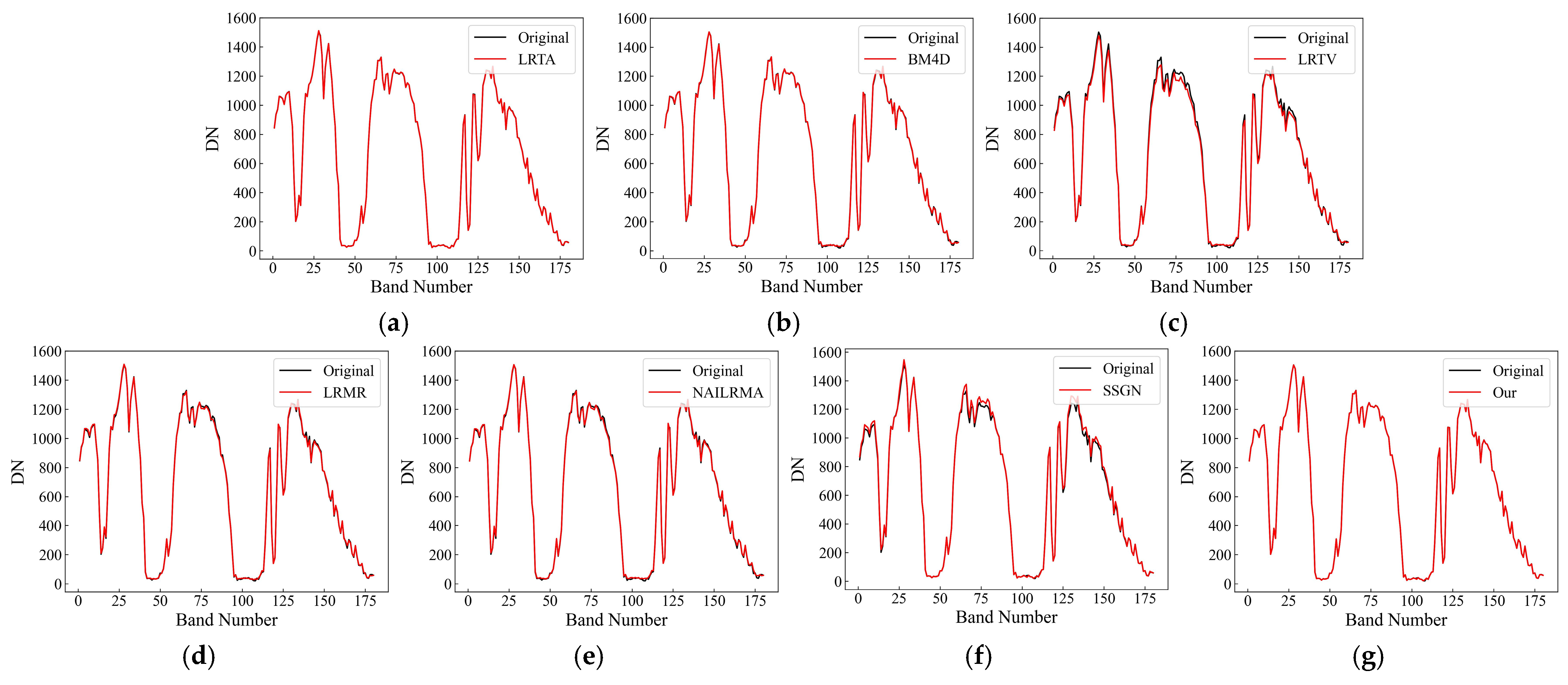
The third data set was an image acquired with the Gaofen-5 hyperspectral satellite AHSI payload, developed by the Shanghai Institute of Technical Physics, Chinese Academy of Sciences [33], with 180 spectral channels in the shortwave infrared band. An image of size 400 × 200 × 180 was captured for the experiments with real data.

(2)

Operating environment: All algorithms involved in this study were run in MATLAB R2019b based on the Pytorch 1.12.1 deep learning framework. The CPU processor was an Intel(R) Xeon(R) Gold 5218 [email protected] GHz, and an NVIDIA GeForce RTX 3090 GPU graphics card was used.

(3)

Training setup: An image of the Washington DC Mall with dimensions of 1280 × 303 × 191 was acquired using onboard HYDICE sensors. It was cropped to a sub-image of 200 × 200 × 191 to test the models, and the rest were used to train the network. The data of the trained network were normalized to [0–1] before the experiment. The slice size of the training data set was 25 × 25, the sampling step was 25, and the data were rotated and folded from multiple angles. In total, 437,007 true image slices were generated. The whole training process comprised a total of 300 epochs, with each epoch containing 200 iterations and each iteration involving 128 noise–truth slice sets. The training process for the proposed model costs roughly 11 h 30 min.

(4)

Parameter settings: In the simulations and experiments with actual data, the number of adjacent bands of the proposed model was set to K = 24, the trade-off parameter was set to α = 0.001, the Adam optimization algorithm was used as the gradient descent optimization method, and the momentum parameters were set to 0.9, 0.999, and 10⁻⁸, respectively. The learning rate was initialized to 0.001, and every 50 generations, the learning rate was reduced by multiplying by a factor of 0.5.

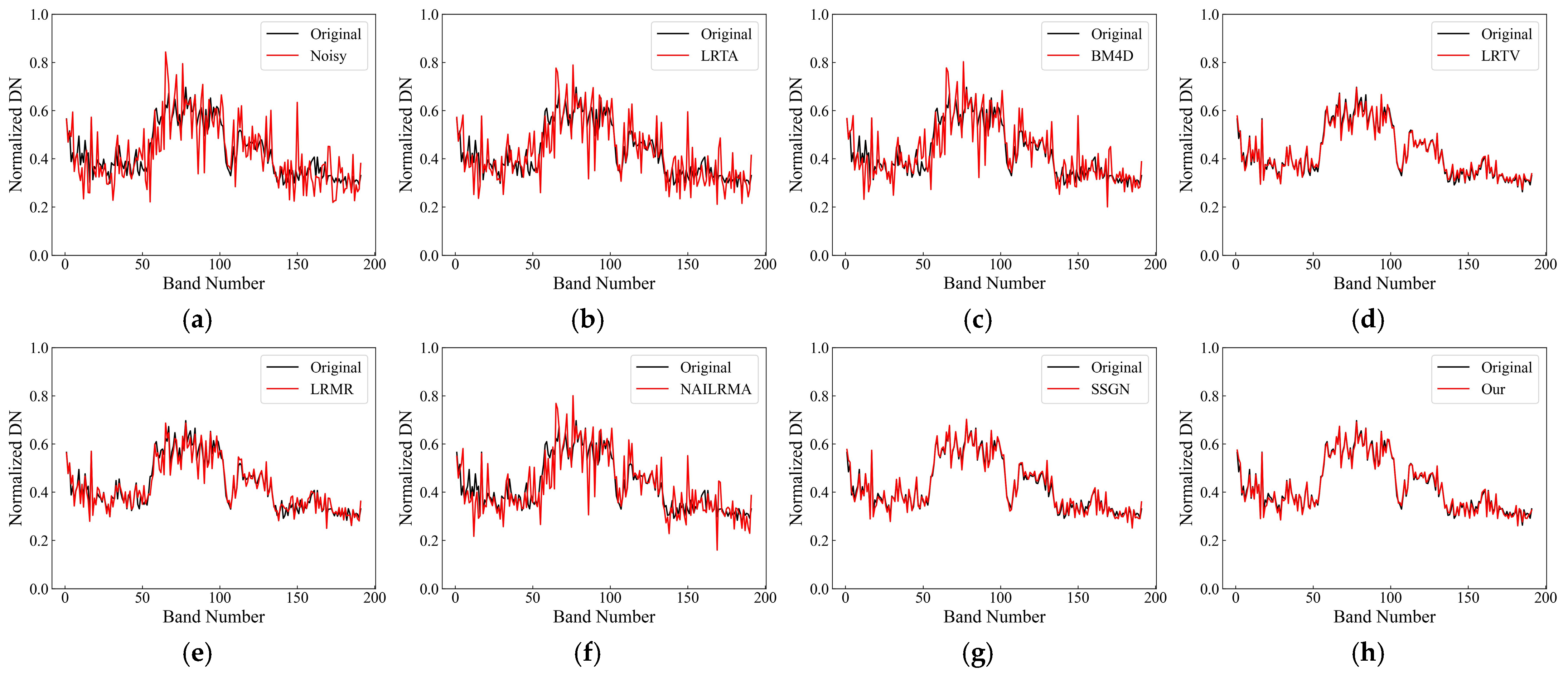
3.2. Simulation Experiments

In the hybrid noise reduction process for HSIs, we simulated the following five cases with additional noise.

Case 1 (Gaussian noise): Gaussian noise was added to all bands in the HSIs. The noise intensity differed for different bands and followed a random probability distribution.

Case 2 (stripe noise): All bands of the HSIs were contaminated by stripe noise. In the experiment, analog stripe noise was applied to all bands of the raw data. The simulated striping strategy was to randomly select columns in the original bands, half of which were increased with the intensity of the mean. In contrast, the remaining half were reduced with the intensity of the mean.

Case 3 (Gaussian noise + stripe noise): All bands in the HSIs were contaminated by Gaussian noise, and some bands were destroyed by stripe noise. The Gaussian noise intensity and band noise were the same as those in cases 1 and 2, respectively.

Case 4 (Gaussian noise + deadline noise): All bands in the HSIs were contaminated by Gaussian noise, and some bands were contaminated by deadline noise. Rows randomly selected from the 20 bands of the original data were treated as deadlines, while the Gaussian noise intensity was the same as in case 1.

Case 5 (Gaussian noise + stripe noise + deadline noise): All bands in the HSIs were damaged by Gaussian noise, and some bands were damaged by the deadline and stripe noise. According to the SNR, this case was divided into four levels (5.1–5.3). In case 5.1 (SNR = 8 dB), the Gaussian noise intensity, stripes, and deadlines were the same as in case 1, case 2, and case 4, respectively. In addition, the SNRs in cases 5.2 and 5.3 gradually increased to the simulation scenarios of 18 and 28 dB, respectively.

To comprehensively compare the proposed method against the other methods, the results of different models were analyzed according to quantitative evaluation indicators (MPSNR, MSSIM, and MSAM), a visual comparison, and spectral differences.

Table 1. Quantitative evaluation of the effects of hybrid noise reduction in simulation experiments.

	Noisy HSI	LRTA	BM4D	LRTV	LRMR	NAILRMA	SSGN	Our Method
Case 1: Gaussian noise
MPSNR	23.80	28.78	29.83	26.61	35.83	37.12	35.28	36.96
MSSIM	0.695	0.869	0.906	0.804	0.971	0.977	0.966	0.979
MSAM	20.51	13.17	10.82	7.672	5.606	4.814	6.125	4.994
Time/s	-	11.6	258.7	177.4	45.9	80.2	11.4	17.5
Case 2: Stripe noise
MPSNR	20.67	21.99	21.99	28.87	28.51	21.99	40.53	44.44
MSSIM	0.582	0.582	0.582	0.839	0.848	0.582	0.989	0.995
MSAM	13.14	13.14	13.14	3.51	6.063	13.14	1.513	1.091
Time/s	-	5.2	225.1	184.5	49.3	29.5	11.1	14.8
Case 3: Gaussian noise + stripe noise
MPSNR	20.65	22.09	23.67	29.90	29.73	23.14	35.58	37.07
MSSIM	0.578	0.540	0.623	0.858	0.869	0.610	0.961	0.971
MSAM	13.314	10.963	9.782	2.602	4.584	10.096	2.14	1.817
Time/s	-	5.1	196.4	169.7	35.5	85.8	11.4	17.4
Case 4: Gaussian noise + deadline noise
MPSNR	23.47	27.77	33.195	25.95	35.32	35.85	34.44	36.26
MSSIM	0.684	0.840	0.950	0.776	0.970	0.972	0.960	0.974
MSAM	21.52	15.35	7.837	9.35	6.04	6.10	6.837	5.420
Time/s	-	6.4	432.2	190.6	57.9	134.4	11.1	17.2
Case 5.1: Gaussian noise + stripe noise + deadline noise (SNR = 8 dB)
MPSNR	21.60	22.69	24.17	28.11	30.32	27.62	30.01	31.47
MSSIM	0.609	0.610	0.680	0.827	0.905	0.817	0.890	0.919
MSAM	12.26	12.24	10.96	3.63	4.84	7.14	4.513	3.387
Time/s	-	2.3	398.8	182.4	40.1	183.6	11.2	17.4
Case 5.2: Gaussian noise + stripe noise + deadline noise (SNR = 18 dB)
MPSNR	24.23	24.89	25.86	27.34	31.95	30.42	38.78	40.96
MSSIM	0.724	0.724	0.757	0.813	0.938	0.908	0.982	0.989
MSAM	11.53	11.53	10.83	4.26	4.44	5.59	1.939	1.573
Time/s	-	2.2	405.0	168.1	37.4	133.7	11.3	17.3
Case 5.3: Gaussian noise + stripe noise + deadline noise (SNR = 28 dB)
MPSNR	31.37	31.73	34.60	27.66	39.71	40.31	40.72	42.62
MSSIM	0.927	0.928	0.957	0.816	0.985	0.988	0.987	0.991
MSAM	5.397	5.366	4.451	3.898	2.236	1.929	1.776	1.420
Time/s	-	2.3	330.2	169.2	39.6	124.6	11.1	17.2

In Table 1, the best results for each indicator are highlighted in bold, while the sub-optimal results are underlined.

lists the average evaluation metrics obtained in the five mixed noise cases. To provide detailed comparison results, cases 3–5.1 were selected to demonstrate the visual results in Figure 4, Figure 5, and Figure 6, respectively.

Due to the large number of bands in HSIs, only a few bands were selected in each case when providing the visual results. Figure 4 shows the denoising results of the different algorithms for analog band 45 in case 3 (see Figure 4, lower-left corner for details). Figure 5 shows the denoising results of the different algorithms for analog band 123 in case 4 (see Figure 5, lower-left corner for details). Figure 6 shows the results of denoising with different algorithms in case 5.1 (see the lower-left corner of Figure 6 for details). The PSNR and SSIM values of the HSI recovered in the different bands for cases 3–5.1 were used to evaluate the denoising results for each band, as shown in Figure 7.

In Table 1, the best results for each indicator are highlighted in bold while the sub-optimal results are underlined. Compared with the other algorithms, our proposed method achieved the best or second-best results in cases 1–5.3 for the simulation experiments. It also showed a good visual effect, as seen from Figure 4, Figure 5 and Figure 6. In Table 1, each method had a somewhat improved effect when adding only Gaussian noise to case 1; however, for case 2, LRTA, BM4D, and NAILRMA could not remove the stripe noise, especially when multiple noises were mixed (see Figure 4, Figure 5 and Figure 6).

As can be seen from Figure 4, LRTA did not perform well when both Gaussian noise and stripe noise were present, resulting in significant residual noise. The BM4D and NAILRMA methods were able to remove Gaussian noise, the LRMR method had some effect on the band noise but still presented residual stripe noise, and LRTV produced excessive smoothing, as the different non-locally similar cubes in the HSI may have caused the removal of small textural features. SSGN and our denoising method achieved good results; however, when looking at the magnified area, the SSGN still presented residual stripe noise, while our method better grasped the texture detail features and presented the best image restoration effect. As can be seen from Figure 5, LRTA had great limitations in the presence of Gaussian noise and deadline noise at the same time, the image after processing with LRTV was overly smooth, and the other four methods used for the comparison were able to remove Gaussian noise and part of the deadlines, but deadlines remained in the local magnification view. Again, the proposed method achieved the best results in terms of visual effects. Figure 6 shows the results when considering mixed Gaussian, stripe, and deadline noise, which was more complex than the two cases above. It can be seen from the figure that LRTV caused the image to lose considerable detailed information, while the other five methods used for comparison presented different degrees of residual stripe or deadline noise. Once more, the method proposed in this paper presented the best recovery effect. Figure 4, Figure 5 and Figure 6 indicate that the proposed method has better detail preservation characteristics and stronger noise reduction abilities for HSIs, as it uses a convolution kernel to obtain more accurate prior information from the input noise map. At the same time, the residual connections ensure the re-use of the information layer, allowing for the network to maintain a good balance between denoising performance and recovery of the internal structure.

To verify the abilities of the different methods to maintain the spectral dimension of HSIs after denoising, Figure 8 shows the spectral curves of pixel (65, 65) in the recovery results of the various methods for case 3. The horizontal axis is the band number, and the vertical axis is the DN value, from which we can see that our method was superior to the other methods in maintaining the spectral dimension and was closest to the ground truth.

3.3. Experiments with Real Data

To further test the effectiveness of the proposed method in removing mixed noise from HSIs, hyperspectral image data sets from the AVIRIS and GF-5 satellites were used for real data experiments. Figure 9 and Figure 10 present the denoising results for the AVIRIS Indian Pines data set obtained with different methods and the column-by-column average normalized DN curves of the original and restored images, respectively. Figure 11 and Figure 12 present the visual denoising effect of the various methods on the non-atmospheric absorption band and atmospheric absorption band of the GF-5 hyperspectral images, respectively. To compare the algorithms more clearly, we selected a bright region (red dot in Figure 11a) and a dark region (yellow dot in Figure 11a) to compare the spectral curves before and after denoising, as shown in Figure 13 and Figure 14.

As shown in Figure 11, LRTA, BM4D, and NAILRMA presented little to no stripe noise removal, while using LRTV led to a loss of detail in most areas due to over-smoothing. The LRMR and SSGN methods had an inhibitory effect on stripes, but residual noise remained. As shown in Figure 12, the image signal was weak due to the influence of atmospheric absorption. From Figure 12a, one can observe severe Gaussian and stripe noise after the various denoising methods. LRTA removed a small amount of Gaussian noise. BM4D was able to remove the Gaussian noise but did not affect the stripe noise. LRTV over-smoothed the background. LRMR, NAILRMA, and SSGN achieved certain effects, but residual stripe noise could still be observed. Our method achieved good results in both the non-atmospheric and atmospheric absorption bands, removing noise while maintaining the local details of the image.

Figure 13 compares the DN response curves for a bright target (red dot in Figure 11a) before and after denoising. LRTA was closer to the original spectrum than the proposed method, but the denoising effect of LRTA was not good. Figure 14 compares the DN response curves before and after denoising a dark target (yellow dot in Figure 11a). Compared with the bright target, the response DN value of the dark target was much smaller, and the weak signal made it difficult to maintain the spectral information before and after denoising. The changes in the spectrum were the most obvious with LRTV. The other methods presented different degrees of change; LRTA had the strongest maintenance ability, but its denoising effect was very small. The results of the proposed method were consistent with the original spectral curve before and after denoising, indicating a certain rationality.

From the above two evaluations in the spatial dimension and the two evaluations in the spectral dimension, the proposed method achieved a better visual effect than the other methods in both the atmospheric absorption band and the non-atmospheric absorption band. Both bright and dark targets had good spectral retention before and after denoising. Therefore, the method proposed in this study was the most effective compared to the considered state-of-the-art methods.

3.4. Classification Validation

In general, denoising facilitates post-processing of hyperspectral images, such as classification. In this paper, the Indian Pines data set of 3.3 real-world data experiments is selected, the denoising images of all comparison methods in this paper were classified using SVM classifiers, and the results are presented in Figure 15. The classification effect was evaluated using two indicators, overall accuracy (OA) and Kappa coefficient [26,34], and the optimal values were marked in bold, as shown in

Table 2. Classification accuracy results for Indian Pines.

	Noisy	LRTA	BM4D	LRTV	LRMR	NAILRMA	SSGN	Our Method
OA	73.85%	73.92%	79.28%	76.58%	82.47%	80.51%	83.53%	90.16%
Kappa	0.703	0.704	0.764	0.731	0.8	0.778	0.813	0.889

In Table 2, the best results for each indicator are highlighted in bold, while the sub-optimal results are underlined.

. The classification results of the source image had a large number of misclassified pixels, and the classification indexes OA and Kappa were only 73.85% and 0.703, respectively, and the classification effect of the method proposed in this paper was the best, with OA and Kappa coefficients of 90.16% and 0.889, and the classification accuracy was improved by 16.31%.

3.5. Ablation Experiments

To evaluate the effectiveness of each module of the proposed network, they were added to a benchmark network that contained only the extracted input features and full cascade. The results of the ablation experiment are presented, taking case 5.1 as an example. As shown in

Table 3. Quantitative analysis of WDC test data with different settings (case 5.1).

Baseline	MCB	RB	LF	PSNR	SSIM	SAM
✓	✗	✗	✗	29.96	0.887	4.713
✓	✓	✗	✗	31.11	0.908	3.797
✓	✗	✓	✗	30.28	0.894	4.08
✓	✗	✗	✓	30.39	0.897	4.066
✓	✓	✓	✓	31.47	0.919	3.387

In Table 3, ✓ indicates that the module is included, and ✗ indicates that the module is not included; the best results for each indicator are highlighted in bold.

, the proposed inclusion of a multi-resolution convolution module (MCB), a residual connection module (RB), and an improved loss function (LF) resulted in better denoising results. This was due to convolutional blocks of different sizes and the full use of residual connection strategies, which allowed for the learned noise to contain more information. At the same time, adding the spectral part to the loss function provided additional supervision for the network’s learning process, which helped map the final residual noise.

4. Summary

In this study, we present a novel HSI denoising method based on deep learning that effectively addresses the limitations of existing approaches. Our proposed method takes into account the spatial–spectral correlation of hyperspectral images to achieve superior denoising performance. To capture both spatial and spectral features, we employ multi-resolution convolutional blocks that adaptively fuse surrounding information. This allows us to learn mapping characteristics at different levels and enhance feature fusion and representation through the use of residual connections. By approximating the residual mixed noise, we are able to achieve remarkable results in terms of spatial effects and the preservation of spectral curves.

The superiority of our method is demonstrated through simulations and experiments using real data. It outperforms other state-of-the-art methods in processing various noise types, including Gaussian, stripe, deadline, and mixtures. Moreover, our method is not limited to specific detectors and remains effective even for bands with poor image quality.

However, we acknowledge that there are some limitations in this study. The running time of our method is not optimized and can be further improved in future research. Additionally, the inclusion of attention mechanisms in denoising networks could enhance the network’s feature extraction capabilities.

Overall, our proposed method shows great promise in addressing the challenges of HSI denoising and opens up avenues for further research and improvement in this field.

References

1. Stuart, M.B.; McGonigle, A.J.S.; Willmott, J.R. Hyperspectral Imaging in Environmental Monitoring: A Review of Recent Developments and Technological Advances in Compact Field Deployable Systems. Sensors 2019, 19, 3071. [Google Scholar] [CrossRef] [PubMed]
2. Cui, J.; Yan, B.K.; Dong, X.F.; Zhang, S.M.; Zhang, J.F.; Tian, F.; Wang, R.S. Temperature and emissivity separation and mineral mapping based on airborne TASI hyperspectral thermal infrared data. Int. J. Appl. Earth Obs. Geoinf. 2015, 40, 19–28. [Google Scholar] [CrossRef]
3. Kruse, F.A.; Bedell, R.L.; Taranik, J.V.; Peppin, W.A.; Weatherbee, O.; Calvin, W.M. Mapping alteration minerals at prospect, outcrop and drill core scales using imaging spectrometry. Int. J. Remote Sens. 2012, 33, 1780–1798. [Google Scholar] [CrossRef] [PubMed]
4. Zou, J.P.; Zhang, S.; Dong, W.T.; Zhang, H.L. Application of Hyperspectral Image to Detect the Content of Total Nitrogen in Fish Meat Volatile Base. Spectrosc. Spectr. Anal. 2021, 41, 2586–2590. [Google Scholar] [CrossRef]
5. Lee, A.; Park, S.; Yoo, J.; Kang, J.S.; Lim, J.; Seo, Y.; Kim, B.; Kim, G. Detecting Bacterial Biofilms Using Fluorescence Hyperspectral Imaging and Various Discriminant Analyses. Sensors 2021, 21, 2213. [Google Scholar] [CrossRef]
6. Cho, H.; Lee, H.; Kim, S.; Kim, D.; Lefcourt, A.M.; Chan, D.E.; Chung, S.H.; Kim, M.S. Potential Application of Fluorescence Imaging for Assessing Fecal Contamination of Soil and Compost Maturity. Appl. Sci. 2016, 6, 243. [Google Scholar] [CrossRef]
7. Paoletti, M.E.; Haut, J.M.; Fernandez-Beltran, R.; Plaza, J.; Plaza, A.; Li, J.; Pla, F. Capsule Networks for Hyperspectral Image Classification. IEEE Trans. Geosci. Remote Sens. 2019, 57, 2145–2160. [Google Scholar] [CrossRef]
8. Rasti, B.; Scheunders, P.; Ghamisi, P.; Licciardi, G.; Chanussot, J. Noise Reduction in Hyperspectral Imagery: Overview and Application. Remote Sens. 2018, 10, 482. [Google Scholar] [CrossRef]
9. Zhang, B. Advancement of hyperspectral image processing and information extraction. J. Remote Sens. 2016, 20, 1062–1090. [Google Scholar] [CrossRef]
10. Lu, X.; Wang, Y.; Yuan, Y. Graph-Regularized Low-Rank Representation for Destriping of Hyperspectral Images. IEEE Trans. Geosci. Remote Sens. 2013, 51, 4009–4018. [Google Scholar] [CrossRef]
11. Yan, L.; Zhu, R.; Liu, Y.; Mo, N. Scene Capture and Selected Codebook-Based Refined Fuzzy Classification of Large High-Resolution Images. IEEE Trans. Geosci. Remote Sens. 2018, 56, 4178–4192. [Google Scholar] [CrossRef]
12. Zheng, M.; Qi, G.; Zhu, Z.; Li, Y.; Wei, H.; Liu, Y. Image Dehazing by an Artificial Image Fusion Method Based on Adaptive Structure Decomposition. IEEE Sens. J. 2020, 20, 8062–8072. [Google Scholar] [CrossRef]
13. Zhu, Z.; Wei, H.; Hu, G.; Li, Y.; Qi, G.; Mazur, N. A Novel Fast Single Image Dehazing Algorithm Based on Artificial Multiexposure Image Fusion. IEEE Trans. Instrum. Meas. 2021, 70, 5001523. [Google Scholar] [CrossRef]
14. Yuan, Q.; Zhang, L.; Shen, H. Hyperspectral Image Denoising Employing a Spectral-Spatial Adaptive Total Variation Model. IEEE Trans. Geosci. Remote Sens. 2012, 50, 3660–3677. [Google Scholar] [CrossRef]
15. Maggioni, M.; Katkovnik, V.; Egiazarian, K.; Foi, A. Nonlocal transform-domain filter for volumetric data denoising and reconstruction. IEEE Trans. Image Process 2013, 22, 119–133. [Google Scholar] [CrossRef] [PubMed]
16. Hongyan, Z.; Wei, H.; Liangpei, Z.; Huanfeng, S.; Qiangqiang, Y. Hyperspectral Image Restoration Using Low-Rank Matrix Recovery. IEEE Trans. Geosci. Remote Sens. 2014, 52, 4729–4743. [Google Scholar] [CrossRef]
17. Kundu, R.; Chakrabarti, A.; Lenka, P. A Novel Technique for Image Denoising using Non-local Means and Genetic Algorithm. Natl. Acad. Sci. Lett. India 2022, 45, 61–67. [Google Scholar] [CrossRef]
18. Zhu, X.X.; Tuia, D.; Mou, L.; Xia, G.-S.; Zhang, L.; Xu, F.; Fraundorfer, F. Deep Learning in Remote Sensing: A Comprehensive Review and List of Resources. IEEE Geosci. Remote Sens. Mag. 2017, 5, 8–36. [Google Scholar] [CrossRef]
19. Li, K.; Qi, J.; Sun, L. Hyperspectral image denoising based on multi-resolution dense memory network. Multimed. Tools Appl. 2023, 82, 29733–29752. [Google Scholar] [CrossRef]
20. Zhuang, L.; Ng, M.K.; Gao, L.; Michalski, J.; Wang, Z. Eigenimage2Eigenimage (E2E): A Self-Supervised Deep Learning Network for Hyperspectral Image Denoising. IEEE Trans. Neural Netw. Learn. Syst. 2023, 1–15. [Google Scholar] [CrossRef]
21. Xiong, F.; Zhou, J.; Zhou, J.; Lu, J.; Qian, Y. Multitask Sparse Representation Model-Inspired Network for Hyperspectral Image Denoising. IEEE Trans. Geosci. Remote Sens. 2023, 61, 5518515. [Google Scholar] [CrossRef]
22. Liu, D.; Wen, B.H.; Jiao, J.B.; Liu, X.M.; Wang, Z.Y.; Huang, T.S. Connecting Image Denoising and High-Level Vision Tasks via Deep Learning. IEEE Trans. Image Process. 2020, 29, 3695–3706. [Google Scholar] [CrossRef] [PubMed]
23. Wang, Z.H.; Chen, J.; Hoi, S.C.H. Deep Learning for Image Super-Resolution: A Survey. IEEE Trans. Pattern Anal. Mach. Intell. 2021, 43, 3365–3387. [Google Scholar] [CrossRef]
24. Chang, Y.; Yan, L.; Fang, H.; Zhong, S.; Liao, W. HSI-DeNet: Hyperspectral Image Restoration via Convolutional Neural Network. IEEE Trans. Geosci. Remote Sens. 2019, 57, 667–682. [Google Scholar] [CrossRef]
25. Yuan, Q.; Zhang, Q.; Li, J.; Shen, H.; Zhang, L. Hyperspectral Image Denoising Employing a Spatial-Spectral Deep Residual Convolutional Neural Network. IEEE Trans. Geosci. Remote Sens. 2019, 57, 1205–1218. [Google Scholar] [CrossRef]
26. Li, K.; Zhong, F.; Sun, L. Hyperspectral Image Denoising Based on Multi-Resolution Gated Network with Wavelet Transform. In Proceedings of the 2022 3rd International Conference on Computer Vision, Image and Deep Learning & International Conference on Computer Engineering and Applications (CVIDL & ICCEA), Changchun, China, 20–22 May 2022; pp. 637–642. [Google Scholar]
27. Dong, W.; Wang, H.; Wu, F.; Shi, G.; Li, X. Deep Spatial–Spectral Representation Learning for Hyperspectral Image Denoising. IEEE Trans. Comput. Imaging 2019, 5, 635–648. [Google Scholar] [CrossRef]
28. Buades, A.A.C.B.; Morel, J.-M. A non-local algorithm for image denoising. In Proceedings of the 2005 IEEE Computer Society Conference on Computer Vision and Pattern Recognition (CVPR’05), San Diego, CA, USA, 20–25 June 2005; Volume 2, pp. 60–65. [Google Scholar] [CrossRef]
29. Renard, N.; Bourennane, S.; Blanc-Talon, J. Denoising and Dimensionality Reduction Using Multilinear Tools for Hyperspectral Images. IEEE Geosci. Remote Sens. Lett. 2008, 5, 138–142. [Google Scholar] [CrossRef]
30. He, W.; Zhang, H.; Zhang, L.; Shen, H. Total-Variation-Regularized Low-Rank Matrix Factorization for Hyperspectral Image Restoration. IEEE Trans. Geosci. Remote Sens. 2016, 54, 178–188. [Google Scholar] [CrossRef]
31. He, W.; Zhang, H.; Zhang, L.; Shen, H. Hyperspectral Image Denoising via Noise-Adjusted Iterative Low-Rank Matrix Approximation. IEEE J. Sel. Top. Appl. Earth Obs. Remote Sens. 2015, 8, 3050–3061. [Google Scholar] [CrossRef]
32. Zhang, Q.; Yuan, Q.; Li, J.; Liu, X.; Shen, H.; Zhang, L. Hybrid Noise Removal in Hyperspectral Imagery with a Spatial–Spectral Gradient Network. IEEE Trans. Geosci. Remote Sens. 2019, 57, 7317–7329. [Google Scholar] [CrossRef]
33. Liu, Y.-N.; Sun, D.-X.; Hu, X.-N.; Ye, X.; Li, Y.-D.; Liu, S.-F.; Cao, K.-Q.; Chai, M.-Y.; Zhou, W.-Y.-N.; Zhang, J.; et al. The Advanced Hyperspectral Imager Aboard China’s GaoFen-5 satellite. IEEE Geosci. Remote Sens. Mag. 2019, 7, 23–32. [Google Scholar] [CrossRef]
34. Zhang, Q.; Zheng, Y.; Yuan, Q.; Song, M.; Yu, H.; Xiao, Y. Hyperspectral Image Denoising: From Model-Driven, Data-Driven, to Model-Data-Driven. IEEE Trans. Neural Netw. Learn. Syst. 2023, 1–21. [Google Scholar] [CrossRef] [PubMed]
Figure 1. Flowchart of HSI denoising.
Remotesensing 15 05174 g001
Figure 2. Multi-resolution convolutional feature extraction module.
Remotesensing 15 05174 g002
Figure 3. Multi-level features representing structures.
Remotesensing 15 05174 g003
Figure 4. Denoising results in case 3: (a) Original image with band 45; (b) noisy image; (c) LRTA; (d) BM4D; (e) LRTV; (f) LRMR; (g) NAILRMA; (h) SSGN; and (i) our method.
Remotesensing 15 05174 g004
Figure 5. Denoising results in case 4: (a) Original image with band 123; (b) noisy image; (c) LRTA; (d) BM4D; (e) LRTV; (f) LRMR; (g) NAILRMA; (h) SSGN; and (i) our method.
Remotesensing 15 05174 g005
Figure 6. Denoising results in case 5.1: (a) Original image with band 59; (b) noisy image; (c) LRTA; (d) BM4D; (e) LRTV; (f) LRMR; (g) NAILRMA; (h) SSGN; and (i) our method.
Remotesensing 15 05174 g006
Figure 7. Comparison of indicators for each band with different denoising methods in cases 3, 4, and 5.1: PSNR (ac) and SSIM (df).
Remotesensing 15 05174 g007
Figure 8. The spectral curve of the DC Mall HSI at position (65, 65) before and after denoising by different methods in case 3. (a) Original image with added noise; (b) LRTA; (c) BM4D; (d) LRTV; (e) LRMR; (f) NAILRMA; (g) SSGN; and (h) our method.
Remotesensing 15 05174 g008
Figure 9. Denoising results for the AVIRIS Indian Pines image: (a) Original image with band 3; (b) LRTA; (c) BM4D; (d) LRTV; (e) LRMR; (f) NAILRMA; (g) SSGN; and (h) our method.
Remotesensing 15 05174 g009
Figure 10. Column mean DN value for band 3 in the AVIRIS Indian Pines data set: (a) Original image with band 3; (b) LRTA; (c) BM4D; (d) LRTV; (e) LRMR; (f) NAILRMA; (g) SSGN; and (h) our method.
Remotesensing 15 05174 g010
Figure 11. Denoising results for the non-atmospheric absorption band of the GF-5 HSI: (a) Original image with band 61; (b) LRTA; (c) BM4D; (d) LRTV; (e) LRMR; (f) NAILRMA; (g) SSGN; and (h) our method. The red dot in (a) is a point picked from the bright area, and the yellow dot is a point from the dark area.
Remotesensing 15 05174 g011
Figure 12. Denoising results for the atmospheric absorption band of the GF-5 HSI: (a) Original image with band 42; (b) LRTA; (c) BM4D; (d) LRTV; (e) LRMR; (f) NAILRMA; (g) SSGN; and (h) our method.
Remotesensing 15 05174 g012
Figure 13. Comparison of spectral curves before and after denoising the bright-area cell (208, 104). (a) LRTA; (b) BM4D; (c) LRTV; (d) LRMR; (e) NAILRMA; (f) SSGN; and (g) our method.
Remotesensing 15 05174 g013
Figure 14. Comparison of spectral curves before and after denoising the dark-area cell (318, 159). (a) LRTA; (b) BM4D; (c) LRTV; (d) LRMR; (e) NAILRMA; (f) SSGN; and (g) our method.
Remotesensing 15 05174 g014
Figure 15. HSI classification results for Indian Pines. (a) Ground truth; (b) noisy; (c) LRTA; (d) BM4D; (e) LRTV; (f) LRMR; (g) NAILRMA; (h) SSGN; and (i) our method.
Remotesensing 15 05174 g015