Image-Range Stitching and Semantic-Based Crack Detection Methods for Tunnel Inspection Vehicles

Abstract

This study introduces two innovative methods in the research for use in vision-based tunnel inspection vehicles. First, the image-range stitching method is used to map the sequence images acquired by a camera onto a tunnel layout map. This method reduces the tunnel image-stitching problem to the appropriate parameters, thus solving the problem of mapping equations, ranging from camera pixels to the tunnel layout map. The parameters are obtained using a laser scanner. Secondly, traditional label-based deep learning solely perceives the consistency between pixels and semantically labeled samples, making it challenging to effectively address issues with uncertainty and multiplicity. Consequently, we introduce a method that employs a bidirectional heuristic search approach, utilizing randomly generated seed pixels as hints to locate targets that concurrently appear in both the image and the image semantic generation model. The results reveal the potential for cooperation between laser-scanning and camera-imaging technologies and point out a novel approach of crack detection that appears to be more focused on semantic understanding.

1. Introduction

Tunnels are commonly utilized for highway construction to fulfill various objectives, including appropriate alignment and slope construction, distance reduction, and environmental safeguarding. Tunnels may experience deterioration and defect due to prolonged and regular use. Cracks, which are one of the common defects of tunnels, can diminish the load-bearing capacity of concrete structures to the surrounding rock, leading to the disintegration of the lining and eventual collapse [1].

Traditional crack-detection methods typically involve local visual inspections, the use of measuring equipment (e.g., scales and crack meters), and manual identification methods. However, these methods not only lack efficiency, but also require a significant amount of labor and often necessitate road traffic-control measures. The newly developed non-contact detection with vehicle mounts used in the field has rapidly developed in recent years. The shortcomings of the manual method, such as low efficiency and accuracy, are being gradually addressed in research, and researchers are making steady progress in automatic detection methods for tunnel lining malfunctions.

Image stitching is a critical technique for tunnel automatic detection. Depending on the relevant geological conditions, construction methods, functions, and uses, tunnels are constructed with various cross-sectional designs. Tradition tunnel vision-detection systems based on multi-camera methods avoid processing geometric information during image-mapping techniques by assuming a circular 2D image [2,3,4]. These systems rely on accurate camera positioning and preset tunnel design to maintain a determined distance from the surface of the tunnel. Other systems utilize image mosaic and fusion technology [5,6,7,8], or structure from motion (SFM) [9]. These systems use multiple image overlaps and match corresponding feature points to accommodate tunnels with varying cross-sectional designs.

The primary challenge of the tunnel-lining image stitching method lies in the image projection model, which is determined by the camera’s relative position to the tunnel’s lining surface. When the camera is securely mounted on the tunnel inspection vehicle, the image projection model is derived from the overlapping texture of the tunnel-lining surface. Examples of hybrid tunnel inspection vehicles include the Japan Keisokukensa MIMM-R and China ZOYON-TFS, which are both equipped with laser scanners and visual systems. These systems leverage the redundant information from the overlapping images to outline the tunnel’s geometry, enabling indirect image-stitching. Alternatively, laser measurements of the tunnel’s geometrical dimensions can be used for direct image-stitching. Real-time performance of the latter method is theoretically superior and yields more reliable results.

Another critical technique for tunnel automatic detection is crack detection. Threshold-based methods [10,11] and gradient-based edge detectors [3] are traditional techniques employed for crack detection. These techniques are straightforward, practical, and appropriate for identifying cracks in high-contrast images with distinct gray/gradient variations. In recent years, deep learning methods have proven their effectiveness in learning visual similarity-based features, successfully executing numerous computer vision and crack detection tasks [12,13,14]. Deep learning methods employ intricate models with a large number of parameters, resulting in superior recognition accuracy and robustness compared to traditional algorithms. These methods primarily focus on two types of problems [15,16,17]: Object detection methods, such as RCNN [18,19], SSD [20], and YOLO [21] series networks, which identify crack categories and locate each object using a bounding box; Object segmentation methods, such as SVM [22,23], FCN [24,25], and U-NET [26,27], which predict pixel-wise classifiers, assigning specific category labels to each pixel, offering a deeper understanding of the image.

Labeled data is a bottleneck in deep learning [28,29]. Bounding boxes and pixel labels are crucial as semantic containers in deep learning, but they lack the ability to hold rich representation information or express deep connections and physical properties. One possible solution to address this problem is to replace the semantic container, Pantoja et al. [30] employed physical mechanisms as containers to describe cracks, offering a solution for continuity crack detection that necessitates no pixel precision labels. Vision Language Intelligence, such as LANIT [31], aims to utilize text as containers for semantics, and highlights that conventional sample labels may not be capable of addressing the multiple attributes of each image, making it challenging to integrate label semantics with human comprehension. Zschech et al. [32] employed human–computer interaction as a container to describe objects, and contemplated the design of such systems from the perspective of hybrid intelligence (HI).

In recent years, image generation has emerged as one of the most captivating applications within the field of deep learning. These studies have progressed from the initial creation of synthetic faces [33] to the generation of realistic and intricate images, based on object outlines or textual descriptions [34,35]. Consequently, a well-trained image generation model can be considered an interpretable semantic container that encapsulates rich representations and can be utilized to repeatedly generate specific types of images utilizing deep features.

The remainder of this paper is organized as follows. In Section 2.1, we review the existing works related to our approach. In Section 2.2, our proposed image-range stitching is introduced in detail. Section 2.3 describes the semantic-based crack detection. Section 3 provides the experimental results that verified our method. Finally, the paper is concluded in Section 4.

2. Materials and Methods

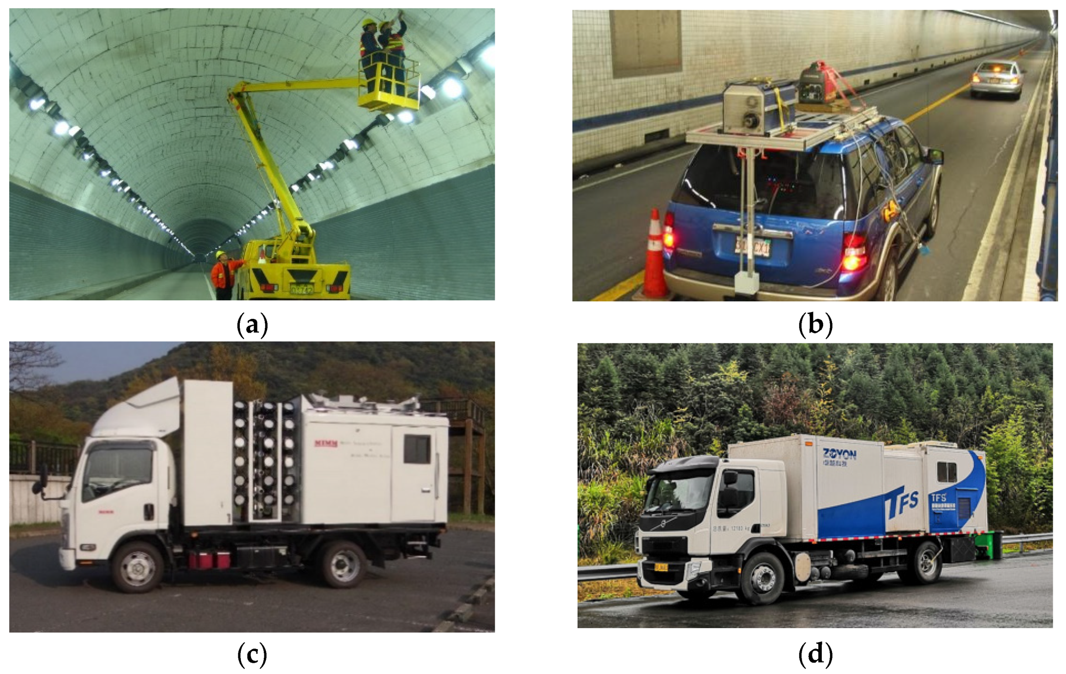
Typical tunnel structural-defect-identification methods are performed through visual inspections and non-destructive techniques, which usually detect all the exposed surfaces of structural elements at a close range, as shown in Figure 1a. Once the cracks are noted, they are classified as minor, moderate, or severe, which are the technical specifications for tunnel-maintenance purposes. All the noted cracks are then measured, and their locations are documented.

2.1. Tunnel Inspection Vehicles

Recently, tunnel inspection vehicles have been used to improve the efficiency of performing visual inspections [36,37], which mainly use various traveling sensors to detect the tunnel’s surface, and tunnel-lining disease is detected through image-processing or point cloud-processing methods. According to the different types of available sensors, rapid-inspection systems are divided into two categories: laser-scanning and calibrated laser/camera hybrids systems.

Laser scanners are used to collect target surface morphology information. They mainly scan the relevant spatial points with a certain resolution and create a 3D model or quantitative calculation to obtain the color and shape of the tunnel’s surface. Since the 1990s, laser techniques have been extensively used in the fields of object and surface-feature extraction methods and 3D reconstruction [38,39,40]. German SPACETEC TS3 (Figure 1b) was the first example of 3D-laser mobile tunnel-measuring equipment in the world, with a scanning frequency of 300 Hz, a panoramic measurement feature, a measuring speed of 4.5 km/h, and a crack-identification accuracy of 0.3 mm.

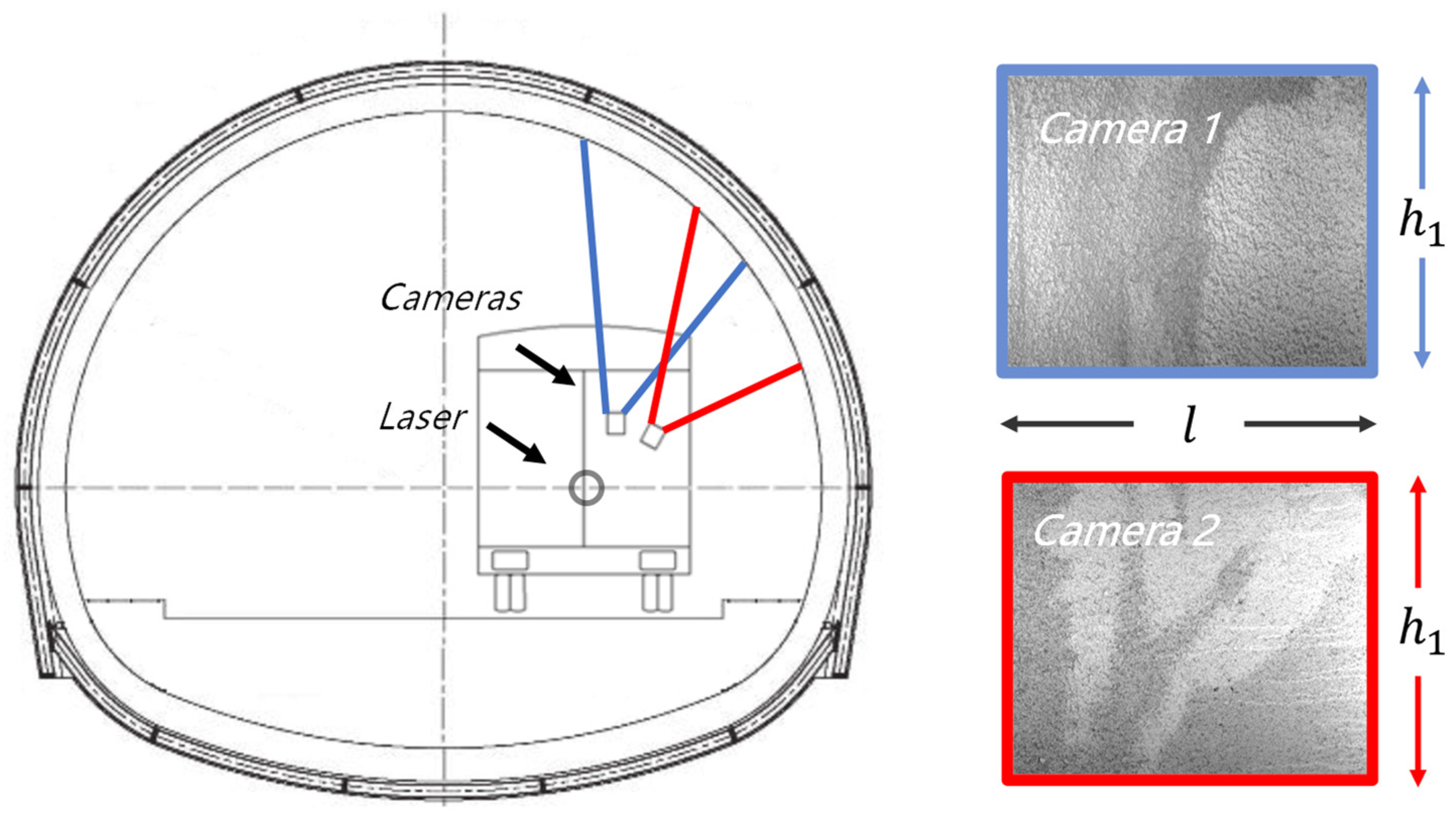
A typical hybrid inspection vehicle is Japan Keisokukensa MIMM-R (Figure 1c). The hybrid system simultaneously obtains tunnel wall images and point clouds using a laser. Laser-scanning systems obtain the shape of the tunnel-lining surface as 3D coordinates through laser measurements with a sampling rate and establish a concave–convex and deformation model of the concrete-lining surface. Multiple high-precision cameras collect images of the lining surface and stitch them together to form a layout map. The mileage positioning system records the distance between each measured section (the positioning points in the tunnel) and reference point. The image and laser synchronous positioning system determines the absolute position of the reference point to establish the appropriate position coordinates, and then completes the real-time measurements of the speed, displacement, and behavior of the tunnel-detection vehicle.

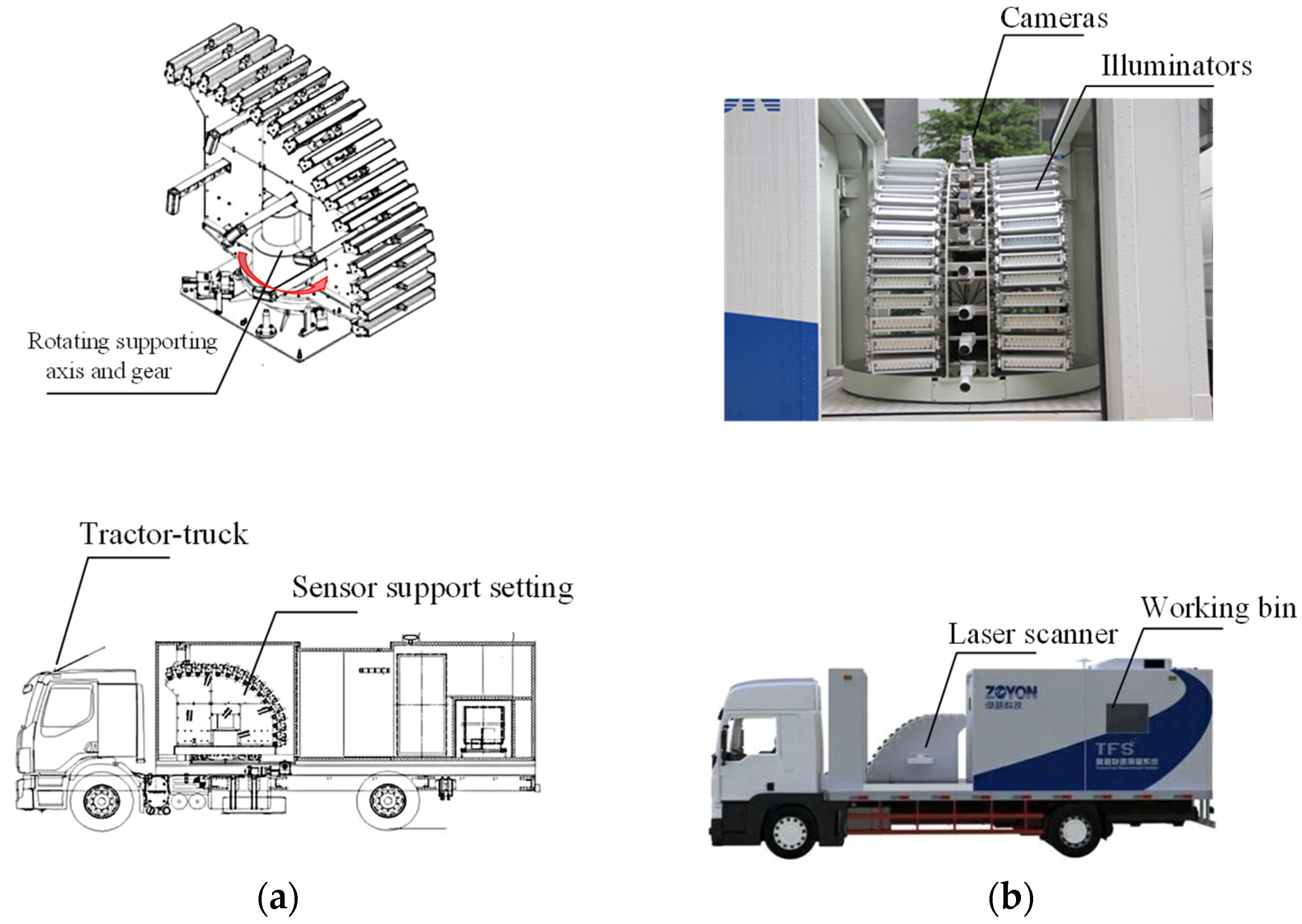
ZOYON-TFS (Figure 1d) was used in this study. Its measuring technique collects the necessary information for the tunnel-lining surface layout, including sequence images and tunnel contours. The former requires multiple cameras to perform continuous scans; the latter requires a laser scanner. All the sensors were set on the sensor support setting (Figure 2), which is located in the middle section of ZOYON-TFS. Cameras, laser scanners, and illuminators were also set to the sensor support setting. A rotating supporting axis and gear actualized the movement function with a servomotor drive system.

An area array camera was used to inspect the defects of the tunnel-lining surface. Multiple cameras were used at equal distances along the driving direction. Then, the coordinate transformation values obtained from each camera for the lining surface layout were used to preliminarily calculate the external parameters and working distance values. The trigger interval value should be lower than the horizontal field of view to avoid the occurrence of information loss.

To obtain the trade-off values for time, cost, and quality factors, a method based on two scans was employed by using the appropriate measuring units. Sensors collected information for one side of the tunnel-lining surface layout (the right or left sides of the tunnel), and the other side of the tunnel-lining surface layout was evaluated during a second journey by horizontally rotating the whole support setting.

2.2. Image-Range Stitching Method

Image-range stitching is an important component of automatic tunnel inspection systems; its function is to reconstruct images into presenting tunnel-lining surface layouts. It must solve the projected equation obtained from the camera measurement coordinate to the tunnel-lining surface layout coordinate system.

2.2.1. Tunnel-Lining Surface Layout Mapping

Tunnel panorama refers to the transformation of a 3D global coordinate system to a 2D coordinate layout through simple image mosaic technology [41,42], where the geometric distortion of images must be rectified prior to its application [43,44]. The configuration of a tunnel’s lining can be defined by geometric algebraic equations. The lining surface of a tunnel fitted by a multi-center curve (Figure 3a).

The lining surface in the 3D global Cartesian coordinate ($X$, $Y$, $Z$) is given by:

$$\left\{\begin{array}{c}{X}^2+Y^2=R^2\left(\beta \right)\\ 0\le Z\le L\end{array}\right.$$

(1)

where $L$ is the tunnel length, $R\left(\beta \right)$ is the tunnel radius, and $R\left(\beta \right)$ can be a constant for the circular lining. However, a highway tunnel’s lining is flatter, and its design is more complex. This manuscript proposes that simple laser-ranging technology rectifies the dynamic radius $R\left(\beta \right)$ and rotation angle $\beta$, and the primary radius $R$ was measured using a laser scanner.

For any point $P_1$ with a longitudinal distance $Z_1$ from the origin of the coordinate and rotation angle ${\beta }_1$ measured from the horizontal axis, the coordinates ($X_1$, $Y_1$, $Z_1$) of point $P_1$ can be presented as:

$$\left\{\begin{array}{c}{X}_1=R\left({\beta }_1\right)\times \cos \left({\beta }_1\right)\\ Y_1=R\left({\beta }_1\right)\times \sin \left({\beta }_1\right)\end{array}\right.$$

(2)

Figure 3b presents the layout of a tunnel-lining surface spread out from the tunnel wall image presented in Figure 3a. The points $a_i$, $b_i$, $c_i$, and $d_i$ in the layout correspond to points $A_i$, $B_i$, $C$, and $D_i$ in the 3D coordinate system, respectively. The 2D-image coordinates ($m_1$,$n_1$) for point $P_1$ can be determined via a coordinate transformation and are presented as:

$$\left\{\begin{array}{c}{m}_1=Z_1-Z_0\\ n_1={\int }_{\beta ={\beta }_0}^{\beta ={\beta }_1}\sqrt{{R\left(\beta \right)}^2+{R^{\prime }\left(\beta \right)}^2}d\beta \end{array}\right.$$

(3)

where the 3D global Cartesian coordinates of the tunnel-lining surface are transformed into the corresponding 2D surface layout. $Z_0$ is the initial distance of the tunnel layout and ${\beta }_0$ is the initial rotation angle.

2.2.2. Mapping the Image Center to the Tunnel-Lining Surface Layout

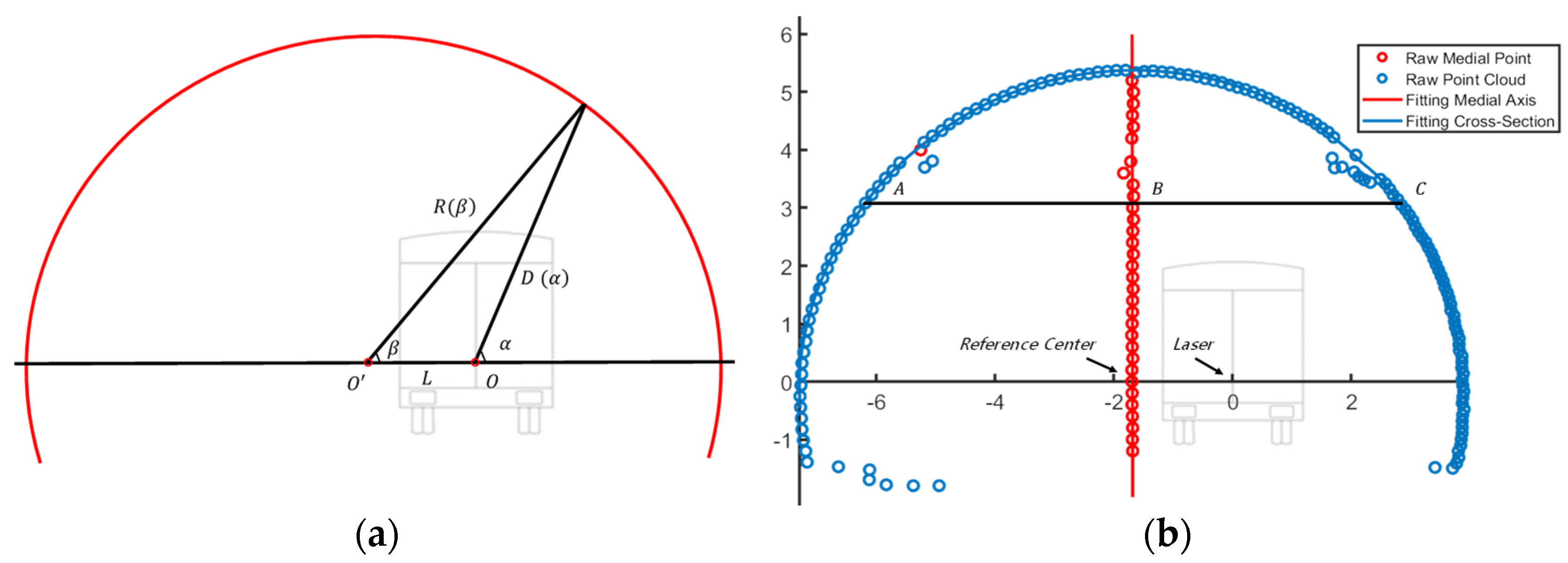
The measuring unit moves in one direction along the tunnel, with the laser scanner measuring the geometry of each section in the tunnel. The tunnel section is measured completely when the laser scanner rotates 360 degrees. Figure 4 presents the point cloud and measurement results. Figure 4a presents a diagram of the tunnel-section measurement, point $O$ is the coordinate origin of the measuring unit, and point $O^{\prime }$ is the reference center. The equations transform the 3D global Cartesian coordinates of the tunnel-lining surface into the corresponding 2D surface layout, with $O^{\prime }$ representing the origin in each section. The dynamic radius $R\left(\beta \right)$ and its rotation angle $\beta$ with $O^{\prime }$ as the origin were determined by the laser scanner. The laser scanner rotated 360 degrees by its center point $O$, ranging between every fixed angle. The angle sensor measured the rotation angle of each point; the main controller received the range $D\left(\alpha \right)$ and angle $\alpha$ measurements, as presented in Figure 4a. The blue point presented in Figure 4b represents the raw point cloud of a single section. The laser scanner rotated 360 degrees to collect 540 points, the bottom 90 degree points were eliminated, and the top 270 degree points were retained. The eliminated point cloud represents the pavement; the retained point cloud values represent the tunnel’s main structure and auxiliary equipment.

The point-cloud processing stage represented in this study consisted of the following steps. Firstly, the maximum and minimum values in horizontal-axis direction (points $A$ and $C$ in Figure 4b) were calculated by the tunnel design clearance height, which is usually approximately 3 m. Point $B$ presented in Figure 4b is the midpoint of points $A$ and $C$. Secondly, all the midpoints (red point in Figure 4b) were fitted to the central axis of the tunnel (red line in Figure 4b) by RANSAC or the least-squares method [45]. The intersection of the tunnel’s central and $x$-axes (point $O^{\prime }$ in Figure 4b) was defined as the reference center of the tunnel section. Then, the distance $R_i$ from the point cloud values for a 360 degree rotation of the laser scanner to the reference center are calculated using the following formula:

$$R_i=\sqrt{L^2+{D_i}^2+2L{D}_i\times \cos \left({\alpha }_i\right)}$$

(4)

where $L$ is the distance between points $O$ and $O^{\prime }$, and $i$ represents all the retained raw point-cloud values, $i$ = 1, 2, 3, …. The angle ${\beta }_i$ obtained from the raw point-cloud values to the reference center are calculated by:

$${\beta }_i=\arcsin \left[\left(\frac{D_i}{R_i}\right)\ast \sin \left({\alpha }_i\right)\right]$$

(5)

Figure 5 shows the transformations obtained from each camera, where the distance $R_i$ and angle ${\beta }_i$ were filtered using the median-filtering method and the curve was fitted as a function $R\left(\beta \right)$, which was the clean distance of the main structure relative to the tunnel center (red line in Figure 5b). Function $R\left(\beta \right)$ was the first variable in the equations used to transform the 3D global Cartesian coordinates of the tunnel-lining surface into the corresponding 2D surface layout. The second variable was the optical axis angle ${\beta }_1$ of each camera, which was determined by a static calibration. The image center $P$ was mapped onto the tunnel-lining surface layout with these variables.

2.2.3. Mapping Image Space to the Tunnel-Lining Surface Layout

The area array camera used in this work was triggered by the encoder at equal intervals. The image sequences obtained by each single camera (shown in Figure 5a) were continuous, with overlaps and geometric distortions being caused by the tunnel’s surface, which was not flat.

The tunnel-lining surface was nonlinearly relative to the camera’s field of view, resulting in production of a geometrically distorted trapezoid shape. Figure 5 shows the coordinate transformation of a camera with a field of view ranging from points $P_A$ to $P_B$ on the tunnel-lining surface. The coordinate transformation in tunnel-lining surface layout and the length from point $P$ to the origin $O$ satisfies the following equation:

$$\frac{l}{L}=\frac{l_A}{L_A}=\frac{l_B}{L_B}$$

(6)

where $L_A$ and $L_B$ represent the distance from point $P_A$ and $P_B$ to origin $O$; $l_A$ and $l_B$ are the width of point $P_A$ and $P_B$ in the tunnel-lining surface layout.

The resampled and real-time image stitching require a balance between the stitching performance and efficiency. A possible compromise is the proposition that the lower distortion outcome can be ignored, while the greater distortion outcome needs to be resampled following the coordinate transformation step in the tunnel-lining surface layout. The distortion is proportional to the maximum difference of the width $∆l$. The images were resampled, while $∆l$ is larger than the threshold value:

$$∆l=\mathit{max}\left(l_A,\dots ,l,\dots ,l_B\right)-min\left(l_A,\dots ,l,\dots ,l_B\right)$$

(7)

Combined with the Equations (6) and (7), the maximum difference of the tunnel-lining surface values shows that the origin is greater than the threshold value, and the images were resampled.

$${\beta }_i=\arcsin \left[\left(\frac{D_i}{R_i}\right)\times \sin \left({\alpha }_i\right)\right]$$

(8)

Once the two adjacent images were registered, the overlapping regions were merged using image-fusion methods to form a composite image. There are several image-stitching techniques used in the research, such as alpha blending [46,47] and gradient domain methods [48,49]. Considering that the images obtained by different CCDs usually present significant differences in their gray-scale values, Poisson blending [50,51] was used, which naturally pastes two images together because the human visual system is more sensitive to gray-scale contrast than intensity.

2.3. Semantic-Based Crack-Detection

Computer vision is based on an extensive set of diverse tasks combined to achieve highly sophisticated applications. Typical computer vision tasks include [15] image classification (Figure 6a), localization, object detection (Figure 6b), segmentation (Figure 6c), and object tracking.

The above methods share similarities and are regarded as labeling processes for crack detection. Classification tasks involve labeling images, detection tasks involve labeling blocks, and segmentation tasks involve labeling pixels. The correct label, also known as the ground truth, conforms to human cognition. It necessitates a translation between two distinct forms of information: vision and labels. However, when labels are converted into images, information about the color, texture, and other features of cracks is lost.

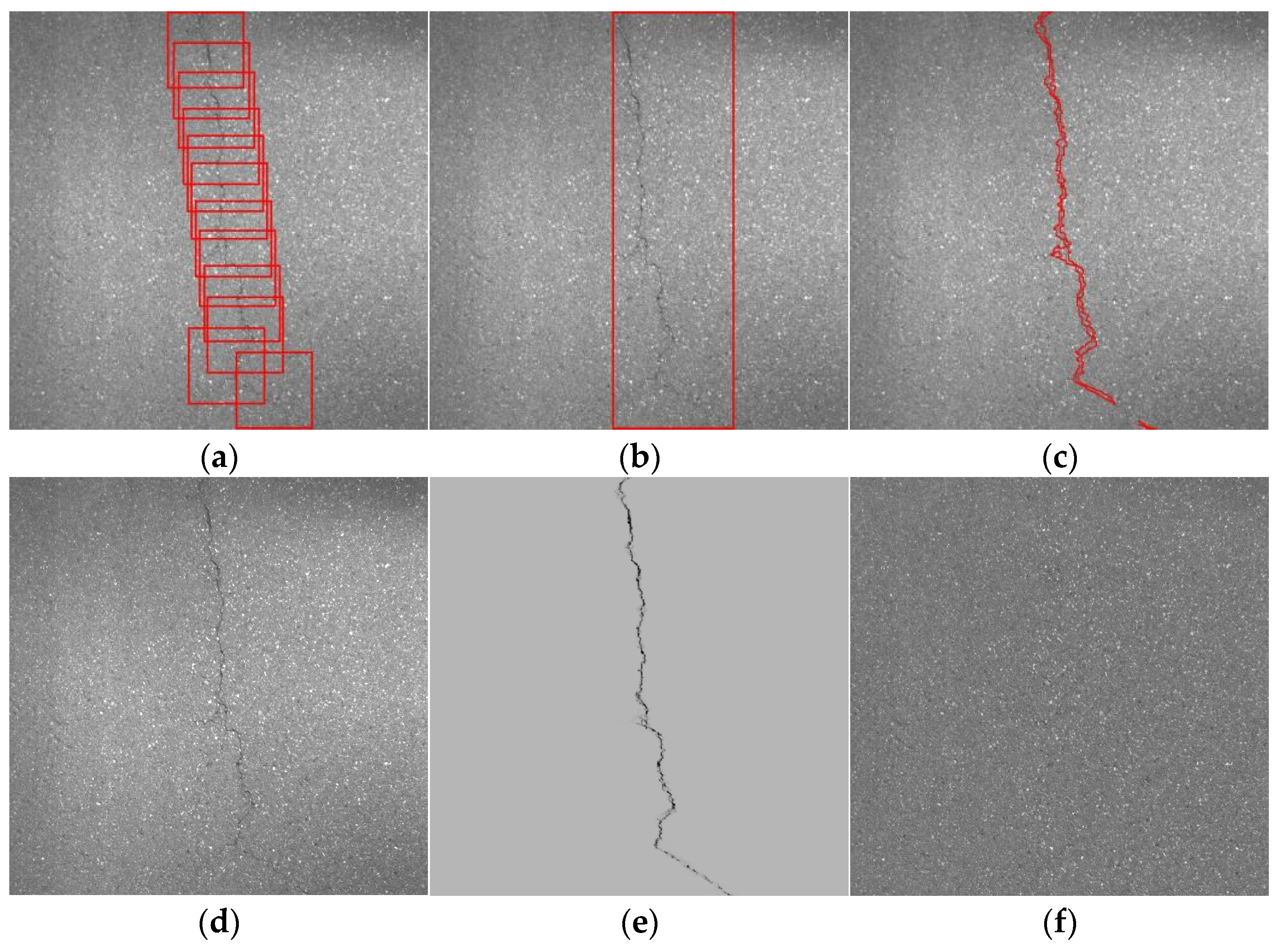
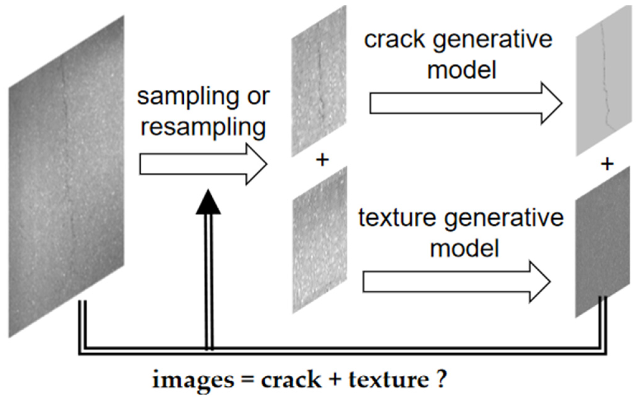
To address this issue, an image generation model was employed as a container. The crack detection task was reframed as a semantic separation problem. The objective was to segment each semantic component into distinct semantic containers (Figure 6d–f). This approach operates as an intelligent filter, superior to any other labeling technique. While Fourier filters separate images into high-frequency and low-frequency components, this method separates images into crack components and texture components (Figure 7).

The method is simply described as the following steps: first, the pixels are randomly labeled with cracks and textures; second, the pixels labeled as cracks and labeled as textures are respectively assigned to the crack generation and texture generation. You can use any method or model you like; third, comparing the original image with its generated results. If they are not consistent, it is most likely due to incorrect labeling and require resampling (usually resampling the region with the greatest difference). Label based crack detection is usually targeted to achieve 100% pixels accuracy and precision. In comparison, this method only requires labels to be accurate enough to implement cracks and/or texture components to image generation container matching.

2.3.1. The Preprocessing Step

Tunnel-lining surface images present rich environmental information, and precise texture extraction is a key factor used to reduce the uneven brightness in the images. According to the Retinex theory [52], an image is determined by two factors: the reflection property of the object itself and the light intensity around the object. The illumination intensity determines the dynamic range of all pixels in the original image, and the inherent attribute (color) of the original image is determined by the reflection coefficient of the object itself. Therefore, this method divides an image $S(x,y)$ into two different images, reflection $R(x,y)$ and lightness $L(x,y)$, and then removes the influence of illumination and retains the inherent properties of the object:

$$S(x,y)=R\left(x,y\right)\times L\left(x,y\right)$$

(9)

where the effective illumination $L(x,y)$ is represented by the alignment of the penumbra strip (Figure 8) [53].

To achieve an effective evaluation of the shadows in the image, it was necessary to eliminate the influence of variable penumbra areas. Gaussian filtering or a similar filtering algorithm presents the general intensity distribution of the illumination change with some minor errors remaining. It was assumed that the intensity change trend was similar after intense outlier filtering; however, differences only appeared in the noise level (such as background texture) and presented some minor errors. A small-scale optimization was needed to solve the problem of consistency. For each image sub-block (strength profile), the alignment process shifted the center of the column vertically, and then stretched the column around its center by moving both its ends. The fine alignment parameters of each column are estimated by minimizing the following energy function $E_a$:

$$L_n=\Gamma \left(A_s,A_k,L_o\right)$$

(10)

$$E_a=MSE\left(L_n-L_a\right)$$

(11)

where $A_s$ and $A_k$ are the stretching and center displacement values in the fine scale alignment, $L_o$ is the proportion of the original column, $L_a$ is the alignment reference (it is the average proportion value for all effective columns), $L_n$ is the alignment expansion, $\Gamma$ is the function of alignment $L_o$ according to the estimated alignment parameters, and $MSE$ is the function of calculating the mean square error value. The sequential quadratic programming algorithm was used to solve the minimization problem [54].

2.3.2. Random Sampling with Gray-Scale Sparsity Prior Function

The crack pixels are sparse signals and can be approximately and efficiently reconstructed using a small number of random sampling measurements [55,56]. This process is known as compressed/compressive sensing (CS). The compressed-sensing framework and supporting theory prove that, when the sampling rate is lower than the critical sampling rate, the original ill-posed signal-recovery and -reconstruction problem can achieve perfect signal-recovery results with the help of additional sparsity prior functions.

The random sampling with gray-scale sparsity prior functions (shown in Algorithm 1) used in this work were as follows. Each time, it randomly selected several pixels and retained a certain proportion of pixels with lower gray-scale value. This process was repeated until the selected pixels provided adequate information for crack-detection purposes. Here, the condition was simply defined as the crack-detection stage, requiring 1/64 of the down sampling stage for sensing the appropriate values.

Algorithm 1. Random Sampling with Sparsity Prior Algorithm

Symbols used in the algorithm:

x: Pixel being Processed

y: Pixel Sampled

r: Random Sampling Ratio

R(x, amount): Random amount of Pixels in x

S(x, percentage): Select the darkest pixel

while length(y) < r × length(x)

x0 = R (x, amount);

y ∈ S(x0, percentage);

end while

The crack pixels were darker than the background [57,58] and independent in the gray-level distribution. In other words, the pixels containing rich information usually met the abovementioned conditions. Usually, these information-rich pixels ranged from 0% to 30%, which varied with the amount of information contained in the image. Meanwhile, these informative pixels were spatially continuous, connected, and presented consistent features and high redundancy results [59,60,61]. These conditions showed that cracks can be reconstructed using a reduced number of data/measurements than what is usually considered necessary in the literature.

2.3.3. Crack Generator

Variational Auto-Encoder (VAE) [62] was used for crack-generation purposes. The framework for VAE is presented in Figure 9. VAE introduces the hidden variable $z$ in the model to maximize the probability $p_{\theta }(x)=\int p_{\theta }(z)p_{\theta }(x|z)dz$ of the desired distribution $p(x)$ of gray values. In Figure 9, the encoder is a variation distribution model, $z~q_{\varphi }(z|x)$; the decoder is a conditional distribution model, $x~p_{\theta }(x|z)$; and $p\left(x\right)$ is a prior value for the hidden variables, $p\left(x\right)$. Compared with Auto-Encoder (AE), the variable $z$ in VAE was deterministic and there was no prior $p\left(z\right)$ value. The VAE framework is a stochastic version of AE; hidden variable $z$ is a random node. To solve this problem, reparameterization was needed.

To solve for the gradient of expectation with random variables, the Monte Carlo estimator $E_{z~q_{\varphi }(z|x)}$ was used:

$$\begin{array}{cc}{\mathsf{\nabla }}_{\varphi }{E}_{z~q_{\varphi }(z|x)}[f(z)]& =E_{z~q_{\varphi }(z|x)}[f(z){\mathsf{\nabla }}_{\varphi }ln{q}_{\varphi }(z|x)]\\ & \approx \frac{1}{N}{\sum }_{i=1}^{N}f(z_i){\mathsf{\nabla }}_{\varphi }ln{q}_{\varphi }(z_i|x)\end{array}$$

(12)

where the observed variable is $x$, and the hidden variable is $z$. $q_{\varphi }(z|x)$ is the variation distribution of the hidden variable $z$ and $\varphi$ is its antecedent node.

Reparameterization changes $z$ from a random variable to a deterministic variable, $z~q_{\varphi }(z|x)$ becomes $z=g_{\varphi }(x,\mathsf{ϵ})$, and the gradient is

$${\mathsf{\nabla }}_{\varphi }{E}_{z~q_{\varphi }(z|x)}[f(z)]\approx \frac{1}{N}{\sum }_{i=1}^N{\frac{\partial f}{\partial g}\frac{\partial g}{\partial \varphi }|}_{g=g_{\varphi }(x,{\mathsf{ϵ}}_i)}$$

(13)

where the randomness is transferred to variable ϵ, at which point $z$ becomes a deterministic node and the gradient can be passed through it to its antecedent node $\varphi$.

2.3.4. Lining Generator

Image inpainting fills the missing part of the image with the content similarity present in the image or the semantic and texture information learned from large-scale data. Exemplar-based image inpainting [63] is the most classical method. It notes that exemplar-based texture synthesis contains the essential process required to replicate both texture and structure; the success of structure propagation, however, is highly dependent on the order in which the filling proceeds. We proposed a best-first algorithm in which the confidence in the synthesized pixel values was propagated in a manner similar to the propagation of information in the inpainting method.

The algorithm proceeded as follows, calculating the priority of the point $P$ to be patched. The priority $P\left(p\right)$ is composed of two parts:

$$P\left(p\right)=C\left(p\right)D\left(p\right)$$

(14)

where $C\left(p\right)$ indicates the reliability of the point and $D\left(p\right)$ is a term calculated based on the data surrounding the region to be patched. $C\left(p\right)$ can be considered as the confidence level of the points surrounding $p$, with the aim of preferentially filling those regions surrounded by more known points. It is calculated as follows:

$$C(p)=\frac{{\sum }_{q\in {\Psi }_p}C\left(q\right)}{\left|{\Psi }_p\right|}$$

(15)

where the marker ${\Psi }_p$ is the area to be repaired, with $p$ as the center block. $D\left(p\right)$ is used to fill the points with stronger grain structures in order of priority, which is calculated as follows:

$$D(p)=\frac{|▽I_p^{∟}·n_p|}{\alpha }$$

(16)

The normal direction of the contour $n_p$ to be filled is obtained at point $p$; $▽I_p^{∟}$ means that its gradient direction is rotated by 90 degrees, so that the point $p$ with stronger structural features can be obtained. ${\Psi }_p$ is the area to be repaired with $p$ as the center block. We find a block with the highest similarity ${\Psi }_q$ in the image and fill it with ${\Psi }_p$. Then, update $C\left(p\right)$, $C\left(p\right)$ = $C\left(q^{\prime }\right)$. We repeat the abovementioned process until all the regions are filled in.

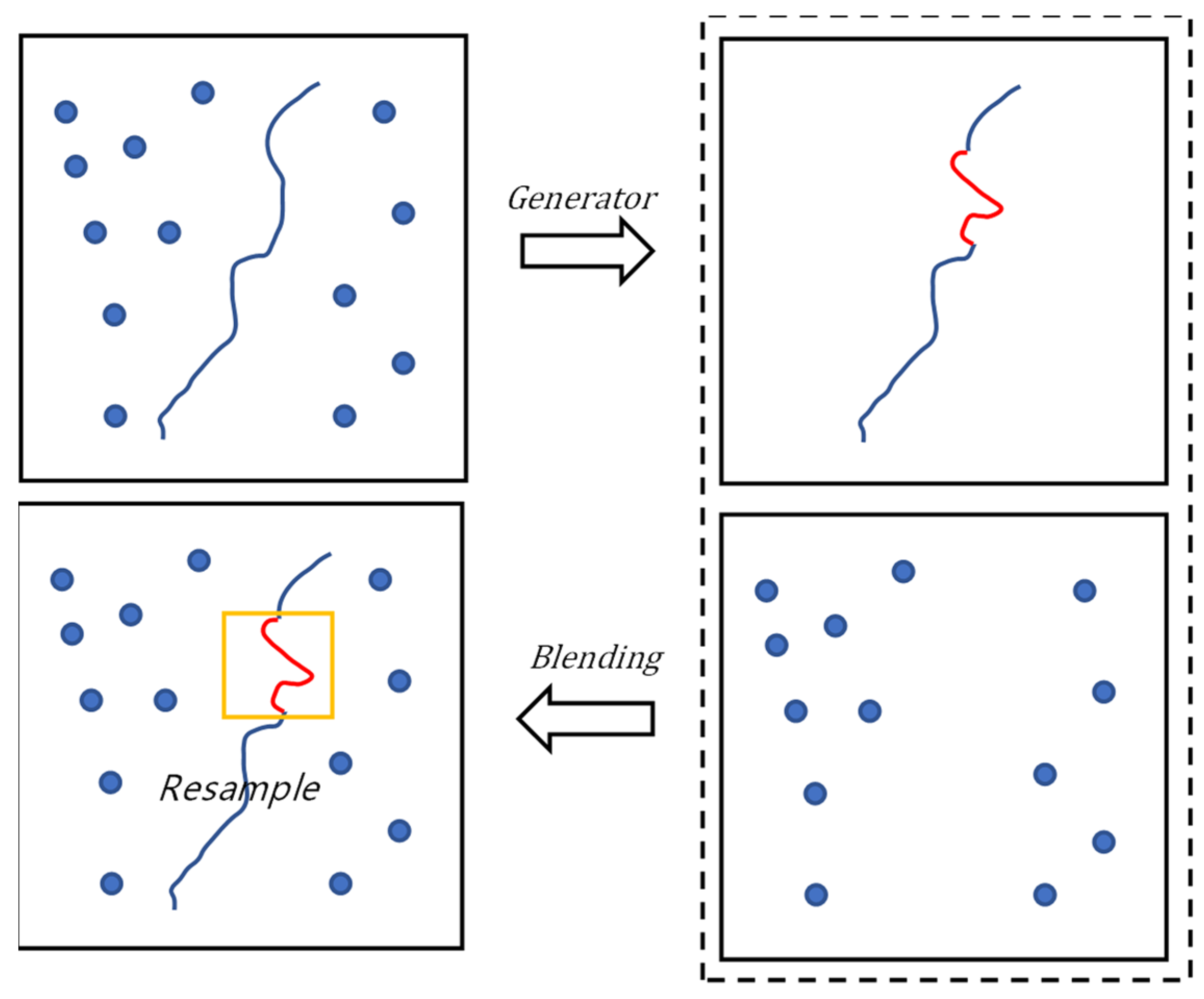
2.3.5. Region Resample

Suppose that $x$ is the crack image and the value to be solved. $\rho$ is the observation matrix, which corresponds to the sampling process and is known. It projects the high-dimensional signal $x$ into the low-dimensional space. Then the sampling result $y$ is also known and satisfies the equation

$$y=\rho x$$

(17)

$\mu$ is the semantic matrix, which is also known for the crack-generation process.

$$x=\mu y$$

(18)

The observation and semantic matrices satisfy the function $\mu ={\rho }^{-1}$. Traditional generation algorithms can construct the semantic matrix by tuning the reference, and data-driven generation algorithms can construct the semantic matrix by training.

Due to the error $\delta \rho$ between the observation matrix used for random sampling and the observation matrix used to generate the semantic matrix, the actual acquisition result is $y+\delta y$:

$$y+\delta y=(\rho +\delta \rho )x$$

(19)

where $\delta y$ is the value to be corrected. At this point, a crack with bias $x+\delta x$ is generated.

$$x+\delta x=\mu (y+\delta y)$$

(20)

$\delta x$ is the known quantity. It can be obtained by comparing the image to be detected with the semantic generated image, that is, the generated crack and pavement images are fused, and the pixel difference between the fused image and the image to be detected is $\delta x$.

For this problem, the region resample process is presented in Figure 10, where the image to be detected is sampled, cognitively generated, and the crack and pavement images are obtained. The crack and pavement images are fused and compared with the image to be detected. Resampling is then performed for images presenting large pixel differences. The image to be detected is $I\left(p\right)$ and the generated crack and pavement images are fused into a new image based on Poisson’s fusion method as $G\left(p\right)$. The sampling point is $q$ and ${\Pi }_p$ is the attachment region centered at $p$. Then, the region close to $p$, the pixel difference $\delta x$ between the image to be detected, and the fused image satisfies the equation.

$$\delta x=\overline{({\Pi }_{I\left(p\right)}-{\Pi }_{G\left(p\right)})}$$

(21)

3. Results and Discussion

3.1. Sensor and Calibration

Figure 11 presents the principle of the multi-camera imaging method; each camera is responsible for a sector and overlaps with each adjacent area, covering a range of approximately 90 degrees. Generally, the cross-section of a highway tunnel adopts single- or multi-center circles and its height value changes minimally; therefore, it is necessary to select and install lenses with different focal lengths or cameras with different resolutions to ensure consistent accuracy in tunnel-lining surface image mapping. The images captured by the camera each time are reconstructed and projected onto the tunnel-lining surface layout. The reconstructed images have the same width $l$, and the height $h_i$ is calculated by the imaging principle.

The system employs an 8-bit monochrome CMOS sensor with a resolution of 2752 × 2208, utilizing dynamic ISO and exposure. It corresponds to a laser scanner with a resolution of 0.5°, a spot size of 8 mm, a resolution of 10 mm, and a typical error of 30 mm. The tunnel inspection vehicle collects data at a speed of 80 km/h with triggered equidistant wheel encoder. Each frame contains 16 camera images and point cloud around this cross-section. The encoder is triggered once every 0.3 m in the experiment, ensuring extensive image overlap for traditional image stitching. At ordinary times, the proposed method generally operates with 20 frames or less. The working distance and the field of view of 16 cameras are different, so the resolution and overlap are not consistent.

Sensor installation and calibration are important to ensure good data-fusion performance and quality control [64]. Sensor installation requires considerable manual post-installation work before the center line of images corresponds to the same line in tunnel-lining surfaces. Continuous adjustments are needed to ensure that the front and back positions of each camera are aligned with and are parallel to the cross-section profiles of the camera and object. The cameras should be calibrated following their installation. Calibration is generally divided into two steps: the calibration of each sensor’s own parameter and installation, and the joint calibration of multiple sensors. The calibration of each sensor’s own parameter ensures its accuracy, and the joint calibration of multiple sensors accurately mosaics the calculation results. The calibration of each camera’s own parameter is performed using the Zhang calibration method [65,66].

To achieve the complete calibration of each camera, a dozen different images of the same calibration checkerboard were used to calibrate the internal parameters. Figure 12a shows the calibration site for the joint calibration of multiple sensors. It is a half-tunnel model of an equal size (the orange steel frame in Figure 12a); the inner side is the calibration board shown in Figure 12b. The calibration board has two purposes: camera installation and positioning, and camera resolution testing. Figure 12b presents the calibration board captured by the camera; the image center line (red line in Figure 12b) is used as a reference of collinear points.

The camera installation setup was as follows: first, each camera was installed using a theoretical value with a field-of-view height of about 750 mm. Secondly, we adjusted the cameras until the actual field of view for adjacent image overlapping was 50 ~ 100 mm. Then, we adjusted the cameras until the image center line coincided with the reference of collinear points (red line in Figure 12b). Lastly, we calibrated the installation parameters of the sensors; all sensors were fixed and not adjusted further.

The laser scanner was applied to the same calibration site presented in Figure 12. The laser scanner was installed at the focal point of the optical axis extension line. To achieve better measurements, the optical axis of all the cameras should be in the same space plane, and the laser-scanning plane should be positioned parallel to this plane. The conditional random field (CRF) model [67] was used to calibrate the cameras and laser scanner. The laser scanner (point $O$ in Figure 12c) was used as the reference of the multi-sensors system; the coordinate value of the lining contour relative to the laser was obtained by processing point clouds. The cameras (point $C$ in Figure 12c) were calibrated and the optical axis satisfies the following equation:

$$Y=\left(X-X_0\right)\times \tan \left(\alpha \right)+Y_0$$

(22)

where $\left(X_0,{ Y}_0\right)$ is the coordinate value relative to the laser and $\alpha$ is the angle of the optical axis offset.

The imaging area of the camera was a rectangular area centered on the focal point (point $I$ in Figure 12c) of the optical axis and the surface plane of lining. The working distance of the camera $d$ is achieved by the camera coordinate and focal point:

$$d=\sqrt{b^2+h^2-2bh\times \cos \left(\alpha -\beta \right)}$$

(23)

where $\beta$ is the angle of point $I$ measured by the laser, $h$ is the distance of point $I$ measured by the laser, and $b$ is the distance between the laser and camera, $b=\sqrt{{X_0}^2+{Y_0}^2}$.

A series of measurement points on the lining section were collected by the laser, and the one closest to the optical axis was point $I$. The imaging area of the camera in the transverse section is approximately:

$$L=2d/\tan \theta$$

(24)

where $2\theta$ is the field of view of the camera.

The half-section of the tunnel-lining surface was divided into 15 equal segments based on its geometric dimension, and the imaging areas of the cameras were about $L$ = 0.75 m for each camera. The installation angle of the optical axis offset ${\alpha }_i$ of camera $i$; this angle was also the center point of the imaging area of the cameras, which is fixed at:

$${\alpha }_i={\beta }_i+\arccos \left(\frac{{b_i}^2+{h_i}^2-{d_i}^2}{2b_i{h}_i}\right)$$

(25)

where $b_i$ is the distance between the laser and camera $i$, $d_i$ is the distance between the focal point and camera $i$, $h_i$ is the distance between the focal point and laser, and ${\beta }_i$ is the angle between the focal point and camera $i$.

As

Table 1. Camera parameters.

Number	Focal Length	Optical Axis Angle(${\mathit{\beta }}_{\mathit{i}}$)	Installation Distance(${\mathit{b}}_{\mathit{i}}$)	Working Distance (di)	View Field of Camera		Pixel Resolution
					Width	High
1	35 mm	86.6°	1122 mm	2658 mm	950 mm	762 mm	0.23 mm
2	35 mm	81.3°	1115 mm	2518 mm	900 mm	722 mm	0.22 mm
3	35 mm	73.3°	1106 mm	2546 mm	910 mm	730 mm	0.22 mm
4	35 mm	66.7°	1102 mm	2602 mm	930 mm	746 mm	0.23 mm
5	35 mm	60.1°	1119 mm	2770 mm	990 mm	794 mm	0.24 mm
6	35 mm	53.5°	1143 mm	2966 mm	1060 mm	850 mm	0.26 mm
7	35 mm	46.6°	1185 mm	3273 mm	1170 mm	939 mm	0.28 mm
8	50 mm	39.8°	1237 mm	3477 mm	870 mm	698 mm	0.21 mm
9	50 mm	33.5°	1292 mm	3877 mm	970 mm	778 mm	0.24 mm
10	50 mm	26.9°	1356 mm	4396 mm	1100 mm	882 mm	0.27 mm
11	50 mm	20.2°	1411 mm	4836 mm	1210 mm	970 mm	0.29 mm
12	75 mm	13.1°	1468 mm	4915 mm	820 mm	658 mm	0.20 mm
13	75 mm	7.5°	1524 mm	5836 mm	970 mm	778 mm	0.24 mm
14	75 mm	0.3°	1549 mm	6475 mm	1080 mm	866 mm	0.26 mm
15	75 mm	-7.0°	1526 mm	5875 mm	980 mm	786 mm	0.24 mm

shows, 15 cameras (Nos. 1 to 15) were used in this study, with the optical axis angles ranging from -7.0 to 86.6 degrees. Three different focal lengths, 35, 50, and 75 mm, were selected. The camera with a shorter working distance had a shorter focal length, and the camera with a longer working distance had a longer focal length.

3.2. Result of Image Stitching

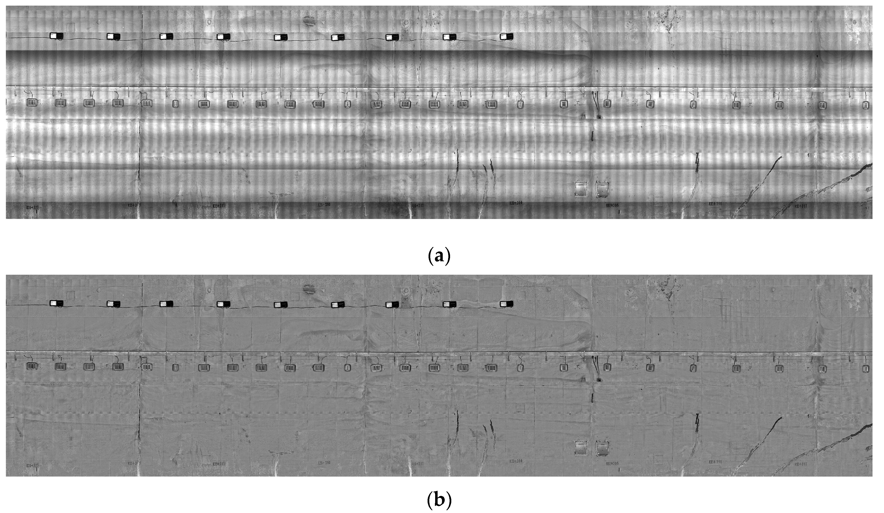
Figure 13 presents the layout of a tunnel lining, which combines 200 images taken by 16 cameras. Figure 13a presents the direct pixel mapping of image-range stitching and Figure 13b presents the mapping of the pre-processed images.

Here, image-range stitching was compared with AutoStitch [68], which is the most classic and widely used stitching algorithm in the research. AutoStitch uses SIFT features to match feature points, then uses the bundle adjustment process to calculate the image coordinate transformation parameters (similar to Homography [69]), and finally uses multi-band blending to obtain the final stitching map. The algorithm (shown in Algorithm 2) flow is presented as follows.

Algorithm 2. Automatic Panorama Stitching

Input: n unordered images

Extract SIFT features from all n images overlapping, overlapping is manually annotated

II: Find k nearest-neighbors for each feature using a k-d tree

III: For each overlap:

(i) Select m candidate matching images that have the most feature matches

(ii) Find geometrically consistent feature matches using RANSAC to solve for the homography between pairs of overlapping values

(iii) Verify overlapping matches using a probabilistic model

Output: Panoramic images

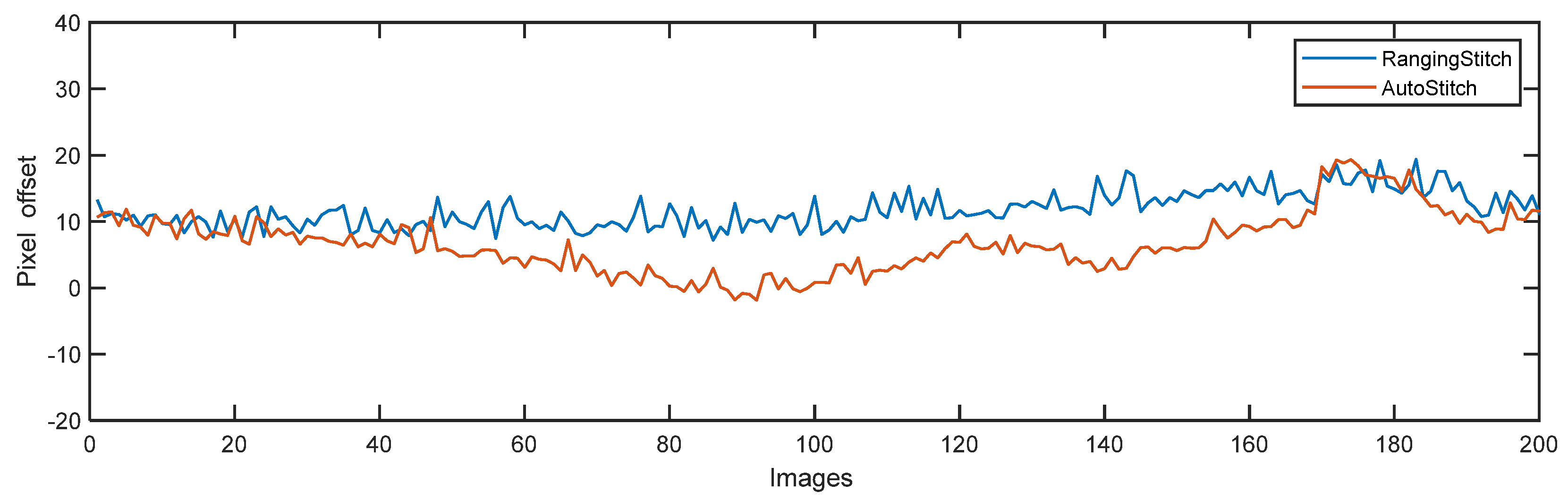
The overlapping of each image was roughly stitched manually (pixel offset = 0) and then stitched with ranging stitch and AutoStitch. The overlap area (the largest area with the clearest image) between cameras Nos. 10 and 11 was selected and the results are presented in Figure 14. Compared to AutoStitch, there was an error of 5.4689 pixels (standard deviation) in the ranged stitch image, leading to the misalignment of the image structure of typical targets, such as cracks and cables. This was the result of a range of factors, including sensor vibrations, calibration errors, and model errors.

The accuracy of image feature point-based (e.g., SIFT and ORB features) image-stitching methods heavily rely on the detection quality of feature points, and often fail in scenes with conditions of low texture, low lighting, repeated textures, or repeated structures. This is one of the difficulties faced by tunnel-lining image stitching. Although image feature points can be used as a reliable stitching reference in the case of pre-defined overlapping areas, image feature point-based image-stitching methods tend to fail when the overlapping area is uncertain. This is more common in some non-standard-sized tunnels.

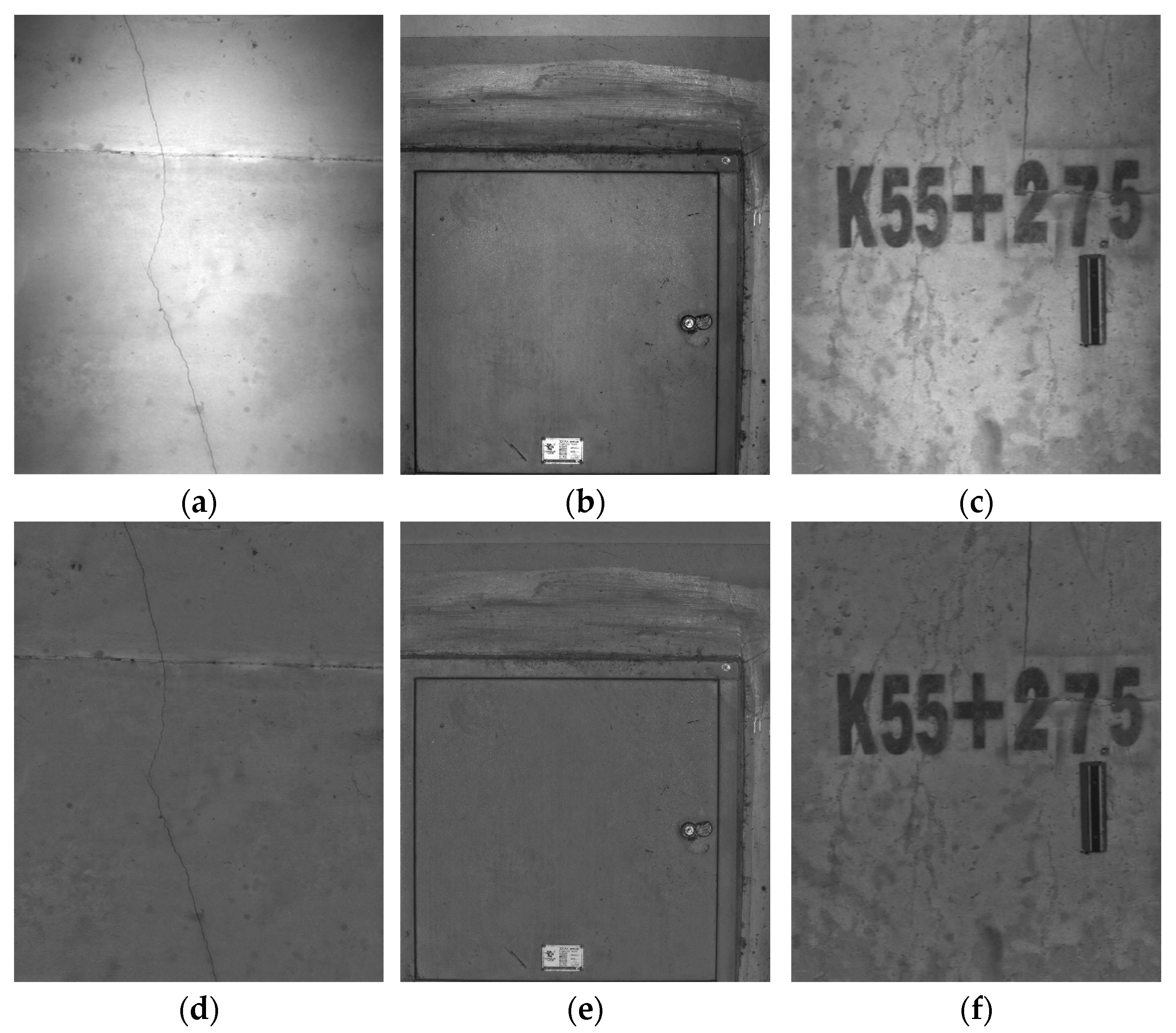
3.3. Result of Crack Detection

Figure 15 shows the image before and after the preprocessing stage. The quality of the original road image captured by CCD or COMS cameras depended on the appropriate exposure time and sensor sensitivity/ISO. When the camera works normally, the brightness of the image is moderate and the details of the image are rich; in the over/under exposure scenarios, the image is too bright and/or dark, loses a lot of necessary details, and produces a high amount of image noise. The textured plane of the image stripped by the abovementioned algorithm also showed that the region contained almost no texture information and there was considerable noise. These exposed areas should be detected and marked during the preprocessing stage and not be selected for feature point-matching or crack-detection methods. Any pixel with a gray level that was either too bright (higher than 225) or too dark (lower than 30) and with a local standard deviation value less than 1.8 should be regarded as an abnormal pixel. The lining texture image was divided into 64 × 64 regions. If more than 50% of the pixels in the region were abnormal, the region was marked as abnormal.

Figure 16 is the result of a semantic-based crack-detection method. The crack generator was observed as a filter that could only pass the crack semantics, while the lining generator was observed as a generator that could only pass through the lining component. The random sampling and region resample processes ensured that the information of the image was decomposed orthogonally, which must be built on the premise that cracks and textures are not dependent on each other.

Once the user is aware of the object, a more conceptual task appears: object-naming. This is where the semantic gap plays a greater role in the process. A semantic gap is usually defined in the literature as the difference between a user’s understanding of objects in images and the computer’s interpretation of these objects [59]. This semantic process does not concern pixel accuracy; two completely different diagrams can provide the same semantic details. This results in the “semantic gap” between the “semantic similarity” understood by people and the “visual similarity” understood by computers [60]. The semantic gap is a challenge for crack-detection algorithms in passive feature-matching-based methods.

Traditionally, the algorithm is taught to differentiate between cracks and non-cracks, with the “ground truth” being observed as a conceptual term relative to the knowledge of truth [61]. Quantitative metrics, such as precision, accuracy, and F1-score are used to describe the achievement rate of the “ground truth” for a specific task. Typically, algorithms with high precision and accuracy results are considered superior.

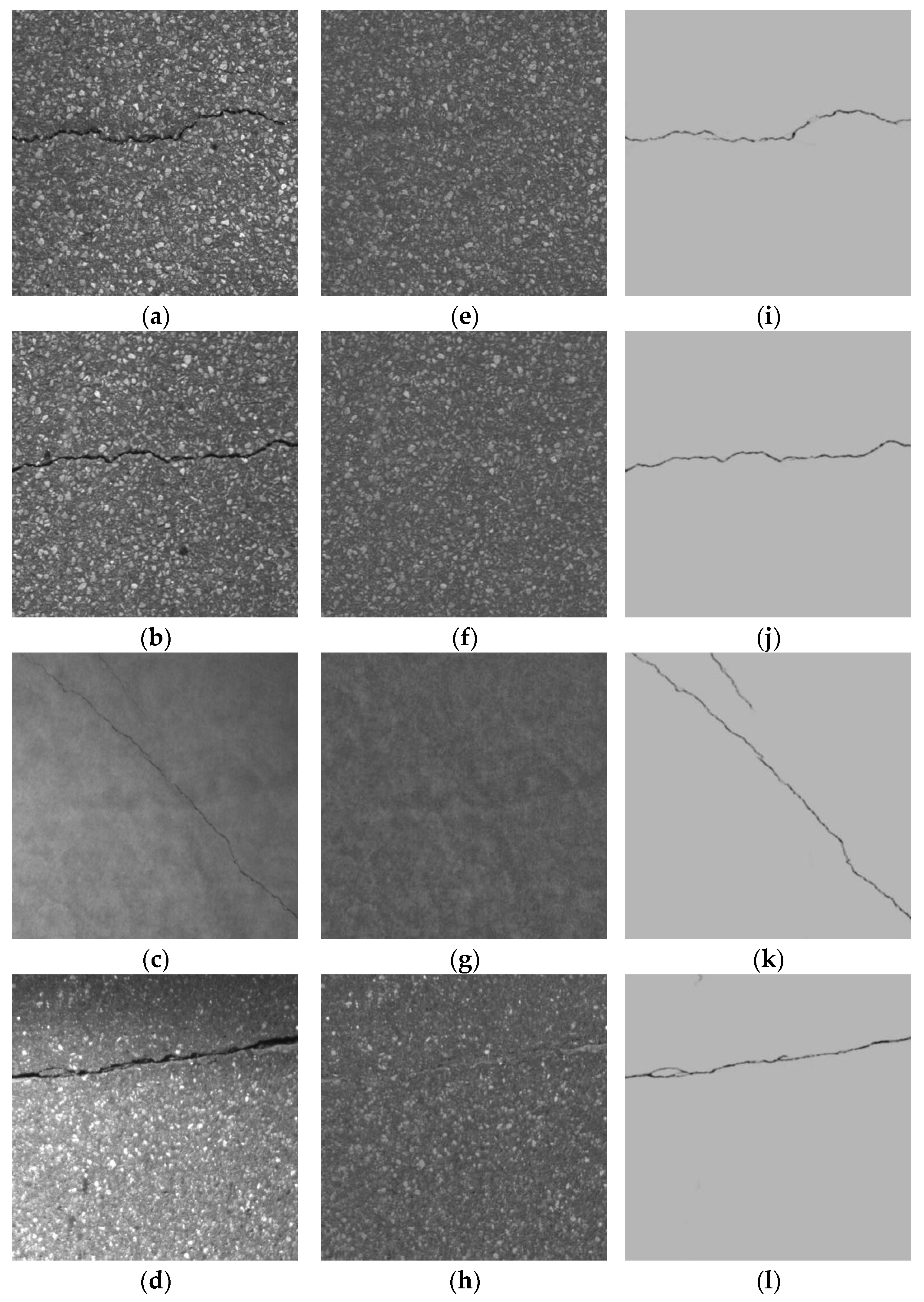
Figure 17a shows the original image, Figure 17b shows its random sampling with gray-scale sparsity prior, and Figure 17c shows pixel label-based crack detection [14], which is the current mainstream method. The pixels (e.g., 5000 pixels) were predicted as a “crack”.

TP is the correctly predicted crack and FP is the incorrectly predicted crack. The accuracy was equal to the percentage of the objects that were correctly predicted as cracks.

Accuracy = TP/S

(26)

The pixel that is falsely predicted as a crack is FP, and the precision is equal to.

Precision = TP/(TP + FP)

(27)

Here, random sampling appears to be an inadequate method due to its low accuracy (about 4.46%) and precision (about 1.35%). Regardless, the semantics of the cracks have preserved. Human vision can easily label the cracks correctly, and our method proves it is also feasibility in computer vision.

Crack detection is a problem characterized by uncertainty and multi-solution. The characteristics of cracks vary, and different individuals may have varying interpretations and ground truths about the same crack. Conventional label based deep learning employs statistics and probability theory to address this uncertainty. The deep learning network counts training samples and determines the consistency between pixels in image and crack semantics-marked pixels. For example, the algorithm assigns a probability value of “it is a crack pixel” to each pixel in the pixel container-based crack detection shown in Figure 17. Thus, an unusual, indistinct, and wide probability line appears when facing uncertain scenarios.

The proposed method initially selects seed pixels randomly as reminders to extract images meeting specified conditions from semantic containers. It then fuses the semantic images and compares them with the original image to correct the incorrect regions. Therefore, the proposed method is essentially a bidirectional heuristic search method utilizing randomly generated seed pixels as hints to find targets that appear simultaneously in image and semantic containers. Comparing the two methods, pixel label-based methods are more likely to perceive any pixels with cracks, while the proposed method appears to be more semantically focused on cognitive cracks.

4. Conclusions

Our initial contribution highlighted that the primary challenge in tunnel image stitching pertained to establishing the relative positional relationship between the camera and the tunnel lining surface. Consequently, the image mapping equations directly obtained via a laser scanner were tantamount to the indirect measurements conducted for the overlapping image regions. For inspection systems that possess both laser scanners and cameras, image-range stitching presents a simpler, more dependable method that deserves further consideration.

Subsequently, we emphasize that pixel-label based crack detection techniques can not actively search for cracks, but rather perceptively any pixels containing cracks. Consequently, we propose a method that is more cognitively focused on semantically identifying cracks. Our work emulates human semantic matching, resulting in a refined algorithmic structure that constitutes a significant advance in the field of artificial intelligence. The development enhances the understanding of cognitive processes. However, mimicking human intelligence does not necessarily imply efficiency, such as the image retrieval process of generating images, which can be rapidly implemented through heuristic image matching algorithms. Meanwhile, limited by the lacking understanding of human cognitive processes, the current method only addresses the issue of crack detection in simplified scenes consisting of cracks and textures. It remains to be seen whether it can tackle more complex scenes, and how to address more complex detection challenges.