
Dynamic Monitoring of Surface Water Bodies and Their Influencing Factors in the Yellow River Basin

Abstract
:1. Introduction
2. Materials and Methods
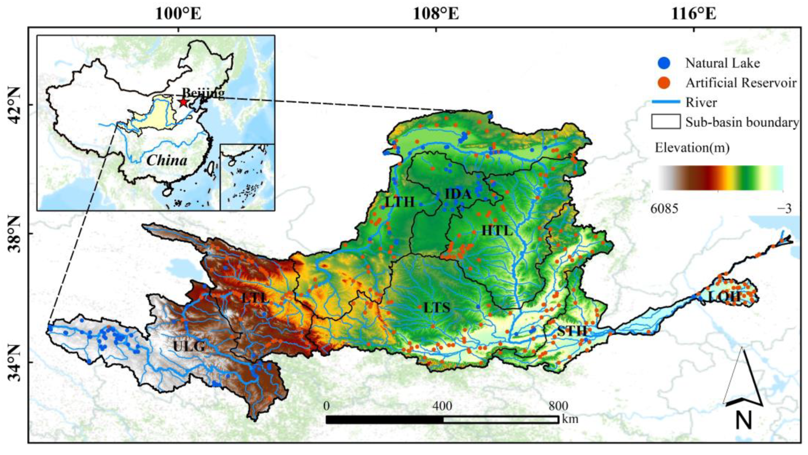
2.1. Study Areas
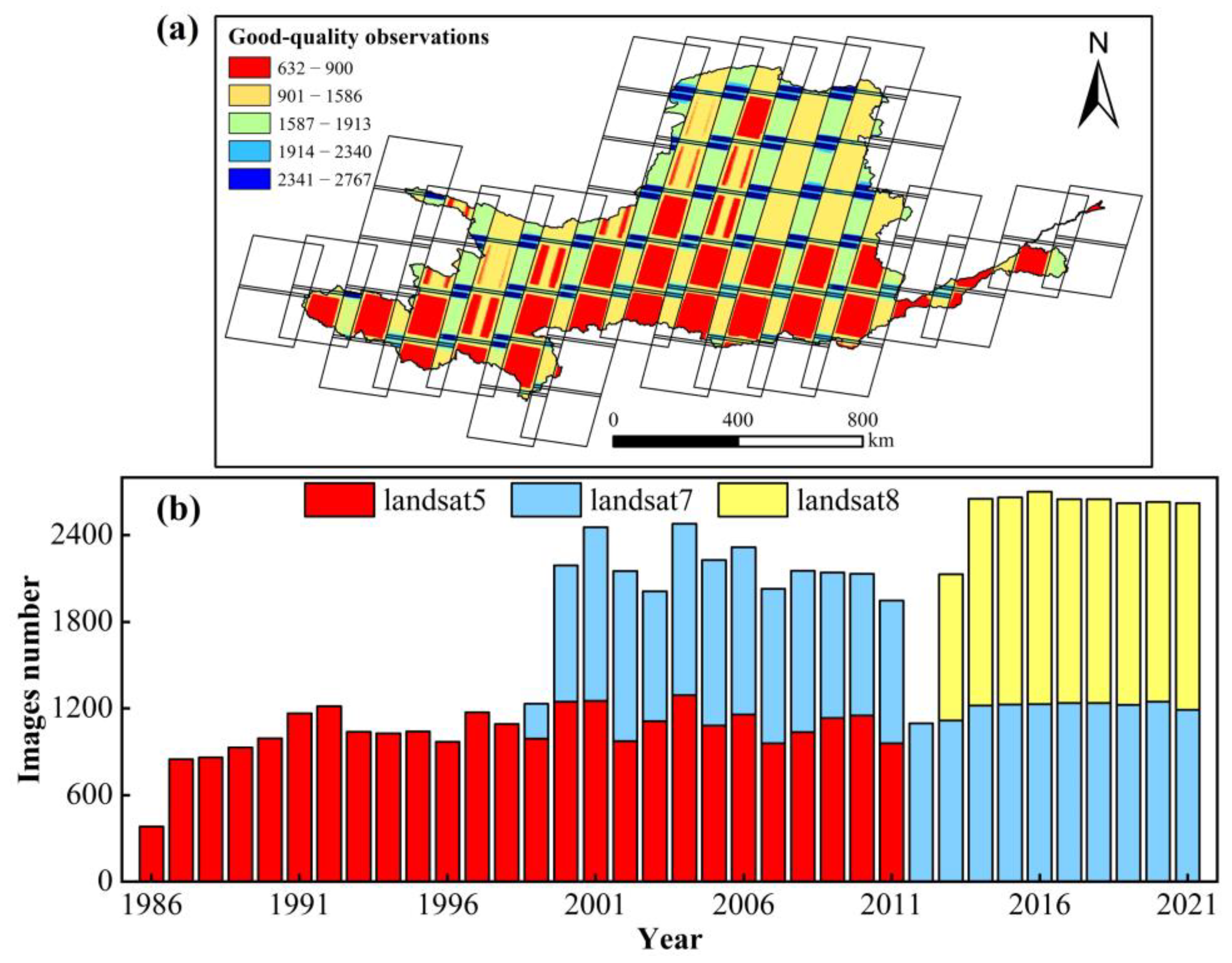
2.2. Data Sources
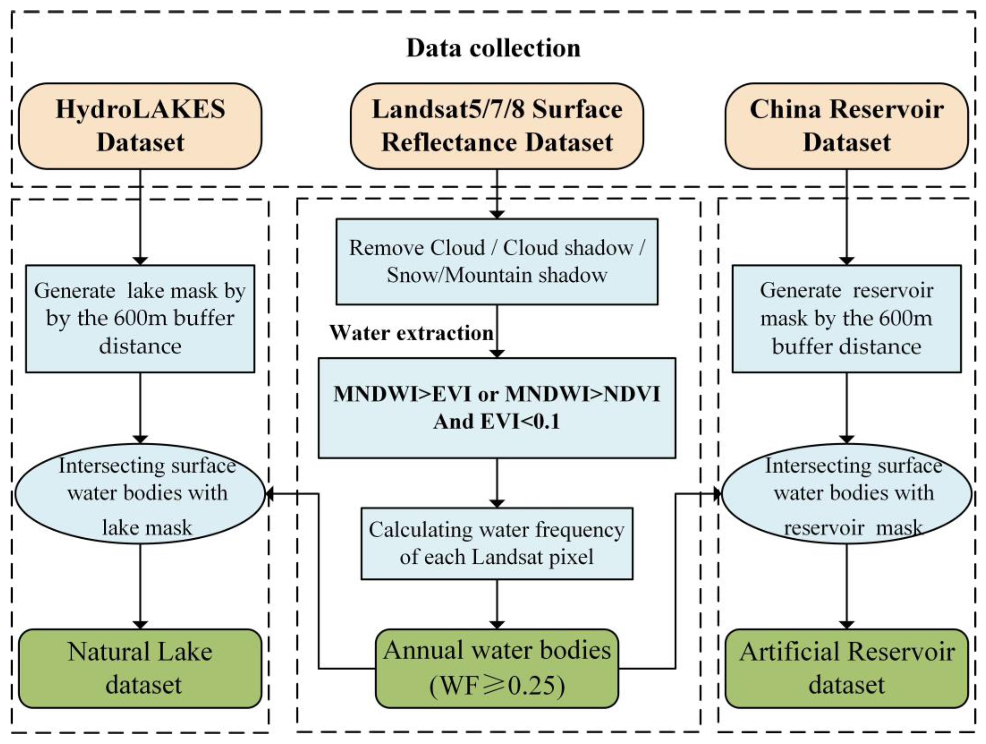
2.3. Methods
2.3.1. Water Extraction Algorithm
2.3.2. Accuracy Assessment
2.3.3. Trend Analysis Methods
2.3.4. Driving Factors of Surface Water Bodies Area Changes
3. Results
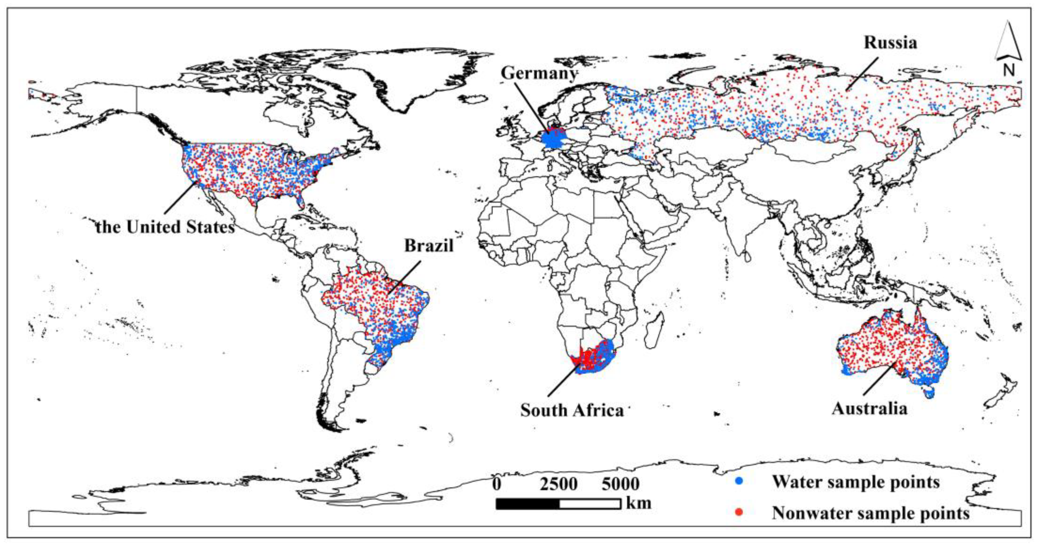
3.1. Accuracy Assessment of Surface Water Bodies
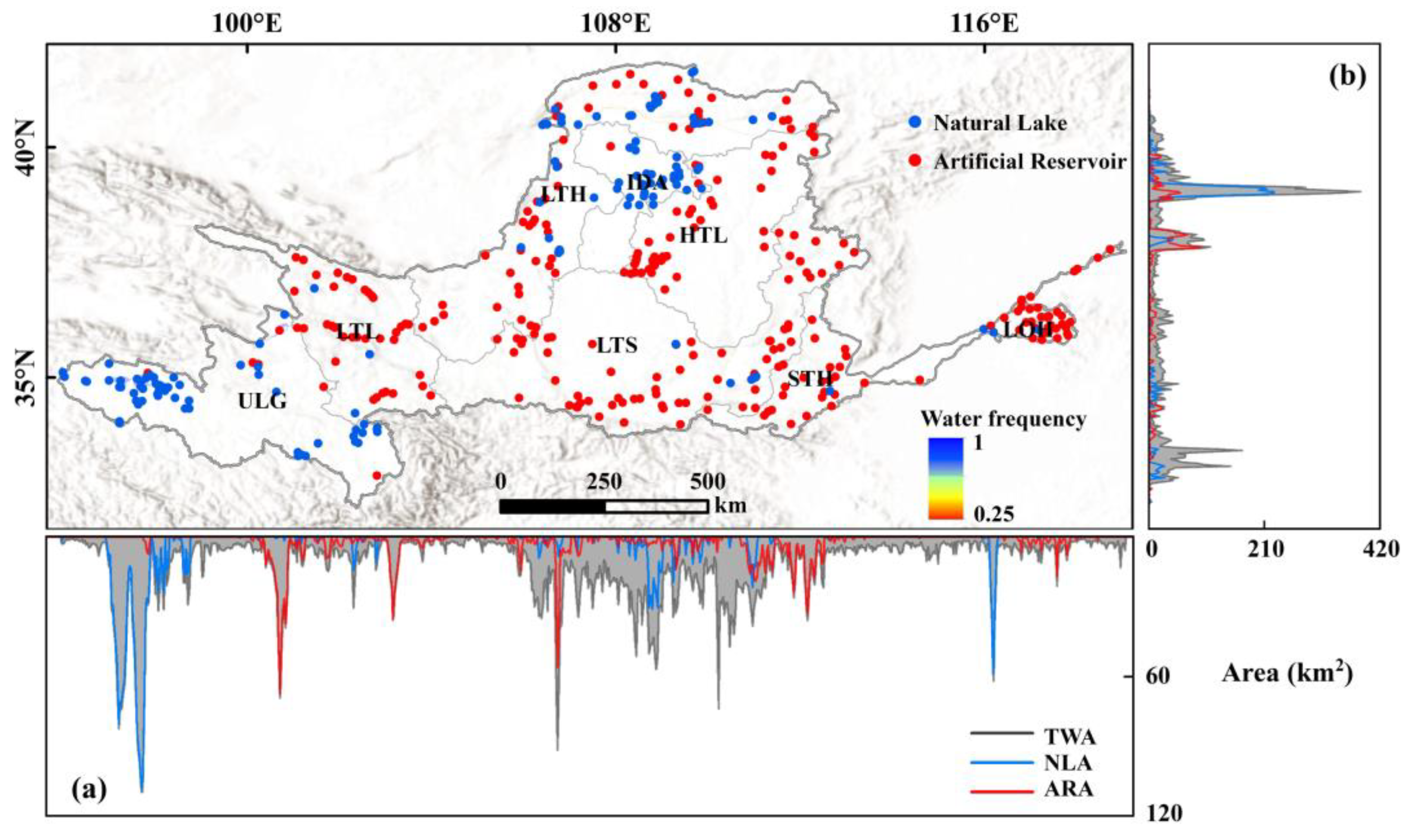
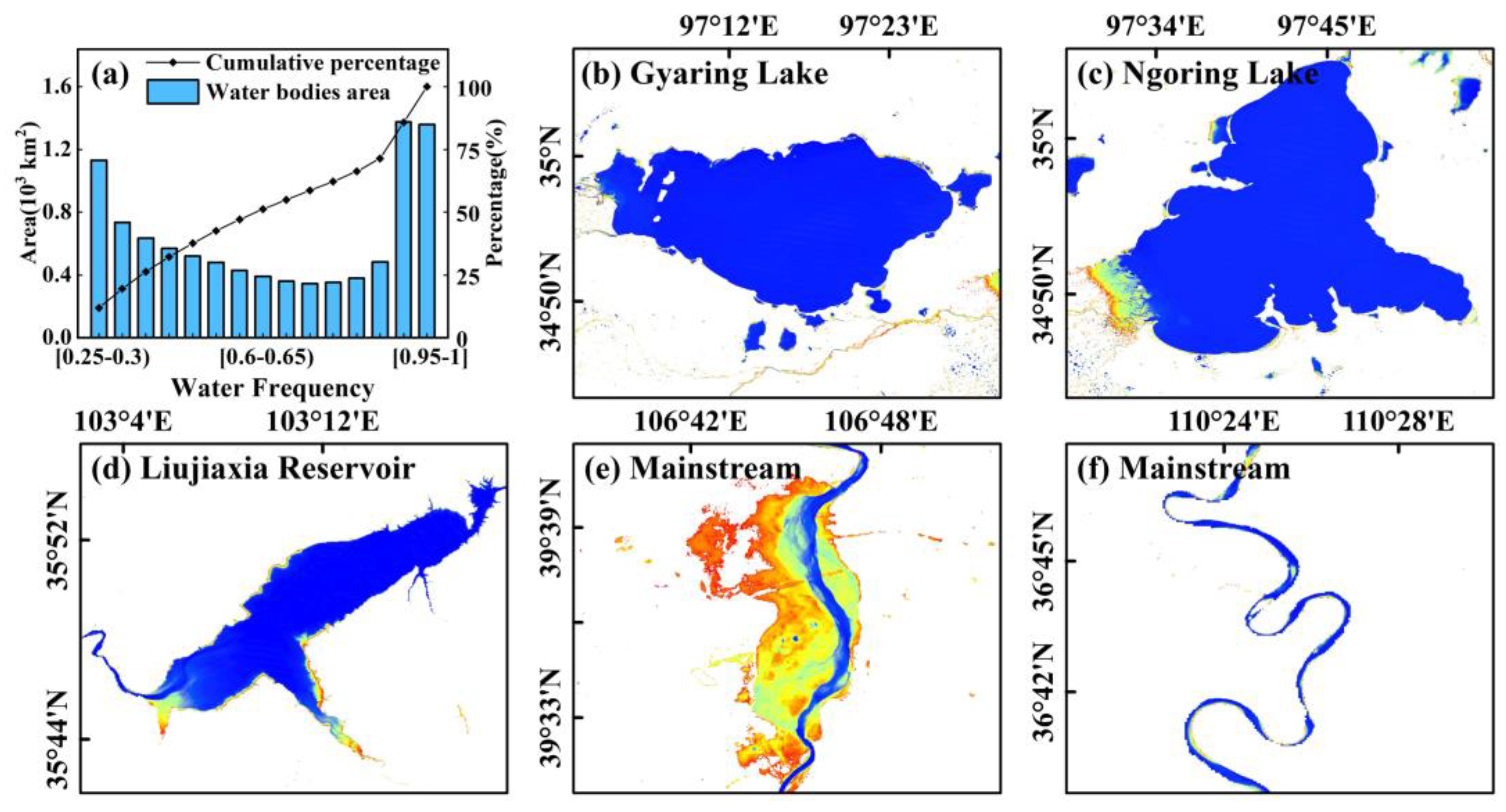
3.2. The Areas of Surface Water Bodies and Spatial Distribution
3.3. Areal Changes of Surface Water Bodies
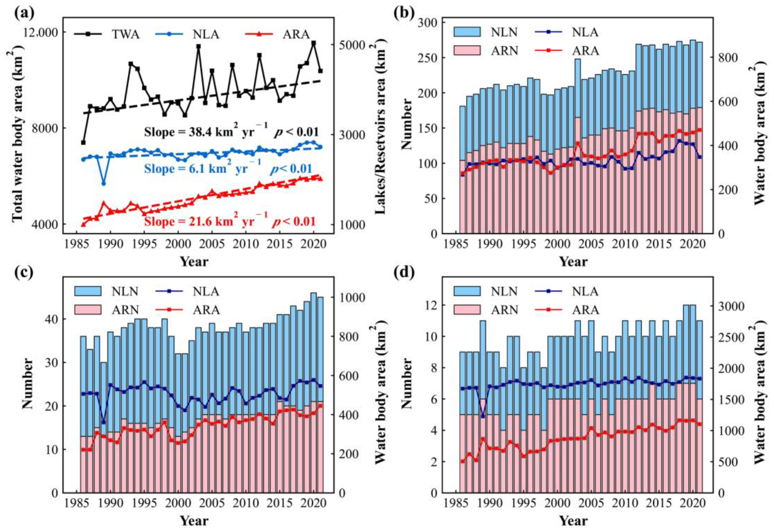
3.3.1. Annual Trends of Surface Water Bodies Area from 1986 to 2021
3.3.2. Spatial Distribution of the Trend of Surface Water Area
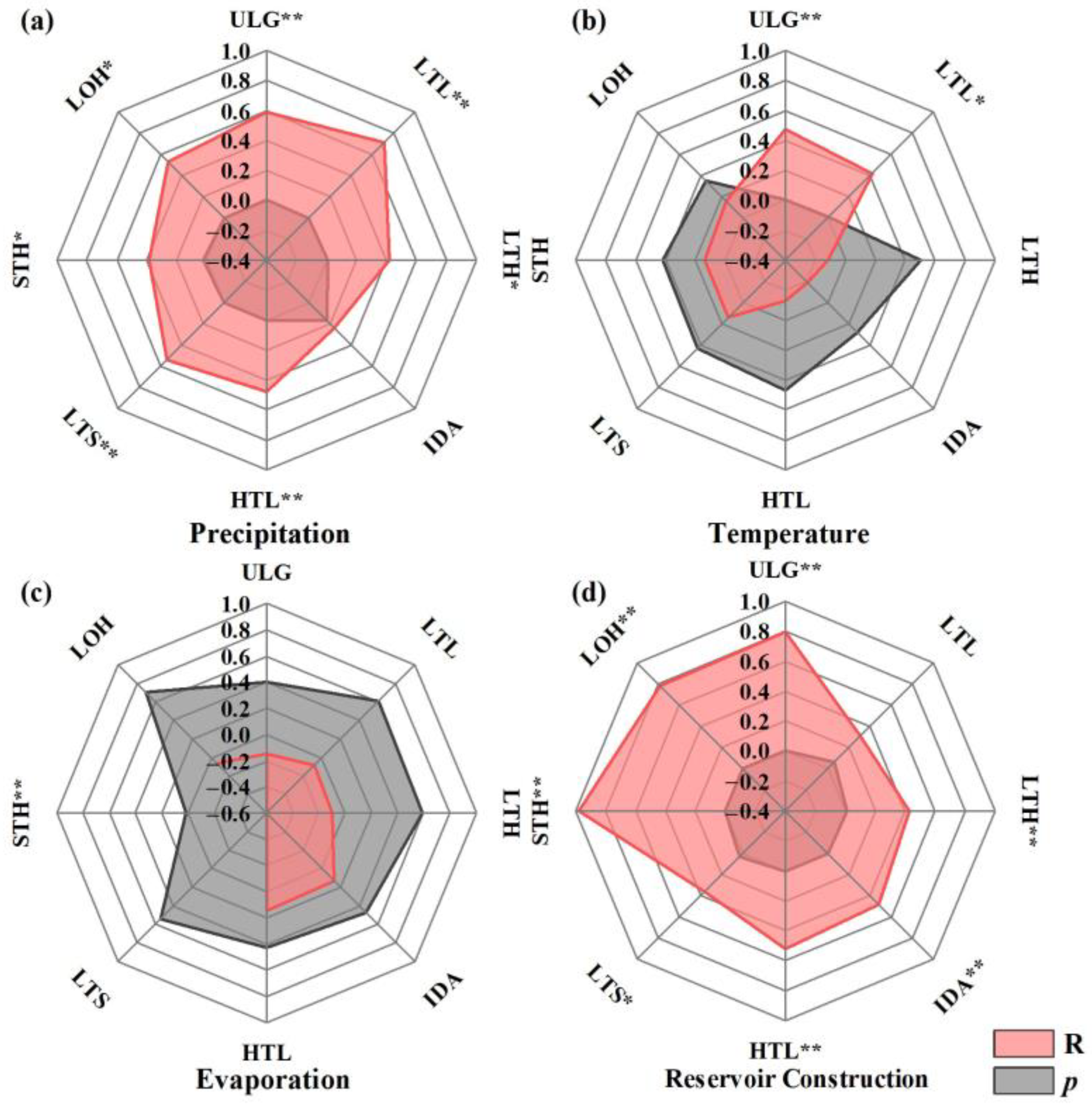
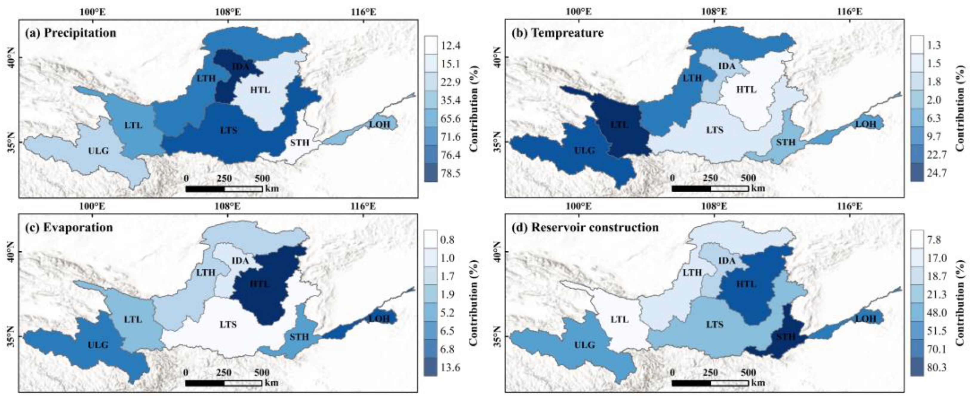
3.4. Drivers of Surface Water Bodies Area Changes
4. Discussion
4.1. Impact of Climate and Human Activities on Changes in Surface Water Bodies
4.2. Performance and Uncertainty of Water Extraction Algorithms
5. Conclusions
Author Contributions
Funding
Data Availability Statement
Conflicts of Interest
References
- McDonald, R.I.; Weber, K.; Padowski, J.; Flörke, M.; Schneider, C.; Green, P.A.; Gleeson, T.; Eckman, S.; Lehner, B.; Balk, D. Water on an urban planet: Urbanization and the reach of urban water infrastructure. Glob. Environ. Chang. 2014, 27, 96–105. [Google Scholar]
- Suring, L.H. Freshwater: Oasis of Life—An Overview. In Encyclopedia of the World’s Biomes; Elsevier: Oxford, UK, 2020; pp. 1–11. [Google Scholar]
- Plessis, A.D. Freshwater and Industries. In Encyclopedia of the World’s Biomes; Elsevier: Oxford, UK, 2020; pp. 55–62. [Google Scholar]
- Edwards, E.C.; Nehra, A. Importance of Freshwater for Irrigation. In Encyclopedia of the World’s Biomes; Elsevier: Oxford, UK, 2020; pp. 22–28. [Google Scholar]
- Ren, L.; Wang, M.; Li, C.; Zhang, W. Impacts of human activity on river runoff in the northern area of China. J. Hydrol. 2002, 261, 204–217. [Google Scholar] [CrossRef]
- Khandelwal, A.; Karpatne, A.; Marlier, M.E.; Kim, J.; Lettenmaier, D.P.; Kumar, V. An approach for global monitoring of surface water extent variations in reservoirs using MODIS data. Remote Sens. Environ. 2017, 202, 113–128. [Google Scholar]
- Klein, I.; Gessner, U.; Dietz, A.J.; Kuenzer, C. Global WaterPack—A 250 m resolution dataset revealing the daily dynamics of global inland water bodies. Remote Sens. Environ. 2017, 198, 345–362. [Google Scholar]
- Berge-Nguyen, M.; Cretaux, J.F. Inundations in the Inner Niger Delta: Monitoring and analysis using MODIS and global precipitation datasets. Remote Sens. 2015, 7, 2127–2151. [Google Scholar]
- Mueller, N.; Lewis, A.; Roberts, D.; Ring, S.; Melrose, R.; Sixsmith, J.; Lymburner, L.; McIntyre, A.; Tan, P.; Curnow, S.; et al. Water observations from space: Mapping surface water from 25 years of Landsat imagery across Australia. Remote Sens. Environ. 2016, 174, 341–352. [Google Scholar] [CrossRef]
- Yao, F.; Wang, J.; Wang, C.; Crétaux, J.-F. Constructing long-term high-frequency time series of global lake and reservoir areas using Landsat imagery. Remote Sens. Environ. 2019, 232, 111210. [Google Scholar] [CrossRef]
- Feyisa, G.L.; Meilby, H.; Fensholt, R.; Proud, S.R. Automated Water Extraction Index: A new technique for surface water mapping using Landsat imagery. Remote Sens. Environ. 2014, 140, 23–35. [Google Scholar] [CrossRef]
- Yamazaki, D.; Trigg, M.A.; Ikeshima, D. Development of a global similar to 90 m water body map using multi-temporal Landsat images. Remote Sens. Environ. 2015, 171, 337–351. [Google Scholar] [CrossRef]
- Schwatke, C.; Scherer, D.; Dettmering, D. Automated Extraction of Consistent Time-Variable Water Surfaces of Lakes and Reservoirs Based on Landsat and Sentinel-2. Remote Sens. 2019, 11, 1010. [Google Scholar]
- Steinhausen, M.J.; Wagner, P.D.; Narasimhan, B.; Waske, B. Combining Sentinel-1 and Sentinel-2 data for improved land use and land cover mapping of monsoon regions. Int. J. Appl. Earth Obs. Geoinf. 2018, 73, 595–604. [Google Scholar]
- Jakovljevic, G.; Govedarica, M.; Alvarez-Taboada, F. Waterbody mapping: A comparison of remotely sensed and GIS open data sources. Int. J. Remote Sens. 2019, 40, 2936–2964. [Google Scholar]
- Gómez, C.; White, J.C.; Wulder, M.A. Optical remotely sensed time series data for land cover classification: A review. ISPRS J. Photogramm. Remote Sens. 2016, 116, 55–72. [Google Scholar] [CrossRef]
- Wang, Y.; Ma, J.; Xiao, X.; Wang, X.; Zhao, B. Long-Term Dynamic of Poyang Lake Surface Water: A Mapping Work Based on the Google Earth Engine Cloud Platform. Remote Sens. 2019, 11, 313. [Google Scholar] [CrossRef]
- Halabisky, M.; Moskal, L.M.; Gillespie, A.; Hannam, M. Reconstructing semi-arid wetland surface water dynamics through spectral mixture analysis of a time series of Landsat satellite images (1984–2011). Remote Sens. Environ. 2016, 177, 171–183. [Google Scholar] [CrossRef]
- Tedros, B.; Charles, L.; Wu, Q.; Bradley, A.; Oleg, A.; Victor, C.; Liu, H. Decision-Tree, Rule-Based, and Random Forest Classification of High-Resolution Multispectral Imagery for Wetland Mapping and Inventory. Remote Sens. 2018, 10, 580. [Google Scholar]
- McFeeters, S.K. The use of the Normalized Difference Water Index (NDWI) in the delineation of open water features. Int. J. Remote Sens. 1996, 17, 1425–1432. [Google Scholar]
- Xu, H. Modification of normalised difference water index (NDWI) to enhance open water features in remotely sensed imagery. Int. J. Remote Sens. 2006, 27, 3025–3033. [Google Scholar]
- Tulbure, M.G.; Broich, M.; Stehman, S.V.; Kommareddy, A. Surface water extent dynamics from three decades of seasonally continuous Landsat time series at subcontinental scale in a semi-arid region. Remote Sens. Environ. 2016, 178, 142–157. [Google Scholar]
- Otsu, N. A Threshold Selection Method from Gray-Level Histograms. IEEE Trans. Syst. Man Cybern. 2007, 9, 62–66. [Google Scholar] [CrossRef]
- Yang, X.; Qin, Q.; Grussenmeyer, P.; Koehl, M. Urban surface water body detection with suppressed built-up noise based on water indices from Sentinel-2 MSI imagery. Remote Sens. Environ. 2018, 219, 259–270. [Google Scholar] [CrossRef]
- Han, Q.; Niu, Z. Construction of the Long-Term Global Surface Water Extent Dataset Based on Water-NDVI Spatio-Temporal Parameter Sets. Remote Sens. 2020, 12, 2675. [Google Scholar] [CrossRef]
- Gorelick, N.; Hancher, M.; Dixon, M.; Ilyushchenko, S.; Thau, D.; Moore, R. Google Earth Engine: Planetary-scale geospatial analysis for everyone. Remote Sens. Environ. 2017, 202, 18–27. [Google Scholar] [CrossRef]
- Zurqani, H.A.; Post, C.J.; Mikhailova, E.A.; Schlautman, M.A.; Sharp, J.L. Geospatial analysis of land use change in the Savannah River Basin using Google Earth Engine. Int. J. Appl. Earth Obs. Geoinf. 2018, 69, 175–185. [Google Scholar] [CrossRef]
- Chen, B.; Xiao, X.; Li, X.; Pan, L.; Doughty, R.; Ma, J.; Dong, J.; Qin, Y.; Zhao, B.; Wu, Z. A mangrove forest map of China in 2015: Analysis of time series Landsat 7/8 and Sentinel-1A imagery in Google Earth Engine cloud computing platform. ISPRS J. Photogramm. Remote Sens. 2017, 131, 104–120. [Google Scholar] [CrossRef]
- Liu, X.; Hu, G.; Chen, Y.; Xia, L.; Pei, F. High-resolution multi-temporal mapping of global urban land using Landsat images based on the Google Earth Engine Platform. Remote Sens. Environ. 2018, 209, 227–239. [Google Scholar] [CrossRef]
- Murray, N.J.; Phinn, S.R.; DeWitt, M.; Ferrari, R.; Johnston, R.; Lyons, M.B.; Clinton, N.; Thau, D.; Fuller, R.A. The global distribution and trajectory of tidal flats. Nature 2019, 565, 222–225. [Google Scholar] [CrossRef] [PubMed]
- Pekel, J.F.; Cottam, A.; Gorelick, N.; Belward, A.S. High-resolution mapping of global surface water and its long-term changes. Nature 2016, 540, 418–422. [Google Scholar] [CrossRef] [PubMed]
- Zou, Z.; Xiao, X.; Dong, J.; Qin, Y.; Doughty, R.B.; Menarguez, M.A.; Zhang, G.; Wang, J. Divergent trends of open-surface water body area in the contiguous United States from 1984 to 2016. Proc. Natl. Acad. Sci. USA 2018, 115, 3810–3815. [Google Scholar] [CrossRef]
- Wang, X.; Xiao, X.; Zou, Z.; Dong, J.; Qin, Y.; Doughty, R.B.; Menarguez, M.A.; Chen, B.; Wang, J.; Ye, H.; et al. Gainers and losers of surface and terrestrial water resources in China during 1989–2016. Nat. Commun. 2020, 11, 3471. [Google Scholar] [CrossRef]
- Xie, J.; Xu, Y.-P.; Wang, Y.; Gu, H.; Wang, F.; Pan, S. Influences of climatic variability and human activities on terrestrial water storage variations across the Yellow River basin in the recent decade. J. Hydrol. 2019, 579, 124218. [Google Scholar] [CrossRef]
- Liu, Y.; Song, H.; An, Z.; Sun, C.; Trouet, V.; Cai, Q.; Liu, R.; Leavitt, S.W.; Song, Y.; Li, Q.; et al. Recent anthropogenic curtailing of Yellow River runoff and sediment load is unprecedented over the past 500 y. Proc. Natl. Acad. Sci. USA 2020, 117, 18251–18257. [Google Scholar] [CrossRef] [PubMed]
- Șerban, R.D.; Jin, H.; Șerban, M.; Luo, D. Shrinking thermokarst lakes and ponds on the northeastern Qinghai-Tibet plateau over the past three decades. Permafr. Periglac. Process. 2021, 32, 601–617. [Google Scholar] [CrossRef]
- Zhou, H.; Liu, S.; Hu, S.; Mo, X. Retrieving dynamics of the surface water extent in the upper reach of Yellow River. Sci. Total Environ. 2021, 800, 149348. [Google Scholar] [CrossRef]
- Wang, R.; Xia, H.; Qin, Y.; Niu, W.; Pan, L.; Li, R.; Zhao, X.; Bian, X.; Fu, P. Dynamic Monitoring of Surface Water Area during 1989–2019 in the Hetao Plain Using Landsat Data in Google Earth Engine. Water 2020, 12, 3010. [Google Scholar] [CrossRef]
- Yan, D.; Wang, X.; Zhu, X.; Huang, C.; Li, W. Analysis of the use of NDWIgreen and NDWIred for inland water mapping in the Yellow River Basin using Landsat-8 OLI imagery. Remote Sens. Lett. 2017, 8, 996–1005. [Google Scholar] [CrossRef]
- Yang, D.; Li, C.; Hu, H.; Lei, Z.; Yang, S.; Kusuda, T.; Koike, T.; Musiake, K. Analysis of water resources variability in the Yellow River of China during the last half century using historical data. Water Resour. Res. 2004, 40, W06502. [Google Scholar] [CrossRef]
- Wang, W.; Shao, Q.; Peng, S.; Xing, W.; Yang, T.; Luo, Y.; Yong, B.; Xu, J. Reference evapotranspiration change and the causes across the Yellow River Basin during 1957–2008 and their spatial and seasonal differences. Water Resour. Res. 2012, 48, W05530. [Google Scholar] [CrossRef]
- Song, C.; Fan, C.; Zhu, J.; Wang, J.; Sheng, Y.; Liu, K.; Chen, T.; Zhan, P.; Luo, S.; Yuan, C. A comprehensive geospatial database of nearly 100,000 reservoirs in China. Earth Syst. Sci. Data 2022, 14, 4017–4034. [Google Scholar] [CrossRef]
- Xia, H.; Zhao, J.; Qin, Y.; Yang, J.; Cui, Y.; Song, H.; Ma, L.; Jin, N.; Meng, Q. Changes in Water Surface Area during 1989–2017 in the Huai River Basin using Landsat Data and Google Earth Engine. Remote Sens. 2019, 11, 1824. [Google Scholar] [CrossRef]
- Huang, J.; Zhang, G.; Zhang, Y.; Guan, X.; Wei, Y.; Guo, R. Global desertification vulnerability to climate change and human activities. Land Degrad. Dev. 2020, 31, 1380–1391. [Google Scholar]
- Li, Z.; Yan, Z.; Zhu, Y.; Freychet, N.; Tett, S. Homogenized daily relative humidity series in China during 1960–2017. Adv. Atmos. Sci. 2020, 37, 318–327. [Google Scholar]
- Wang, X.; Xiao, X.; Zou, Z.; Chen, B.; Ma, J.; Dong, J.; Doughty, R.B.; Zhong, Q.; Qin, Y.; Dai, S.; et al. Tracking annual changes of coastal tidal flats in China during 1986–2016 through analyses of Landsat images with Google Earth Engine. Remote Sens. Environ. 2020, 238, 110987. [Google Scholar] [CrossRef] [PubMed]
- Santoro, M.; Wegmuller, U.; Lamarche, C.; Bontemps, S.; Defoumy, P.; Arino, O. Strengths and weaknesses of multi-year Envisat ASAR backscatter measurements to map permanent open water bodies at global scale. Remote Sens. Environ. 2015, 171, 185–201. [Google Scholar] [CrossRef]
- Dong, J.W.; Xiao, X.M.; Kou, W.L.; Qin, Y.W.; Zhang, G.L.; Li, L.; Jin, C.; Zhou, Y.T.; Wang, J.; Biradar, C.; et al. Tracking the dynamics of paddy rice planting area in 1986–2010 through time series Landsat images and phenology-based algorithms. Remote Sens. Environ. 2015, 160, 99–113. [Google Scholar] [CrossRef]
- Zou, Z.; Dong, J.; Menarguez, M.A.; Xiao, X.; Qin, Y.; Doughty, R.B.; Hooker, K.V.; David Hambright, K. Continued decrease of open surface water body area in Oklahoma during 1984–2015. Sci. Total Environ. 2017, 595, 451–460. [Google Scholar] [CrossRef]
- Zhao, G.; Li, Y.; Zhou, L.; Gao, H. Evaporative water loss of 1.42 million global lakes. Nat. Commun. 2022, 13, 3686. [Google Scholar] [PubMed]
- Sen, K.P. Estimates of the Regression Coefficient Based on Kendall’s Tau. Publ. Am. Stat. Assoc. 1968, 63, 1379–1389. [Google Scholar] [CrossRef]
- Mann, H.B. Nonparametric test against trend. Econometrica 1945, 13, 245–259. [Google Scholar] [CrossRef]
- Kendall, S.B. Enhancement of conditioned reinforcement by uncertainty. J. Exp. Anal. Behav. 1975, 24, 311–314. [Google Scholar]
- Woolway, R.I.; Kraemer, B.M.; Lenters, J.D.; Merchant, C.J.; O’Reilly, C.M.; Sharma, S. Global lake responses to climate change. Nat. Rev. Earth Environ. 2020, 1, 388–403. [Google Scholar]
- Shugar, D.H.; Burr, A.; Haritashya, U.K.; Kargel, J.S.; Watson, C.S.; Kennedy, M.C.; Bevington, A.R.; Betts, R.A.; Harrison, S.; Strattman, K. Rapid worldwide growth of glacial lakes since 1990. Nat. Clim. Change 2020, 10, 939–945. [Google Scholar] [CrossRef]
- van Dijk, A.; Beck, H.E.; Crosbie, R.S.; de Jeu, R.A.M.; Liu, Y.Y.; Podger, G.M.; Timbal, B.; Viney, N.R. The Millennium Drought in southeast Australia (2001–2009): Natural and human causes and implications for water resources, ecosystems, economy, and society. Water Resour. Res. 2013, 49, 1040–1057. [Google Scholar] [CrossRef]
- Pi, X.; Luo, Q.; Feng, L.; Xu, Y.; Tang, J.; Liang, X.; Ma, E.; Cheng, R.; Fensholt, R.; Brandt, M.; et al. Mapping global lake dynamics reveals the emerging roles of small lakes. Nat. Commun. 2022, 13, 5777. [Google Scholar] [CrossRef] [PubMed]
- Zhu, Y.; Ye, A.; Zhang, Y. Changes of total and artificial water bodies in inland China over the past three decades. J. Hydrol. 2022, 613, 128344. [Google Scholar]
- Liu, Y.; Wu, G.; Zhao, X. Recent declines in China’s largest freshwater lake: Trend or regime shift? Environ. Res. Lett. 2013, 8, 014010. [Google Scholar] [CrossRef]
- Deng, Y.; Jiang, W.; Tang, Z.; Ling, Z.; Wu, Z. Long-term changes of open-surface water bodies in the Yangtze River basin based on the Google Earth Engine cloud platform. Remote Sens. 2019, 11, 2213. [Google Scholar]
- Luo, D.; Jin, H.; Du, H.; Li, C.; Ma, Q.; Duan, S.; Li, G. Variation of alpine lakes from 1986 to 2019 in the Headwater Area of the Yellow River, Tibetan Plateau using Google Earth Engine. Adv. Clim. Chang. Res. 2020, 11, 11–21. [Google Scholar] [CrossRef]
- Wang, D.; Alimohammadi, N. Responses of annual runoff, evaporation, and storage change to climate variability at the watershed scale. Water Resour. Res. 2012, 48, W05546. [Google Scholar]
- Vorosmarty, C.J.; Green, P.; Salisbury, J.; Lammers, R.B. Global Water Resources: Vulnerability from Climate Change and Population Growth. Science 2000, 289, 284–288. [Google Scholar]
- Biemans, H.; Haddeland, I.; Kabat, P.; Ludwig, F.; Hutjes, R.W.A.; Heinke, J.; von Bloh, W.; Gerten, D. Impact of reservoirs on river discharge and irrigation water supply during the 20th century. Water Resour. Res. 2011, 47, W03509. [Google Scholar] [CrossRef]
- Zhou, Y.; Dong, J.; Xiao, X.; Xiao, T.; Yang, Z.; Zhao, G.; Zou, Z.; Qin, Y. Open surface water mapping algorithms: A comparison of water-related spectral indices and sensors. Water 2017, 9, 256. [Google Scholar]
- Wang, X.; Wang, W.; Jiang, W.; Jia, K.; Rao, P.; Lv, J. Analysis of the Dynamic Changes of the Baiyangdian Lake Surface Based on a Complex Water Extraction Method. Water 2018, 10, 1616. [Google Scholar] [CrossRef]
- Fisher, A.; Flood, N.; Danaher, T. Comparing Landsat water index methods for automated water classification in eastern Australia. Remote Sens. Environ. 2016, 175, 167–182. [Google Scholar] [CrossRef]


| Sample Number | Sample Number | Total | UA | |
|---|---|---|---|---|
| Water | Non-Water | |||
| Water | 4235 | 70 | 4305 | 98.37% |
| Non-Water | 106 | 3589 | 3695 | 97.13% |
| Total | 4573 | 3659 | OA = 97.80% | |
| PA | 97.56% | 98.09% | Kc = 0.96 | |
| TWA (km2) | NLA (km2)/ Proportion of TWA (%) | ARA (km2)/ Proportion of TWA (%) | |
|---|---|---|---|
| YRB | 9549.5 | 2528.0/26.5 | 1871.7/19.6 |
| ULG | 2963.6 | 1772.3/59.8 | 444.9/15.0 |
| LTL | 531.9 | 21.1/4.0 | 310.9/58.5 |
| IDA | 408.4 | 187.9/46.0 | 16.5/4.0 |
| LTH | 2824.0 | 303.1/10.7 | 288.1/10.2 |
| HTL | 498.5 | 13.5/2.7 | 129.5/26.0 |
| LTS | 893.6 | 64.0/7.2 | 314.4/35.2 |
| STH | 495.1 | 3.4/0.7 | 274.2/55.4 |
| LOH | 934.4 | 162.7/17.4 | 93.2/10.0 |
| Precipitation (mm yr−1) | Temperature (°C yr−1) | Evaporation (mm yr−1) | |
|---|---|---|---|
| YRB | 3.85 ** | 0.04 ** | −0.35 |
| ULG | 5.97 ** | 0.03 ** | 0.40 * |
| LTL | 3.75 ** | 0.04 ** | 0.31 * |
| IDA | 2.41 ** | 0.03 ** | −1.41 |
| LTH | 2.48 * | 0.03 ** | −1.33 |
| HTL | 4.44 ** | 0.04 ** | −0.78 |
| LTS | 4.46 ** | 0.03 ** | −0.16 |
| STH | 4.01 * | 0.04 ** | −0.15 |
| LOH | 3.50 | 0.03 ** | −0.23 |
| Regions | OA | Kc |
|---|---|---|
| The United State | 97.12% | 0.94 |
| Brazil | 96.25% | 0.93 |
| Germany | 97.80% | 0.96 |
| South Africa | 96.57% | 0.93 |
| Russia | 96.11% | 0.93 |
| Australia | 97.01% | 0.94 |
| The Yellow River Basin | 97.80% | 0.96 |
Disclaimer/Publisher’s Note: The statements, opinions and data contained in all publications are solely those of the individual author(s) and contributor(s) and not of MDPI and/or the editor(s). MDPI and/or the editor(s) disclaim responsibility for any injury to people or property resulting from any ideas, methods, instructions or products referred to in the content. |
© 2023 by the authors. Licensee MDPI, Basel, Switzerland. This article is an open access article distributed under the terms and conditions of the Creative Commons Attribution (CC BY) license (https://creativecommons.org/licenses/by/4.0/).
Share and Cite
Zhao, Z.; Li, H.; Song, X.; Sun, W. Dynamic Monitoring of Surface Water Bodies and Their Influencing Factors in the Yellow River Basin. Remote Sens. 2023, 15, 5157. https://doi.org/10.3390/rs15215157
Zhao Z, Li H, Song X, Sun W. Dynamic Monitoring of Surface Water Bodies and Their Influencing Factors in the Yellow River Basin. Remote Sensing. 2023; 15(21):5157. https://doi.org/10.3390/rs15215157
Chicago/Turabian StyleZhao, Zikun, Huanwei Li, Xiaoyan Song, and Wenyi Sun. 2023. "Dynamic Monitoring of Surface Water Bodies and Their Influencing Factors in the Yellow River Basin" Remote Sensing 15, no. 21: 5157. https://doi.org/10.3390/rs15215157
APA StyleZhao, Z., Li, H., Song, X., & Sun, W. (2023). Dynamic Monitoring of Surface Water Bodies and Their Influencing Factors in the Yellow River Basin. Remote Sensing, 15(21), 5157. https://doi.org/10.3390/rs15215157